
From Traditional to Electrified Urban Road Networks: The Integration of Fuzzy Analytic Hierarchy Process and GIS as a Tool to Define a Feasibility Index—An Italian Case Study


Abstract
:1. Introduction
2. Literature Review and Objectives
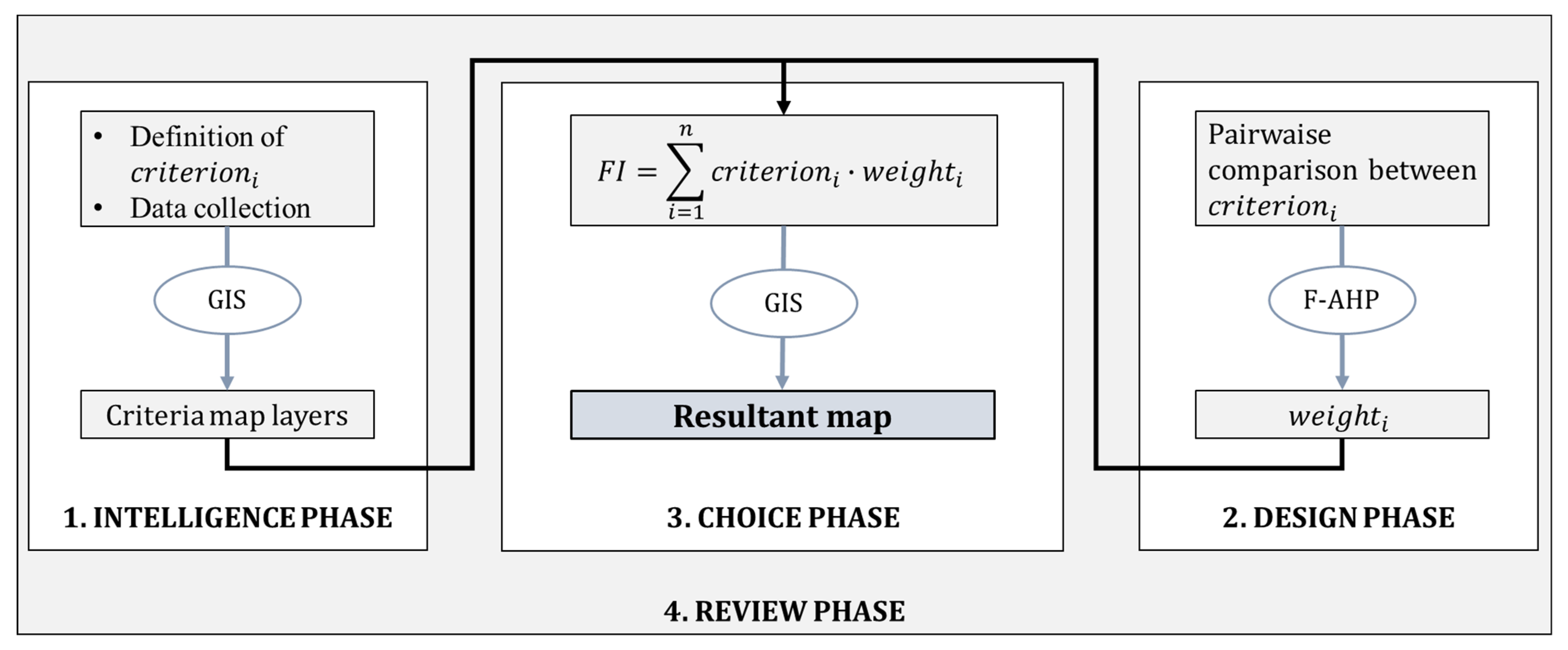
- Intelligence: the problem is structured and the related descriptive criteria are defined. Data of each criterion are collected and processed;
- Design: development of the multicriteria structure, in which the relationships between criteria are described: both normalization and weighting process are performed; regarding the latter, the collection of public/general opinion regarding the main defined problem is currently based on surveys;
- Choice: the different alternatives are compared and assessed for achieving the right solution, answering the question posed by the main problem;
- Review: due to the subjectivity of some steps above described, a sensitivity analysis is performed to increase the decision model reliability and robustness.
3. Intelligence Phase: Criteria Definition, Data Collection and Processing
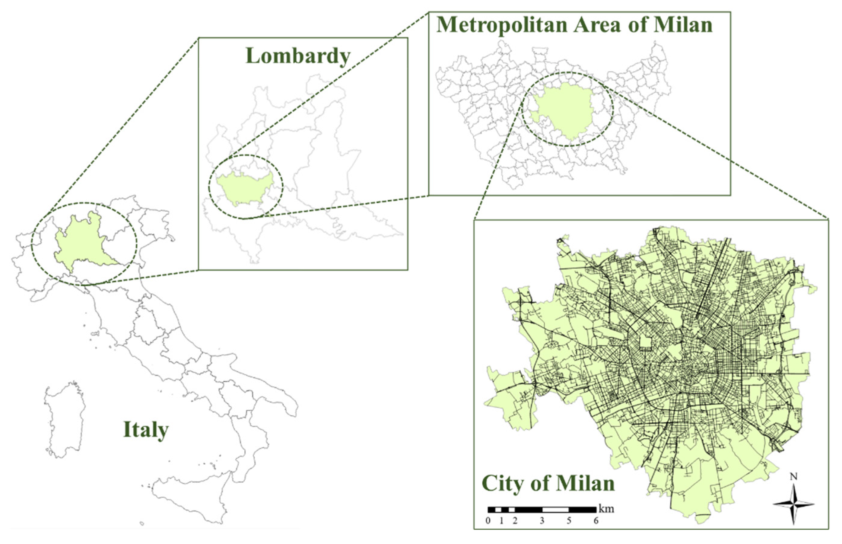
- From a theoretical point of view, the analysis must consider data in a wider area than that considered as a case study (the city of Milan), according to [4]. However, data related to the surrounding areas close to Milan suffer from a lack of information and are not as precise as those from Milan. Therefore, the data considered in the case study are from the city of Milan, except for “Air Quality”, as discussed in the following;
- The year of analysis is 2019, since 2020 data (even when accessible) were affected by the COVID-19 pandemic.
- Road Characteristics (RC): this criterion describes Italian road categories according to [19]: A (extra-urban and urban), B (extra-urban), D (urban) two carriageways and four lanes; E (urban), C (extra-urban) single carriageway and two lanes; F (urban and extra-urban) local/rural roads. The values were set to promote urban environment and lower travel speeds, with the goal of maximizing the vehicle-charging efficiency [5,10,20].
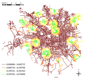
- Vehicle Density (VD): this parameter examines the vehicles (number of vehicles per km2) within the city of Milan. Information about vehicle distribution within the city is difficult to find, because of privacy issues. Therefore, vehicle density was correlated to the population density (PD) of each Milan neighborhood [21], as shown in Equation (1). This assumption implies that the greatest number of vehicles occurs where the greatest number of people live. Since EV number is limited compared with the total vehicle fleet (in Italy, during 2019, EV accounted for 0.057% of the total [22]), VD considers all vehicles without making a distinction between EV and vehicles with other power supplies.By extension, roads acquire the vehicle density value of the neighborhood (VDneighborhood) in which they are located. Once the vehicle density was computed, four intervals were defined to which to assign parameter values, as shown in Table 2 (intelligence phase column). These VD intervals were obtained using the Jenks natural breaks method [23,24]. The values were set to promote high density urban areas, assuming that a high density entailed a higher number of e-road users. Moreover, since each GIS road is made of various lines, it is possible to have a road characterized by various parameter values (VDi). Therefore, in order to obtain one value for each road (VDroad), a length weighted mean is applied, as shown in Equation (2).
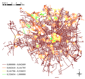
- Traffic (T): this criterion considers the Annual Average Daily Traffic (AADT) traveling on each road. Although the ideal scenario would directly correlate the observed traffic with the road, it was not possible to create an intersection between the network containing the traffic data (traffic data map) and the road network of the city of Milan, due to technical issues. Therefore, an approximation was made by correlating the traffic to both road category (according to [19]) and neighborhood.By intersecting the traffic data map and the neighborhood map, an average value for AADT was calculated according to road category and neighborhood, then it was located into the road network map according to road category and neighborhood. Thus, four intervals were defined to which to assign parameter values, as shown in Table 2 (intelligence phase column). Also in this case, T intervals were outlined using the Jenks natural breaks method. Moreover, in line with the previous parameter, the value for each road (Troad) was calculated by adapting Equation (2).
- Key Infrastructures (KI): this parameter includes point- infrastructures of strategic interest for the city of Milan, whose importance attracts high levels of traffic. In this context, KI are Park-and-Ride facilities [25] and the city airport (Linate) [26]. The parameter values were defined as follows:
- based on the distance as the crow flies from the center of the strategic infrastructure (the shorter the distance, the greater the value);
- based on the strategic infrastructure density (the greater the number of strategic infrastructures, the greater the value).
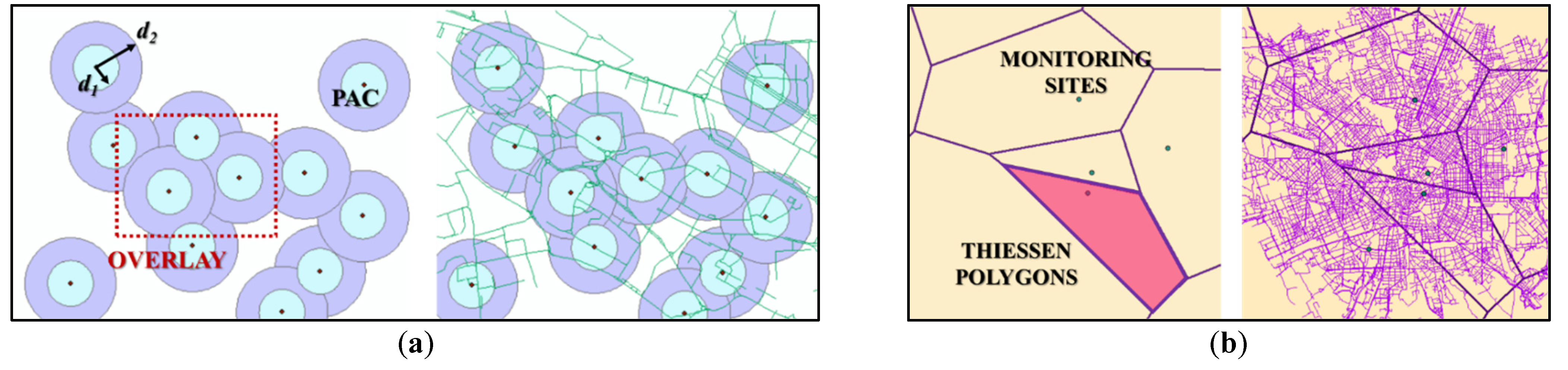
The adopted data processing methodology is known as “multiple/multi ring buffer” (GIS software).By extension, roads acquire the parameter value according to their position in the “multiple ring buffer” geometry. An example of the methodology is shown in Figure 5a.Moreover, in line with the previous parameters, the value for each road (KIroad) is calculated by re-arranging Equation (2). - Primary Attraction Centers (PAC): this criterion involves facilities whose importance attracts high levels of vehicle traffic: hospitals, pharmacies, schools and railway stations [27,28,29,30].In line with KI, the parameter values were defined using the “multiple ring buffer” methodology (Figure 5), in which roads close to numerous PAC assume higher values. Once again, the value for each road (PACroad) was calculated by re-arranging Equation (2).
- Secondary Attraction Centers (SAC): this criterion includes museums, large sales structures (e.g., malls), sports facilities and significant locations for the city of Milan (i.e., Milan Cathedral, Monumental Cemetery, etc.) [26,31,32,33].In line with the previous parameters, the values were defined applying the “multiple ring buffer” methodology. Additionally, the value for each road (SACroad) was calculated by re-arranging Equation (2).
- Air Quality (AQ): this parameter considers the average annual nitrogen oxide (NO2) emissions into the atmosphere, in comparison with the threshold imposed by [34], equal to 40 μg/m3.The reasons leading to NO2 evaluations are listed as follows:
- the high number of NO2 monitoring sites.
Since it is complex to assign an air quality parameter to each road [37], mostly because air quality is influenced by several factors (e.g., weather conditions, industry, overlapping effects of different roads in the same area), data by spot-monitoring sites already working in the city area were used [38]. The detected NO2 values were correlated with the area surrounding the monitoring site, in order to obtain a homogeneous polygon characterized by the same emission values. The adopted data processing methodology was the so-called Thiessen polygon method [39,40,41]. Thus, the monitoring site value is representative of the area defined by the polygon (Figure 5b).Since there are only five NO2 monitoring sites inside the city of Milan, the analysis was extended to a wider area which included several other cities in the Metropolitan Area of Milan (i.e., the Municipalities of Arconate, Cassano d’Adda, Cinisello Balsamo, Magenta, Rho, Sesto San Giovanni, etc.).Three AQ intervals were defined to which to assign parameter values, as shown in Table 2 (intelligence phase column). The greater the air pollution, the greater the parameter value. Contrary to the previous criteria, AQ intervals were obtained using a manual classification method. By extension, roads acquire the AQ values of the polygon in which they are located.The value for each road (AQroad) was calculated by adapting Equation (2). - Natural Reserves (NR): this criterion deals with parks and protected areas located in the city of Milan [42]. In line with KI, PAC and SAC, the adopted methodology for data processing was “multiple ring buffer”. The difference between NR and the aforementioned parameters is the geometry; in fact, in this case, an areal distribution implies a concentric area (instead of concentric circle).According to the previous criteria, the value for each road (NRroad) was calculated by adapting Equation (2).
4. Design Phase: Fuzzy Analytic Hierarchy Process
5. Choice Phase: Resultant Map Indicating Feasibility Index
6. Review Phase: Choice of the Best Solution
7. Conclusions
- The algorithm for the FI calculation is based on criteria related to infrastructure/transport, society and environment, in order to strengthen the multidisciplinary framework of the proposed technology; moreover, the option of considering sectors other than the common one (infrastructure/transport area) allows the development of a more detailed algorithm, gaining advantages in the final outcomes.
- The use of F-AHP improves the definition of hierarchical importance among the investigated parameters.
- The implemented method is a useful tool for the decision-maker to prioritize the upgrading interventions of the road network. In particular, the decision-maker can adapt the hierarchical importance among parameters according to their judgement (tailored-made weights).
- The map of the parameter “Road Characteristics” (RC) is marked as a green-colored road network, with a reduced number of roads in red. Therefore, a parameter constructed in this way is of little significance for the assessment of road geometric characteristics.
Author Contributions
Funding
Data Availability Statement
Conflicts of Interest
References
- European Commission. EU Transport in Figures—Statistical Pocketbook 2021; European Commission: Brussels, Belgium, 2021; ISBN 9789279195082. [Google Scholar]
- Nodari, C.; Crispino, M.; Pernetti, M.; Toraldo, E. Structural Analysis of Bituminous Road Pavements Embedding Charging Units for Electric Vehicles. In Proceedings of the Computational Science and Its Applications—ICCSA 2021, Cagliari, Italy, 13–16 September 2021; pp. 149–162. [Google Scholar]
- Mahmoudzadeh Andwari, A.; Pesiridis, A.; Rajoo, S.; Martinez-Botas, R.; Esfahanian, V. A Review of Battery Electric Vehicle Technology and Readiness Levels. Renew. Sustain. Energy Rev. 2017, 78, 414–430. [Google Scholar] [CrossRef]
- Sechilariu, M.; Molines, N.; Richard, G.; Martell-Flores, H.; Locment, F.; Baert, J. Electromobility Framework Study: Infrastructure and Urban Planning for EV Charging Station Empowered by PV-Based Microgrid. IET Electr. Syst. Transp. 2019, 9, 176–185. [Google Scholar] [CrossRef]
- Yan, L.; Shen, H.; Zhao, J.; Xu, C.; Luo, F.; Qiu, C. CatCharger: Deploying Wireless Charging Lanes in a Metropolitan Road Network through Categorization and Clustering of Vehicle Traffic. In Proceedings of the IEEE INFOCOM 2017—IEEE Conference on Computer Communications, Atlanta, GA, USA, 1–4 May 2017. [Google Scholar] [CrossRef]
- Chen, Z.; He, F.; Yin, Y. Optimal Deployment of Charging Lanes for Electric Vehicles in Transportation Networks. Transp. Res. Part B Methodol. 2016, 91, 344–365. [Google Scholar] [CrossRef] [Green Version]
- Riemann, R.; Wang, D.Z.W.; Busch, F. Optimal Location of Wireless Charging Facilities for Electric Vehicles: Flow Capturing Location Model with Stochastic User Equilibrium. Transp. Res. Part C Emerg. Technol. 2015, 58, 1–12. [Google Scholar] [CrossRef]
- Morro-Mello, I.; Padilha-Feltrin, A.; Melo, J.D.; Calviño, A. Fast Charging Stations Placement Methodology for Electric Taxis in Urban Zones. Energy 2019, 188, 116032. [Google Scholar] [CrossRef]
- Mohamed, A.A.S.; Zhu, L.; Meintz, A.; Wood, E. Planning Optimization for Inductively Charged On-Demand Automated Electric Shuttles Project at Greenville, South Carolina. IEEE Trans. Ind. Appl. 2020, 56, 1010–1020. [Google Scholar] [CrossRef]
- Venugopal, P.; Shekhar, A.; Visser, E.; Scheele, N.; Chandra Mouli, G.R.; Bauer, P.; Silvester, S. Roadway to Self-Healing Highways with Integrated Wireless Electric Vehicle Charging and Sustainable Energy Harvesting Technologies. Appl. Energy 2018, 212, 1226–1239. [Google Scholar] [CrossRef]
- Bottero, M.; Comino, E.; Duriavig, M.; Ferretti, V.; Pomarico, S. The Application of a Multicriteria Spatial Decision Support System (MCSDSS) for the Assessment of Biodiversity Conservation in the Province of Varese (Italy). Land Use Policy 2013, 30, 730–738. [Google Scholar] [CrossRef]
- Caprioli, C.; Bottero, M.C.; Guerreschi, P.; Vico, F. Integrazione Tra GIS e Approcci Multicriteria per l’ Individuazione Del Sito Di Una Struttura Ospedaliera. In Proceedings of the ASITA 2017, Salerno, Italy, 21–23 November 2017; pp. 207–214. [Google Scholar]
- Di Zio Simone un modello gis multicriterio per la costruzione di mappe di plausibilità per la localizzazione di siti archeologici: Il caso della costa teramana 1. Archeol. e Calc. 2009, 20, 309–329. [CrossRef]
- Hsu, T.P.; Lin, Y.T. A Model for Planning a Bicycle Network with Multi-Criteria Suitability Evaluation Using GIS. WIT Trans. Ecol. Environ. 2011, 148, 243–252. [Google Scholar] [CrossRef] [Green Version]
- Rojas, D.; Loubier, J.C. Analytical Hierarchy Process Coupled with GIS for Land Management Purposes: A Decision-Making Application. In Proceedings of the 22nd International Congress on Modelling and Simulation, Hobart, Tasmania, Australia, 3–8 December 2017; pp. 1482–1488. [Google Scholar] [CrossRef]
- Nyimbili, P.H.; Erden, T. GIS-Based Fuzzy Multi-Criteria Approach for Optimal Site Selection of Fire Stations in Istanbul, Turkey. Socioecon. Plann. Sci. 2020, 71, 100860. [Google Scholar] [CrossRef]
- Li, M.; Li, D. A Survey and Analysis of the Literature on Information Systems Outsourcing. In Proceedings of the 13th Pacific Asia Conference on Information Systems: IT Services in a Global Environment, Hyderabad, India, 10–12 July 2009. [Google Scholar]
- Comune di Milano Strato 01—Viabilità, Mobilità E Trasporti (Comune Di Milano—Dbt 2012—Serie). Available online: https://geoportale.comune.milano.it/ATOM/SIT/DBT2012/DBT2012_STRATO_01_Dataset_1.xml (accessed on 12 February 2021).
- Ministero delle Infrastrutture e dei Trasporti. D.M. n.6792 “Norme Funzionali e Geometriche per La Costruzione Delle Strade”; Ministero delle Infrastrutture e dei Trasporti: Rome, Italy, 2001; p. 90. [Google Scholar]
- Mohamed, N.; Aymen, F.; Mouna, B.H. Wireless Charging System for a Mobile Hybrid Electric Vehicle. In Proceedings of the 2018 International Symposium on Advanced Electrical and Communication Technologies (ISAECT), Rabat, Morocco, 21–23 November 2018. [Google Scholar] [CrossRef]
- Comune di Milano Popolazione Residente. Available online: https://www.comune.milano.it/aree-tematiche/dati-statistici/pubblicazioni/popolazione-residente-a-milano (accessed on 11 March 2021).
- Automobile Club Italia Open Parco Veicoli. Available online: http://www.opv.aci.it/WEBDMCircolante/ (accessed on 23 July 2021).
- North, M.A. A Method for Implementing a Statistically Significant Number of Data Classes in the Jenks Algorithm. In Proceedings of the 6th International Conference on Fuzzy Systems and Knowledge Discovery, Tianjin, China, 14–16 August 2009; pp. 35–38. [Google Scholar] [CrossRef]
- Chen, J.; Yang, S.; Li, H.; Zhang, B.; Lv, J. Research on Geographical Environment Unit Division Based on the Method of Natural Breaks (Jenks). Int. Arch. Photogramm. Remote Sens. Spat. Inf. Sci.-ISPRS Arch. 2013, 40, 47–50. [Google Scholar] [CrossRef] [Green Version]
- Comune di Milano Parcheggi Di Interscambio. Available online: https://dati.comune.milano.it/dataset/ds45_infogeo_parcheggi_interscambio_localizzazione_/resource/63c3e729-55e4-4134-a890-6fb900d7920a (accessed on 9 July 2021).
- Comune di Milano Strato 08—Località Significative (Comune Di Milano—Dbt 2012—Serie). Available online: https://geoportale.comune.milano.it/ATOM/SIT/DBT2012/DBT2012_STRATO_08_Service.xml (accessed on 8 July 2021).
- Regione Lombardia Strutture Sanitarie. Available online: https://www.geoportale.regione.lombardia.it/metadati?p_p_id=detailSheetMetadata_WAR_gptmetadataportlet&p_p_lifecycle=0&p_p_state=normal&p_p_mode=view&_detailSheetMetadata_WAR_gptmetadataportlet_uuid=%7B2C8A962D-A353-4E23-BBA6-308C13ED8CCB%7D (accessed on 29 January 2021).
- Regione Lombardia Scuole in Lombardia. Available online: https://www.geoportale.regione.lombardia.it/metadati?p_p_id=detailSheetMetadata_WAR_gptmetadataportlet&p_p_lifecycle=0&p_p_state=normal&p_p_mode=view&_detailSheetMetadata_WAR_gptmetadataportlet_uuid=%7BDDF3E399-2BF1-4A3A-B62A-5255B1D83BC0%7D (accessed on 29 January 2021).
- Regione Lombardia Strade, Ferrovie, Metropolitane. Available online: https://www.geoportale.regione.lombardia.it/metadati?p_p_id=detailSheetMetadata_WAR_gptmetadataportlet&p_p_lifecycle=0&p_p_state=normal&p_p_mode=view&_detailSheetMetadata_WAR_gptmetadataportlet_uuid=%7B17D4656F-2E9D-4951-9DC1-4AD32C0959B1%7D (accessed on 29 January 2021).
- Comune di Milano Farmacie. Available online: https://geoportale.comune.milano.it/ATOM/SIT/Farmacie/Farmacie_Service.xml (accessed on 24 February 2021).
- Regione Lombardia Sistema Museale Lombardo—(SML). Available online: https://www.geoportale.regione.lombardia.it/metadati?p_p_id=detailSheetMetadata_WAR_gptmetadataportlet&p_p_lifecycle=0&p_p_state=normal&p_p_mode=view&_detailSheetMetadata_WAR_gptmetadataportlet_uuid=%7B0AEC2750-E51E-4DF5-937C-934FBB99A95D%7D (accessed on 7 July 2021).
- Regione Lombardia Grandi Strutture di Vendita. Available online: https://www.geoportale.regione.lombardia.it/metadati?p_p_id=detailSheetMetadata_WAR_gptmetadataportlet&p_p_lifecycle=0&p_p_state=normal&p_p_mode=view&_detailSheetMetadata_WAR_gptmetadataportlet_uuid=%7BBF9AC818-DBE1-4EFA-89E3-4A7E4436825A%7D (accessed on 7 July 2021).
- Comune di Milano Database Topografico 2012—Strato 02. Available online: https://geoportale.comune.milano.it/ATOM/SIT/DBT2012/DBT2012_STRATO_02_Service.xml (accessed on 8 July 2021).
- European Parliament and Council of the European Union. Directive 2008/50/Ec Of The European Parliament And Of The Council of 21 May 2008 on Ambient Air Quality and Cleaner Air for Europe; European Parliament and Council of the European Union: Brussels, Belgium, 21 May 2008. [Google Scholar]
- Collivignarelli, M.C.; De Rose, C.; Abbà, A.; Baldi, M.; Bertanza, G.; Pedrazzani, R.; Sorlini, S.; Carnevale Miino, M. Analysis of Lockdown for CoViD-19 Impact on NO2 in London, Milan and Paris: What Lesson Can Be Learnt? Process Saf. Environ. Prot. 2021, 146, 952–960. [Google Scholar] [CrossRef] [PubMed]
- Restrepo, C.E. Nitrogen Dioxide, Greenhouse Gas Emissions and Transportation in Urban Areas: Lessons From the Covid-19 Pandemic. Front. Environ. Sci. 2021, 9, 204. [Google Scholar] [CrossRef]
- Bruzzone, F.; Nocera, S. Issues in Modelling Traffic-Related Air Pollution: Discussion on the State-Of-The-Art. In International Conference on Computational Science and Its Applications; Springer: Berlin/Heidelberg, Germany,, 2021; Volume 1, pp. 337–349. [Google Scholar] [CrossRef]
- Arpa Lombardia Aria—Richiesta Dati. Available online: https://www.arpalombardia.it/Pages/Aria/Richiesta-Dati.aspx (accessed on 8 June 2021).
- Liu, X.; Ye, F.; Liu, Y.; Xie, X.; Fan, J. Real-Time Forecasting Method of Urban Air Quality Based on Observation Sites and Thiessen Polygons. Int. J. Smart Sens. Intell. Syst. 2015, 8, 2065–2082. [Google Scholar] [CrossRef] [Green Version]
- Cathcart, H.; Aherne, J.; Jeffries, D.S.; Scott, K.A. Critical Loads of Acidity for 90,000 Lakes in Northern Saskatchewan: A Novel Approach for Mapping Regional Sensitivity to Acidic Deposition. Atmos. Environ. 2016, 146, 290–299. [Google Scholar] [CrossRef] [Green Version]
- Ebrahimi, M.; Qaderi, F. Determination of the Most Effective Control Methods of SO2 Pollution in Tehran Based on Adaptive Neuro-Fuzzy Inference System. Chemosphere 2021, 263, 128002. [Google Scholar] [CrossRef] [PubMed]
- Regione Lombardia Aree Protette. Available online: https://www.geoportale.regione.lombardia.it/metadati?p_p_id=detailSheetMetadata_WAR_gptmetadataportlet&p_p_lifecycle=0&p_p_state=normal&p_p_mode=view&_detailSheetMetadata_WAR_gptmetadataportlet_uuid=%7B2C140B4A-AEBA-4928-B162-F40E7D0601CB%7D (accessed on 8 July 2021).
- Razzaq, O.A.; Fahad, M.; Khan, N.A. Different Variants of Pandemic and Prevention Strategies: A Prioritizing Framework in Fuzzy Environment. Results Phys. 2021, 28, 104564. [Google Scholar] [CrossRef] [PubMed]


| Criterion | Area of Interest | Methodology of Data Processing | |
|---|---|---|---|
| Road Characteristics | RC | Infrastructure/transport | Linear |
| Vehicle Density | VD | Infrastructure/transport | Areal |
| Traffic | T | Infrastructure/transport | Areal |
| Key Infrastructures | KI | Infrastructure/transport | Buffer |
| Primary Attraction Centers | PAC | Society | Buffer |
| Secondary Attraction Centers | SAC | Society | Buffer |
| Air Quality | AQ | Environment | Areal—Thiessen polygon |
| Natural Reserves | NR | Environment | Buffer |
| Criterion | Classification Intervals | Value | ||
|---|---|---|---|---|
| Intelligence Phase | Review Phase | |||
| Italian Road Categories [19] | Area | |||
| Manual | ||||
| RC | A | Urban | No change | 0.500 |
| Extra-urban | 0.500 | |||
| B | Extra-urban | 0.700 | ||
| C | Extra-urban | 0.700 | ||
| D | Urban | 1.000 | ||
| E | Urban | 1.000 | ||
| F | Urban | 1.000 | ||
| Extra-urban | 0.700 | |||
| VD | Number N of vehicles per km2 [vehicles/km2] | |||
| Jenks natural breaks | Manual | |||
| N ≤ 2491.991442 | N ≤ 4.000 | 0.125 | ||
| 2491.991443 ≤ N ≤ 4704.604518 | 4.001 ≤ N ≤ 8.000 | 0.250 | ||
| 4704.604519 ≤ N ≤ 7274.732464 | 8.001 ≤ N ≤ 12.000 | 0.500 | ||
| N ≥ 7274.732465 | N ≥ 12.001 | 1.00 | ||
| T | Average Daily Traffic ADT [vehicles/day] | |||
| Jenks natural breaks | Manual | |||
| ADT ≤ 7948.635082 | ADT ≤ 4.000 | 0.125 | ||
| 7948.635083 ≤ ADT ≤ 17,231.855022 | 4.001 ≤ ADT ≤ 8.000 | 0.250 | ||
| 17,231.855023 ≤ ADT ≤ 45,069.874999 | 8.001 ≤ ADT ≤ 16.000 | 0.500 | ||
| ADT ≥ 45,069.875000 | ADT ≥ 16.001 | 1.000 | ||
| KI | Straight distance d from key infrastructure [m] | |||
| Manual | No change | |||
| d ≤ 500 | 0.500/key infrastructure | |||
| 500 < d ≤ 1000 | 0.250/key infrastructure | |||
| d > 1000 | 0.000 | |||
| PAC | Straight distance d from attraction center [m] | No change | ||
| Manual | ||||
| d ≤ 150 | 0.100/attraction center | |||
| 150 < d ≤ 300 | 0.050/attraction center | |||
| d > 300 | 0.000 | |||
| SAC | Straight distance d from attraction center [m] | No change | ||
| Manual | ||||
| d ≤ 150 | 0.100/attraction center | |||
| 150 < d ≤ 300 | 0.050/attraction center | |||
| d > 300 | 0.000 | |||
| AQ | Average annual emission E of NO2 [µg/m3] | |||
| Manual | Manual | |||
| E ≤ 40 | E ≤ 19 | 0.250 | ||
| 41 ≤ E ≤ 45 | 20 ≤ E ≤ 39 | 0.500 | ||
| E ≥ 46 | E ≥ 40 | 1.000 | ||
| NR | Straight distance d from natural reserves borders [m] | No change | ||
| Manual | ||||
| d ≤ 500 | 0.500/natural reserve | |||
| 500 < d ≤ 1000 | 0.250/natural reserve | |||
| d > 1000 | 0.000 | |||
| Infrastructure/ transport | Road Characteristics | Vehicle Density |
 |  | |
| Traffic | Key Infrastructures | |
 |  | |
| Society | Primary Attraction Centers | Secondary Attraction Centers |
 |  | |
| Environment | Air Quality | Natural Reserves |
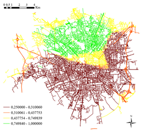 | 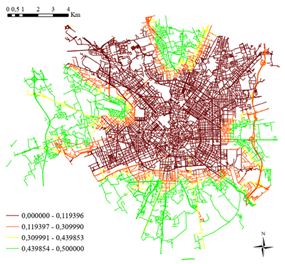 |
| Intensity of Importance (AHP Method) | Linguistic Variables | Triangular Fuzzy Number (l, m, u) | Reciprocal Triangular Fuzzy Number (l, m, u)−1 |
|---|---|---|---|
| 1 | Equal | (1, 1, 1) | (1,1,1) |
| 2 | Weak | (1, 2, 3) | (1/3, 1/2, 1) |
| 3 | Moderate | (2, 3, 4) | (1/4, 1/3, 1/2) |
| 4 | Moderate plus | (3, 4, 5) | (1/5, 1/4, 1/3) |
| 5 | Strong | (4,5, 6) | (1/6, 1/5, 1/4) |
| 6 | Strong plus | (5, 6, 7) | (1/7, 1/6, 1/5 |
| 7 | Very strong | (6, 7, 8) | (1/8, 1/7, 1/6) |
| 8 | Very strong plus | (7, 8, 9) | (1/9, 1/8, 1/7) |
| 9 | Extremely strong | (9, 9, 9) | (1/9, 1/9, 1/9) |
| RC | VD | T | KI | PAC | SAC | AQ | NR | |
|---|---|---|---|---|---|---|---|---|
| RC | (1; 1; 1) | (1/4; 1/3; 1/2) | (1/9; 1/9; 1/9) | (1/3; 1/2; 1) | (1/7; 1/6; 1/5) | (1/6; 1/5; 1/4) | (1/9; 1/8; 1/7) | (1; 2; 3) |
| VD | (2; 3; 4) | (1; 1; 1) | (1/7; 1/6; 1/5) | (1/4; 1/3; 1/2) | (1/5; 1/4; 1/3) | (1/4; 1/3; 1/2) | (1/6; 1/5; 1/4) | (1; 2; 3) |
| T | (9; 9; 9) | (5; 6; 7) | (1; 1; 1) | (4; 5; 6) | (2; 3; 4) | (3; 4; 5) | (1; 2; 3) | (7; 8; 9) |
| KI | (1; 2; 3) | (2; 3; 4) | (1/6; 1/5; 1/4) | (1; 1; 1) | (1/4; 1/3; 1/2) | (1/3; 1/2; 1) | (1/4; 1/3; 1/2) | (2; 3; 4) |
| PAC | (5; 6; 7) | (3; 4; 5) | (1/4; 1/3; 1/2) | (2; 3; 4) | (1; 1; 1) | (1; 2; 3) | (1/4; 1/3; 1/2) | (5; 6; 7) |
| SAC | (4; 5; 6) | (2; 3; 4) | (1/5; 1/4; 1/3) | (1; 2; 3) | (1/3; 1/2; 1) | (1; 1; 1) | (1/4; 1/3; 1/2) | (4; 5; 6) |
| AQ | (7; 8; 9) | (4; 5; 6) | (1/3; 1/2; 1) | (2; 3; 4) | (2; 3; 4) | (2; 3; 4) | (1; 1; 1) | (7; 8; 9) |
| NR | (1/3; 1/2; 1) | (1/3; 1/2; 1) | (1/9; 1/8; 1/7) | (1/4; 1/3; 1/2) | (1/7; 1/6; 1/5) | (1/6; 1/5; 1/4) | (1/9; 1/8; 1/7) | (1; 1; 1) |
| Criteria | Fuzzy Geometric Mean Value | Fuzzy Weights | De-Fuzzified Weights | Normalized Weights |
|---|---|---|---|---|
| RC | (0.27; 0.33; 0.43) | (0.02; 0.03; 0.05) | 0.03 | 0.03 |
| VD | (0.40; 0.52; 0.69) | (0.03; 0.04; 0.08) | 0.05 | 0.05 |
| T | (3.05; 3.88; 4.61) | (0.2; 0.33; 0.51) | 0.35 | 0.32 |
| KI | (0.59; 0.82; 1.15) | (0.04; 0.07; 0.13) | 0.08 | 0.07 |
| PAC | (1.32; 1.77; 2.28) | (0.09; 0.15; 0.25) | 0.16 | 0.15 |
| SAC | (0.92; 1.26; 1.71) | (0.06; 0.11; 0.19) | 0.12 | 0.11 |
| AQ | (2.19; 2.85; 3.64) | (0.15; 0.24; 0.41) | 0.27 | 0.24 |
| NR | (0.23; 0.28; 0.39) | (0.02; 0.02; 0.04) | 0.03 | 0.03 |
| Value_Road | ||||
|---|---|---|---|---|
| ID_Road | Criteria | Criteria × Weight | ||
| Criteria | RC | 000000000096 | 1 | 0.03 |
| VD | 0.25 | 0.0125 | ||
| T | 0.125 | 0.04 | ||
| KI | 0 | 0 | ||
| PAC | 0.136662 | 0.020499 | ||
| SAC | 0 | 0 | ||
| AQ | 0.25 | 0.06 | ||
| NR | 0 | 0 | ||
| IF_000000000096 | 0.162999 | |||
| Criteria Classification Intervals | |||
|---|---|---|---|
| Intelligence phase: natural breaks + manual | Review phase: manual | ||
| Criteria weights | F-AHP | Figure 6 (base case) | 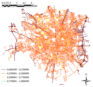 |
| w = 0.125 | 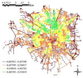 | 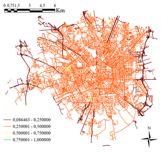 | |
Publisher’s Note: MDPI stays neutral with regard to jurisdictional claims in published maps and institutional affiliations. |
© 2022 by the authors. Licensee MDPI, Basel, Switzerland. This article is an open access article distributed under the terms and conditions of the Creative Commons Attribution (CC BY) license (https://creativecommons.org/licenses/by/4.0/).
Share and Cite
Nodari, C.; Crispino, M.; Toraldo, E. From Traditional to Electrified Urban Road Networks: The Integration of Fuzzy Analytic Hierarchy Process and GIS as a Tool to Define a Feasibility Index—An Italian Case Study. World Electr. Veh. J. 2022, 13, 116. https://doi.org/10.3390/wevj13070116
Nodari C, Crispino M, Toraldo E. From Traditional to Electrified Urban Road Networks: The Integration of Fuzzy Analytic Hierarchy Process and GIS as a Tool to Define a Feasibility Index—An Italian Case Study. World Electric Vehicle Journal. 2022; 13(7):116. https://doi.org/10.3390/wevj13070116
Chicago/Turabian StyleNodari, Claudia, Maurizio Crispino, and Emanuele Toraldo. 2022. "From Traditional to Electrified Urban Road Networks: The Integration of Fuzzy Analytic Hierarchy Process and GIS as a Tool to Define a Feasibility Index—An Italian Case Study" World Electric Vehicle Journal 13, no. 7: 116. https://doi.org/10.3390/wevj13070116
APA StyleNodari, C., Crispino, M., & Toraldo, E. (2022). From Traditional to Electrified Urban Road Networks: The Integration of Fuzzy Analytic Hierarchy Process and GIS as a Tool to Define a Feasibility Index—An Italian Case Study. World Electric Vehicle Journal, 13(7), 116. https://doi.org/10.3390/wevj13070116