Abstract
Autonomous driving has been a topic of great interest in several areas, of which motor racing is no exception. The aim of this work is the autonomous control of the future Formula Student Lisboa vehicle, by implementing different strategies for control and path planning, with the purpose of minimising race lap times. These strategies are tested in simulation, using a realistic model of the prototype. The approach followed involves the decoupling of the lateral and longitudinal subsystems and obtaining the reference path using artificial potential fields, combined with a two-pass algorithm developed to generate a speed profile. In this way, a sub-optimal solution is reached that adequately portrays the expected behaviour of a human driver while respecting traction conditions. The process of generating the speed reference requires prior knowledge of the track layout. This assumption is then eased for obstacle avoidance, i.e., for a scenario where, in addition to the track limits, unknown static obstacles are present. A decoupled control approach is followed controlling each of the two subsystems individually.
1. Introduction
Autonomous electric vehicles have been a topic of growing research and investment in recent decades. They can have a wide range of applications, covering different types of systems (such as small unguided robots or unmanned vehicles) and environments, which can be extended from indoors to outdoors or even to planetary exploration. This autonomy is not just “all or nothing”, but rather a spectrum with six development stages defined by the Society of Automotive Engineers (SAE), where the core competencies needed can be broadly divided into three categories: perception, planning, and control [1]. Whatever the stage and irrespective of the vehicle having a conventional, a hybrid, or an electric engine, its control ought to be designed to improve energy efficiency [2,3,4], which is jeopardised if controllers are poorly conceived.
Perception algorithms allow the vehicle to detect and process the environment and usually make use of the Global Positioning System (GPS), computer vision, and a wide range of sensors [5], which, to compensate for individual shortcomings and achieve a positive redundancy, can be coupled via sensor fusion. From the received data, planning derives instructions for the system, which will act in accordance with the available data; planning is usually categorised as global, behavioural, or local [1,6,7]. Local planning may concern obstacle avoidance [8,9,10], trajectory planning [6,8,11], or path planning [6,12]; the latter frequently involves a decoupled approach regarding the steering and the velocity (see, e.g., ref. [13] for an application to a Formula 1 circuit or [14] for a review of algorithms). Finally, control competency executes the planned actions that have been generated by the previous process. There are usually a lateral controller and a longitudinal controller that handle each of these two movements decoupled from each other; these controllers provide two different input signals: a steering command and an acceleration or a braking signal, respectively.
This paper applies these concepts to an electric Formula Student (FS) car. FS is one of the better-known competitions in an academic-oriented environment: students are challenged to design, build, and test a race car according to a specific set of rules. With the intent of competing in the driverless category introduced in 2017, the Formula Student team from Instituto Superior Técnico—Universidade de Lisboa (FST) is currently developing its first hybrid prototype, in the sense that allows both person-driven and driverless configurations. The methods and results shown in this paper are not limited to the FS car used to illustrate them; they can all be used with a vehicle in a structured environment. While the first Formula Student Driverless competition was won by a car that sought to keep the middle of the track [15], this trivial path planning can be smoothed and improved to achieve shorter distances (as done already by the first robot to win the DARPA Grand Challenge in 2005 [16]). By improving obstacle avoidance, accelerations and decelerations become softer when negotiating narrow passages; consequently, these improvements are expected to help the vehicle travel farther with a full battery charge.
However, the complexity of the underlying algorithms is highly influenced by the scenario into which the vehicle will be inserted. Comparing autonomous city driving with autonomous racing, the degree of unpredictability of the surroundings in the latter is distinctly lower, and this, combined with the highly controlled and regulated environment, allows for simpler approaches regarding perception, which frequently rely on the combination of light detection and ranging (LiDAR) sensors, cameras, and computer vision [17,18]. Planning is usually based on a minimum lap time problem, which accounts for the vehicle dynamics and track boundaries. Finally, the control strategies used in a racing scenario frequently require more data than provided by perception (acquired, e.g., from motor encoders, GPS, or accelerometers) or from estimation [18]. The longitudinal control problem is frequently simplified by assuming that many of the dynamics of the drivetrain, motors, and transmission are regulated by low-level controllers, resulting in a fairly simple system to control [19], or combined with the lateral control for an appropriate model predictive control (MPC) formulation [12]. On the other hand, lateral control tends to include the inertia of the car and tire forces, ranging from models based on the path, which may or may not involve MPC formulation, to models based on vehicle dynamics such as the single-track [20] or four-wheeled [21] models.
As this work mainly focused on improving the planning and the lateral control of the autonomous vehicle pipeline, the objectives are threefold:
- Develop an algorithm for path planning under the assumptions that there is an a priori knowledge of the track layout and an algorithm for online obstacle avoidance considering static obstacles;
- Design different control strategies to effectively steer the vehicle, as well as a low-level controller, in order to obtain more accurate results, ensure vehicle stability, and avoid wheel lock or spin;
- Test, evaluate, and compare the different algorithms, using a developed, realistic model of the vehicle.
This led to the development of path planning and control strategies that are new in FS and suggests the following autonomous racing principles:
- Use the centerline to place the attractive force, to cut the corners while keeping within track;
- Implement decoupled planning (not just decoupled control);
- Deal with obstacle avoidance using transverse forces, to ensure that they are overcome without unduly decelerating the movement and, thus, wasting energy;
- Values for the observation, warning, and danger radius should vary continuously with velocity (using a spline).
The remainder of this work is structured as follows: Section 2 describes the vehicle modelling, Section 3 the planning algorithms, and Section 4 the control strategies; the simulation results are presented and discussed in Section 5, and the conclusions, as well as suggestions for future research on this topic are covered in Section 6. The list of abbreviations is given at the end.
2. Vehicle Modelling
Since in this paper, controller design, tuning, and validation are made resorting to simulation, it is important to have models that emulate the vehicle behaviour. In this section, two categories of vehicle models are detailed: the first, designated as realistic, has a high degree of complexity, being used for simulation; the second, designated as simplified, includes the models used for control and observer design, as well as for preliminary validation. The parameters of the vehicle are given in Table 1.

Table 1.
Vehicle model parameters.
2.1. Realistic Model
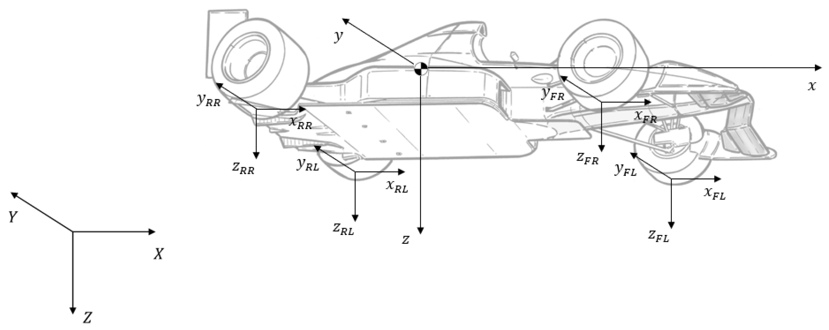
The vehicle model used for simulation has six degrees of freedom (DOF), modelling the vehicle as a rigid body with a simplified vertical suspension system for each wheel [19]. The car is four-wheel driven (4WD) by independent electric motors and front-wheel steered.
To formally describe the vehicle motion, six reference frames are used, namely the global frame—which follows the north-east-down (NED) convention, where X points north, Y east, and Z down—the local reference frame—which coincides with the car’s centre of gravity (CG) with a forwards-right-down alignment—and four additional reference frames attached to the tire contact patches. They are represented in Figure 1.
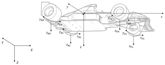
Figure 1.
Reference frames.
The model formulation resorts to a state-space representation where the sixteen states are:
- The linear and angular velocities of the centre of gravity (CG) expressed in the local frame (6 variables);
- The CG position expressed in the global frame (3 variables);
- The Euler angles associated with the rotations from global to local frame (3 variables);
- The angular speeds of each of the four wheels (4 variables).
The inputs are:
- The four wheel torques ;
- The steering angle .
The model returns the sixteen state derivatives and generates as output vectors with four elements (one for each of the four wheels):
- The suspension deformations ;
- The slip ratios ;
- The slip angles ;
- The forces and moments resulting from the tire–ground interaction.
Regarding the kinematics, the linear and angular velocities of the body frame can be expressed in the global frame as
where stands for the transformation matrix from the Euler angles’ rate of change to the CG angular velocities and is the rotation matrix that converts global frame coordinates into local frame coordinates. The expressions for both matrices can be found in [22].
Lastly, with respect to the dynamics, from the Newton–Euler equations, it follows that
where m is the vehicle mass, the gravity vector, and the vehicle’s inertia tensor and wheel rotational inertia, respectively, and R the tire radius. In the above equations, the terms with the subscript represent the resultant force and torque acting on the CG, which includes tire, dissipation, and aerodynamic forces in (3) and energy dissipation in (4). There are four equations given by (5), one per wheel; stands for dissipation torque, and vector collects the values of for each wheel:
All dissipations and aerodynamics forces were modelled in a quadratic form, i.e.,
Powertrain
Due to the complexity of modelling the full powertrain system, a simplification was made in which the motor losses are dynamically modelled, resorting to the implementation of an efficiency map, and all the remaining losses were considered as constant. Additionally, to approximate the torque response dynamics, the first-order system [23]:
was implemented, where is an efficiency to account for the remaining losses and is the time constant for the torque dynamics that accounts for the electrical time constant and mechanical response.
Steering
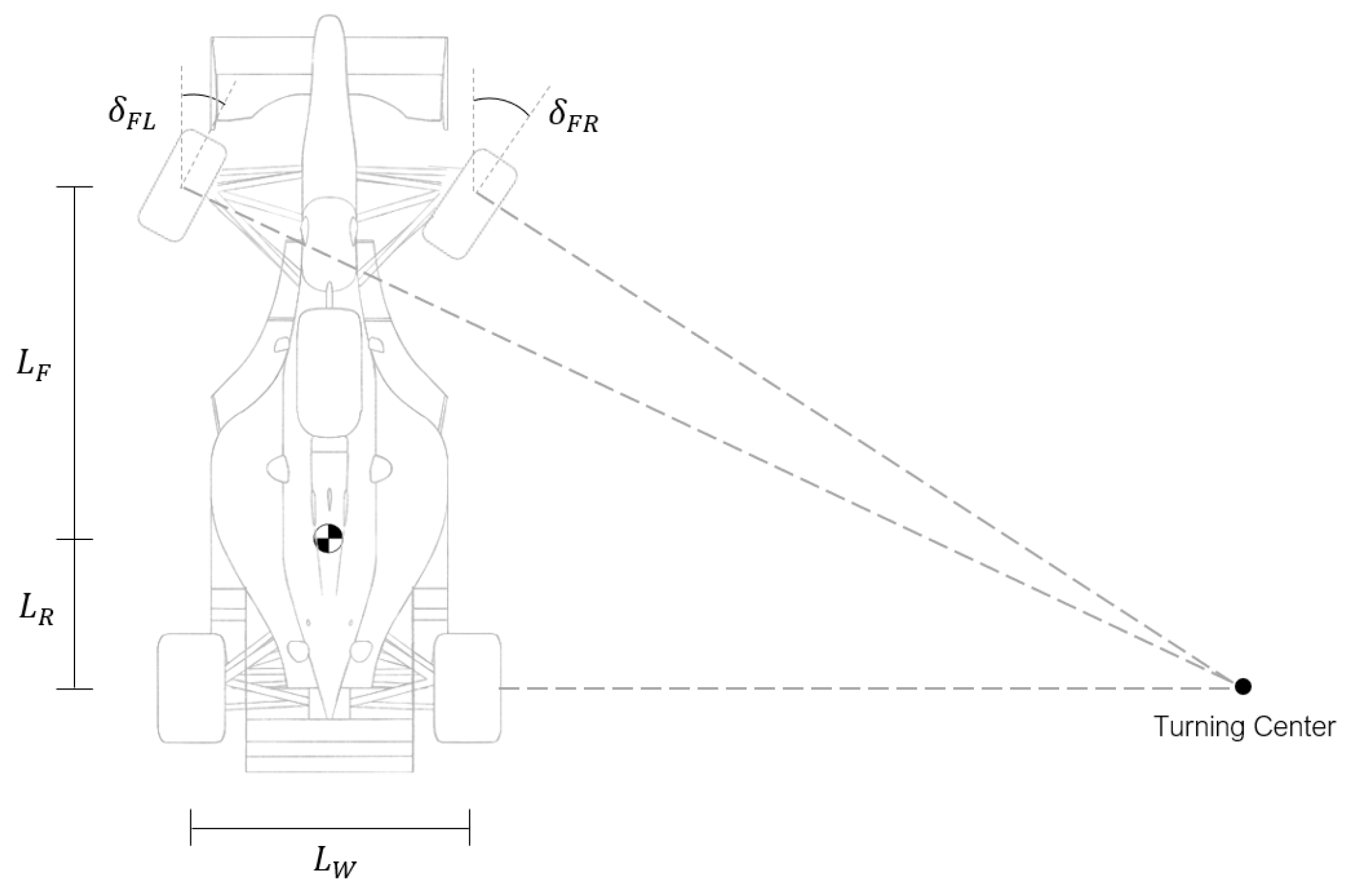
Considering a low-speed or low-curvature cornering manoeuvre, as the vehicle travels along the curved path, all tires follow unique trajectories around a shared turn centre, each one with a specific curvature radius. Hence, to avoid sliding and maintain a pure rolling condition, the angle described by the inside front tire angle must be larger than the one described by the outside front tire, as represented in Figure 2.

Figure 2.
Ackermann steering .
The geometry that allows obtaining such configuration, known as Ackermann steering, computes the steering angles as
in which and are the wheelbase (sum of the distances from the CG to the front axle and from the CG to the rear axle ) and the track width (distance between the two wheels of the same axle), respectively. This geometry was the one considered since low-speed or low-curvature cornering manoeuvres are typically found in FS race tracks.
Similar to the powertrain modelling, a first-order system given by
used in order to model the relation between the real and command steering angles. Here, stands for the steering actuation time constant. Lastly, a slew rate limitation is also implemented to model the physical limit in the actuator speed.
Suspension
A simplified suspension model was used, where each suspension quarter has an equivalent linear spring–damper system that is directly actuated, normal to the ground plane and with punctual contact with the driving surface. For this suspension model, the vertical force is given by
where k and c are the elastic and damping coefficients of the linear spring–damper systems, respectively, and stands for the motion ratio, defined as the ratio between wheel and equivalent spring–damper system displacements (which can be obtained through kinematics relations). This ratio is introduced to correct the fact that the real suspension mechanism is not directly actuated, but through pushrods and bellcranks.
Tires
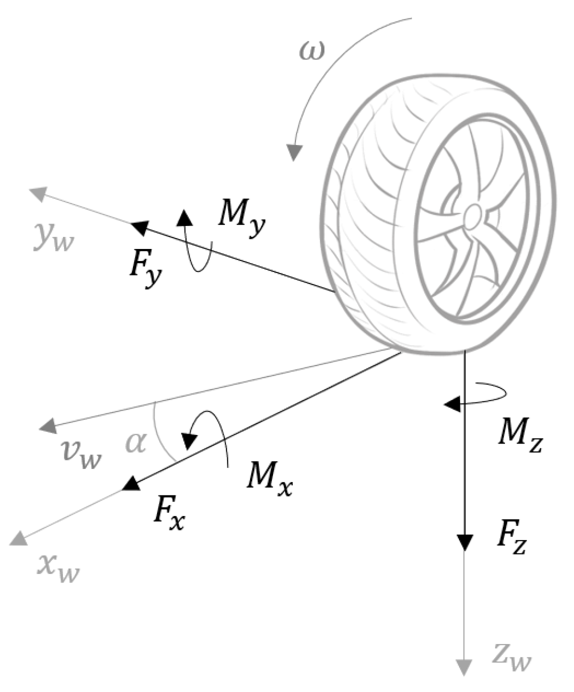
The tires, as the only element interacting with the driving surface, are responsible for the generation of the forces and moments that allow the acceleration, braking, and turning of the vehicle, as represented in Figure 3. Due to the inherent complexity of measuring such mechanical quantities in real time, tire models are commonly used to provide estimations.

Figure 3.
Schematics of a tire and generated forces and moments.
For this work, the Pacejka tire model [24] was considered to be suitable as it is the one used by the FST Lisboa tire supplier. However, to be able to employ the provided tire model and compute the friction loads, several concepts must be defined first.
When a vehicle is in contact with the ground, part of the energy delivered by the motor torque is consumed by friction, generating a longitudinal force , which, opposing the wheel rotation, is responsible for the acceleration and braking of the vehicle. This force is influenced by the slip phenomenon, which can be quantified by the slip ratio [24]:
in which represents the longitudinal component of the linear wheel velocity in the wheel coordinate system. However, it is important to note that, if the vehicle is turning, a lateral force is also generated, which is influenced not by the longitudinal slip, but by the side slip, quantified by the angle presented in (16) [24].
Given the non-uniform tire deformation that occurs in the surface originated by the tire–ground interaction, not only forces, but also moments are generated, such as the self-alignment moment , which depends on the same parameters as the lateral force since it is generated by it.
With these concepts associated with tire mechanics defined, it is now possible to state the formula inherent to the chosen model. Commonly known as the Magic Formula, this model resorts to a semi-empirical formulation [24], to mathematically describe not only both longitudinal and lateral forces, but also the self-alignment moment:
B, C, D, and E are the stiffness factor, shape factor, peak value, and curvature factor, respectively, which are empirically obtained and must respect the relations presented in [24]; and are the vertical and horizontal shifts, and lastly, and are the input (which can be either or ) and output (which can be , , or ) variables, respectively.
2.2. Simplified Models
As can be seen from the previous subsection, the systems of equations of motion are complex and highly nonlinear, which would lead to a complex deduction of the appropriate controllers or estimators. As such, two simplified models were used, which will be presented next. These simplified models were also used to obtain a first insight into the eventual problems, an understanding about the influence of some of the controllers’ gains in the system response—allowing making an initial tuning and steering such tuning in the right direction—and, of course, to verify if a given solution—related to planning or control—works.
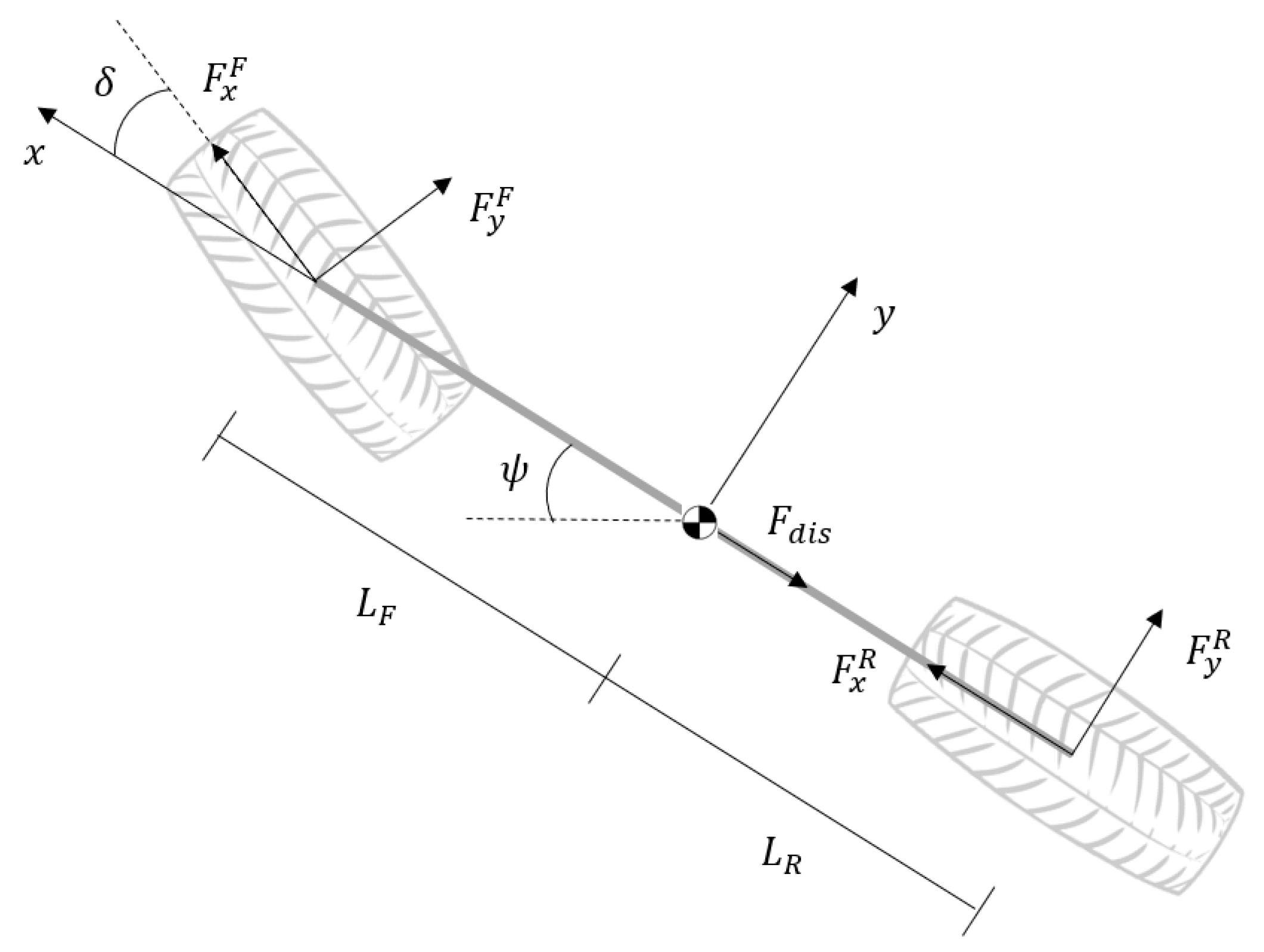
Lateral bicycle dynamic model
In order to develop a model and understand the dynamics involved, the balance of forces and moments plays an important role. Assuming that the vehicle can be seen as a rigid body with planar motion, is rear-wheel driven (RWD) and front steered only, from the lumping of the two wheels belonging to the same axis (inherent to the bicycle model formulation, which has the free-body diagram represented in Figure 4), the dynamics can be described by [23]
where the tire forces and were modelled resorting to the Magic Formula (17), with [18].
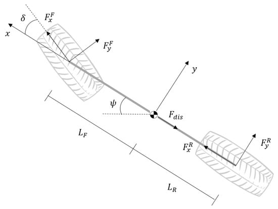
Figure 4.
Free-body diagram for the bicycle model.
For control and estimator design, (19) and (20) were linearised. Let and be the cornering stiffness of the front and rear tires, and let be the position of the vehicle reference point, in the fixed frame, obtained from the integration of
Then, a state-space model can be formulated [21] for the lateral subsystem where the states are , and the dynamic matrix and the input vector are
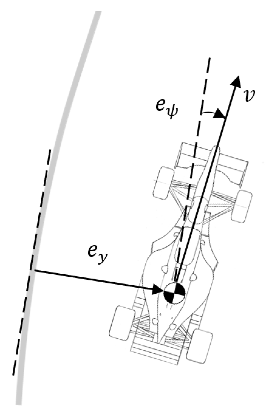
Bicycle dynamic model in terms of tracking errors
A dynamic model with the lateral position and the yaw angle as the degrees of freedom was presented in the previous section. However, it can be useful to define a dynamic model in terms of position and heading errors with respect to the road. These errors are represented in Figure 5 and will be properly defined in Section 4. To formulate such a model, it is only necessary to redefine the linear equations obtained from the previous state-space model in terms of the mentioned errors.

Figure 5.
Position error and heading error in a path-following vehicle. The vehicle reference point is represented as the CG, but another location could also be considered.
The inertial acceleration of the vehicle results from two effects: the acceleration due to motion along the y axis and the centripetal acceleration . Thus, assuming steady-state conditions, the desired acceleration (25) is obtained [21], where can be obtained from the under-steering gradient and wheelbase L through (26) [25]:
With these variables defined, the errors in the lateral and yaw accelerations can be computed as [21]
Substituting (26)–(28) into the equations of the previous model (neglecting both and , and thus further simplifying (26)), a linear state-space can be finally obtained [21], where the state vector is and the dynamic matrix and the input vector are
3. Planning Algorithms
In this section, the algorithms developed for path planning and obstacle avoidance, focused on local planning, are presented.
There are approaches capable of simultaneously optimising both the path and the speed profile [26,27,28]. However, the procedure chosen aims instead to find a speed profile that results in completing a given fixed path in the minimum time [29,30], respecting traction conditions and powertrain constraints.
3.1. Path Planning
For path planning, the employed strategy consists of a decoupled approach, in the sense that one algorithm obtains the path, accounting for the boundaries of the track, and another one regulates its speed. Both algorithms will be described next.
Reference path
The potential field concept, resorting to virtual forces, was used, with the aim of obtaining a reference path more optimised than the centerline, which is the common baseline solution, The main idea behind this approach consists of considering the vehicle as a charged particle moving under the influence of repulsive and attractive potentials. Since the objective is to maintain the vehicle within the track, the repulsive forces will be associated with the track boundaries, the attractive force with a target ahead, and the desired heading (or guidance) with the result of the combination of both effects.
The computation of the attractive force is quite simple, as it only requires the knowledge of the actual position of the car and the selection of a target point lying on the centerline . This force can be mathematically described as [31]
where is a gain, simulating a proportional controller.
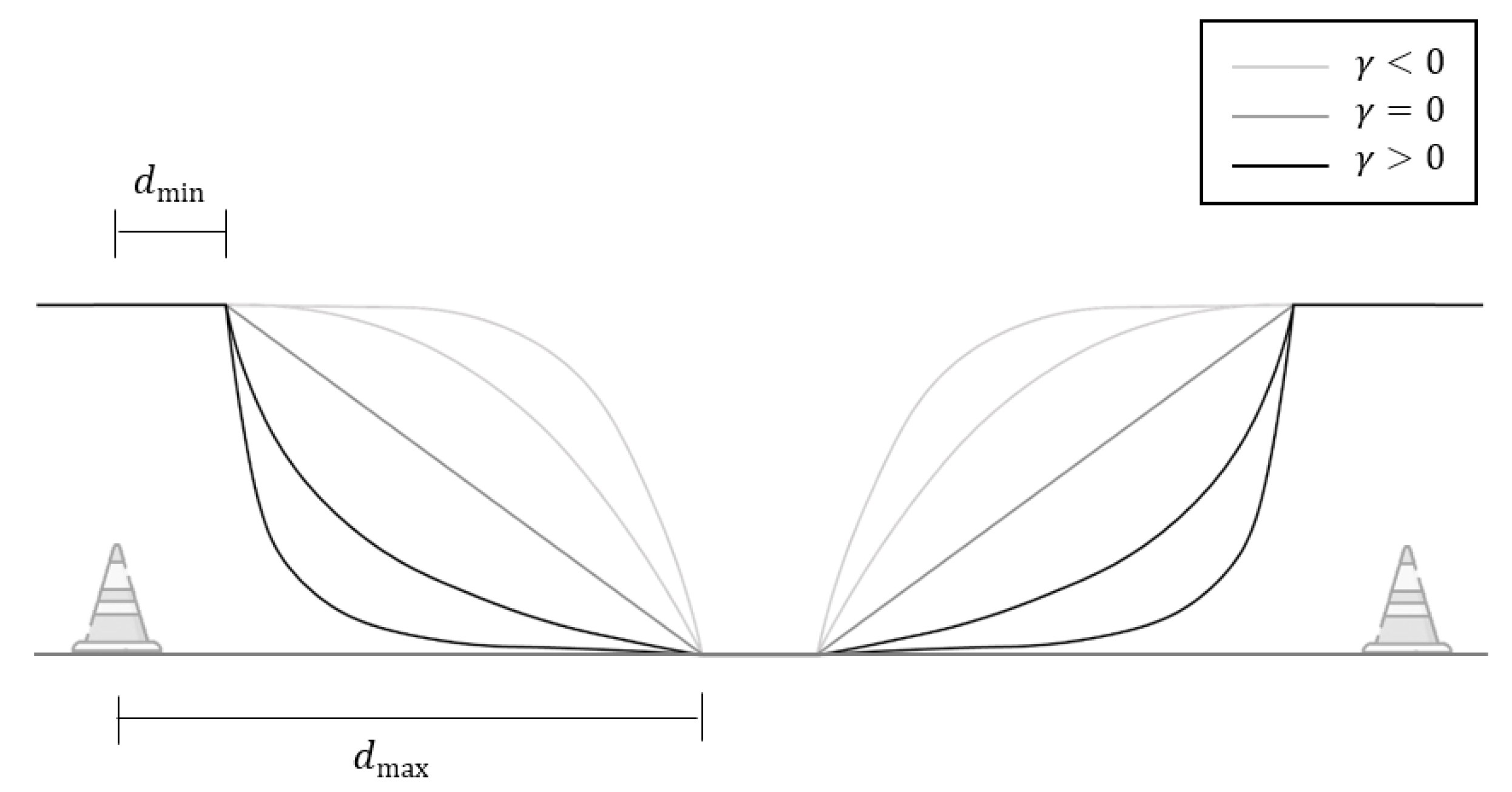
The repulsive force, on the other hand, requires more attention since it depends on the danger level U, which is influenced by the danger of the boundary and the distance between the vehicle’s position and the limits of the track . The danger level U can be given by [31]
where is the distance below which U will be always 1 and the distance above which U will be always 0. Since the value of influences the potential shape—as shown in Figure 6—a positive value was chosen as it allows for a better representation of the expected danger evolution.
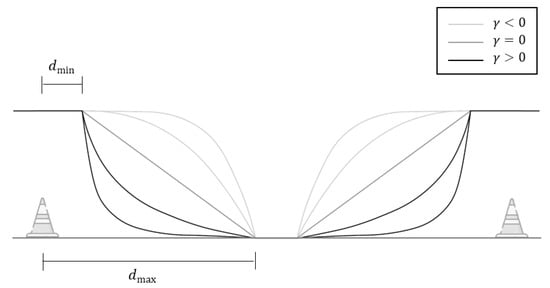
Figure 6.
Evolution of U with d for several values of : the higher the value of , the lower the danger of the boundary. In this figure, two different potential fields are represented, one for each limit. As such, U increases from bottom to top for both limits, but d increases from left to right for the left limit and from right to left for the right limit.
From all the boundary points in the proximity of the vehicle, it is the one with the minimum distance that was selected, since it will present the higher danger level. From this point , the repulsive force can be calculated from [31]
where is a gain, just as in the attractive force.
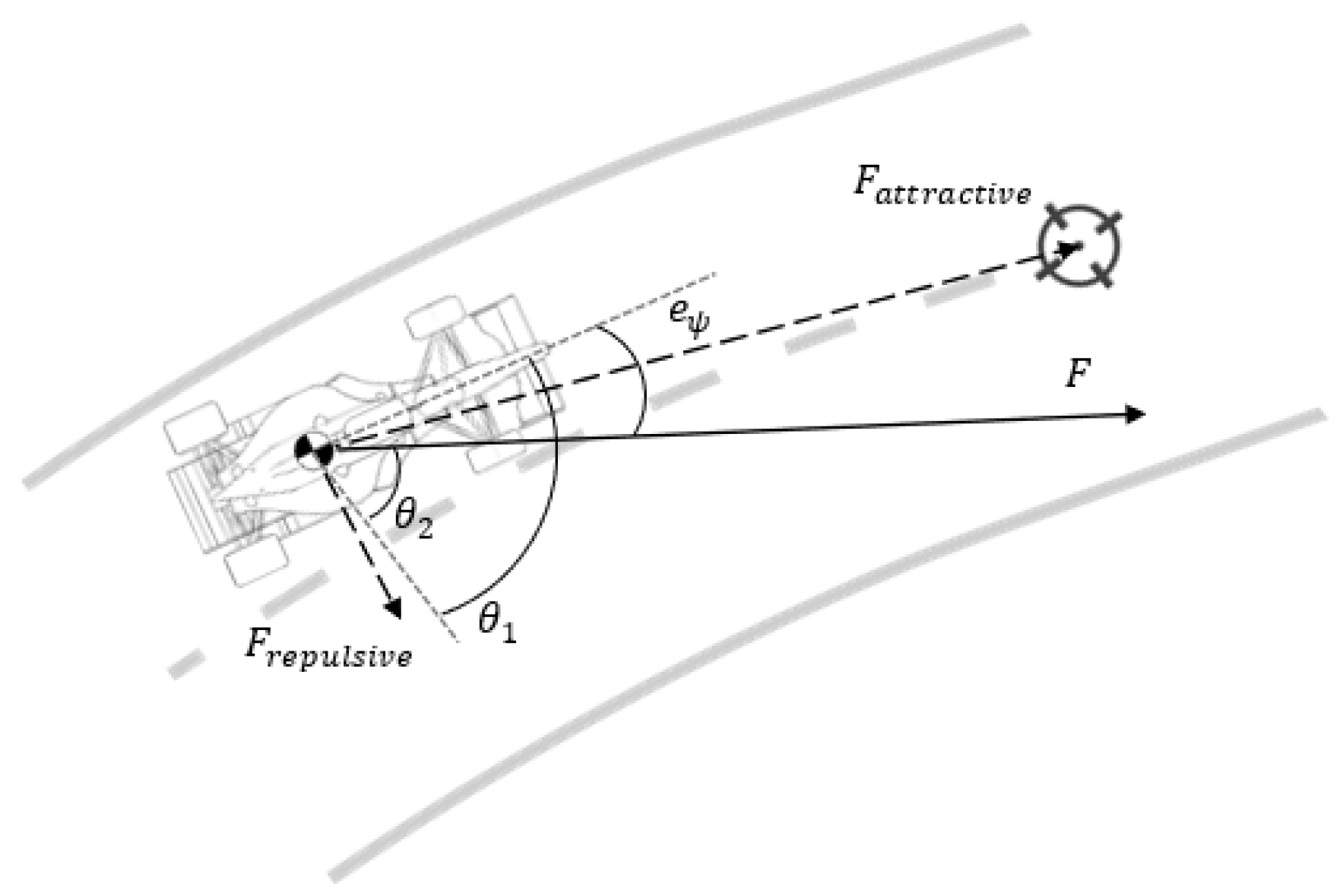
The direction of the virtual resultant force is taken as a desired heading (inasmuch as it minimises the potential). The current heading of the vehicle is known; so, a heading error can be defined as shown in Figure 7. The steering command intends to drive this error to 0, meaning that this is a regulator problem; thus, the steering command was set equal to the error. In this way, the vehicle is steered in the direction of the resultant force. This simple control law can also be described as a unitary proportional controller. However, it should be kept in mind that the reasoning behind the heading error used to obtain this control action involves highly nonlinear calculations.

Figure 7.
Schematic of the forces felt by the vehicle.
Having in mind that an optimal solution cannot be guaranteed, in the sense of guaranteeing the completion of ensuring the completion of a course with the minimum time, this method was further combined with the speed algorithm, which will be presented next, in order to obtain the set of parameters that will result in a solution close to the optimal. These parameters are the distance to the target (which will be referenced as offset), gain , and . The attractive gain was left out and set to a unitary value since, although it can be seen as parameter, it is related to the offset. The procedure adopted in the search of these parameters was a sweeping of the possible range of values, in which, for each of the resultant paths obtained for a constant longitudinal speed of m/s, the speed profile was found. Its variation with the parameters was mostly convex, but with local minima and oscillations, thus demanding a numerical optimisation. Each parameter’s value with the lowest time was chosen as the final one.
Reference speed
Considering an isotropic tire, the maximum transferable force between the road and the vehicle is limited by the tire force, which, using the friction circle model, can be computed from [32]
Neglecting the aerodynamic downforce, the forces in (34) are given by
where K stands for the path curvature, obtained through
In (38), the prime and double prime denote the first and second derivatives, respectively, of the waypoints’ coordinates expressed in the global frame. These derivatives are calculated with respect to the (integer) indexes of the points and can be found using forward, backward, and central differences in the starting, finishing, and remaining points, respectively. As an example, in point 4, .
Discretising the path at N steps, using a fixed step in arc length s, and performing algebraic manipulation of the equations for uniformly accelerated motion:
it is possible to obtain the following equations:
These were the expressions used in the optimisation process. This optimisation is split into two passes, a backward and a forward one, both explained below:
- →
- Backward pass
In the first pass, the backward algorithm determines the maximum speed in turns and the necessary braking distance before each turn. Starting from the finishing point and iterating the sampled curve in the reverse order, the maximum speed at each step is obtained from the minimum between:
- A user-defined limit ;
Once the speed is computed, the negative acceleration required to achieve such a value can be determined with (41), and the minimum between this value and the available negative acceleration by the powertrain (which is given by function h, which will be described latter) is applied. Then, the next iteration continues by moving backward along the curve.
- →
- Forward pass
In the second pass, the forward algorithm maximises the speed and determines the optimal times of transition between acceleration and braking. This is performed reparametrising the original profile using time steps, instead of distance steps, forming a trajectory parametrised in time. Beginning at the starting point and iterating in the forward order, when the velocity is below the velocity profile of the backward pass, the maximum available positive acceleration is applied to increase the speed, and once such velocity is reached, the optimal braking is applied as in the previous pass. As a result, the optimal transition times between acceleration and braking are determined to execute the track in the minimum time and under the acceleration constraints resulting from the traction and/or powertrain.
- →
- Powertrain constraint
From the description provided, it can be seen that both passes use a function h to determine the maximum available longitudinal acceleration in direction , with forward represented as positive. Using K and , such acceleration can be determined from (34) based on the maximum available tire force in the longitudinal direction. However, this value is further limited by the vehicle powertrain.
Assuming that the available torque T can be approximated as constant, but differs depending on the axle and on whether the vehicle is braking or accelerating, the wheel tractive force can be computed from
where is the transmission efficiency and the gear ratio. Thus, the maximum available longitudinal acceleration can then be given by
3.2. Obstacle Avoidance
The algorithm above can be improved, to allow for obstacle avoidance with a priori unknown locations. Static obstacles are presumed given the nature of an FS competition. For obstacle avoidance, a decoupling between the guidance and acceleration was followed once again, as described next. In this scenario, static obstacles are intended to represent other vehicles, which, for simplicity, were modelled as rectangles.
Reference path
An intuitive way of bypassing a given obstacle is to do so through the widest passageway. Resorting again to potential field methods, the algorithm presented in the previous section is again used, considering four main scenarios: the wider passage is free; the wider passage is obstructed; no wider passage is available; no passage at all is possible.
From the definition of the repulsive potential field, given by (32), and knowing that the repulsive force will have a direction perpendicular to the potential field that originated it, some problems can be anticipated, which led to the implementation of four modifications, namely:
- Track limits and obstacles are differentiated, meaning that they are defined by different repulsive fields;
- The obstacles’ repulsive force is forced to have the direction of the vehicle’s closest edge, instead of being perpendicular to the contour lines from the different danger levels;
- The ability to check if a given obstacle was already overtaken is included (when the CG is ahead of all the edges of the rectangle representing that same obstacle);
- The ability to change the repulsive and attractive gains if a collision is predicted (by projecting the current trajectory a fixed distance ahead) is incorporated.
Reference speed
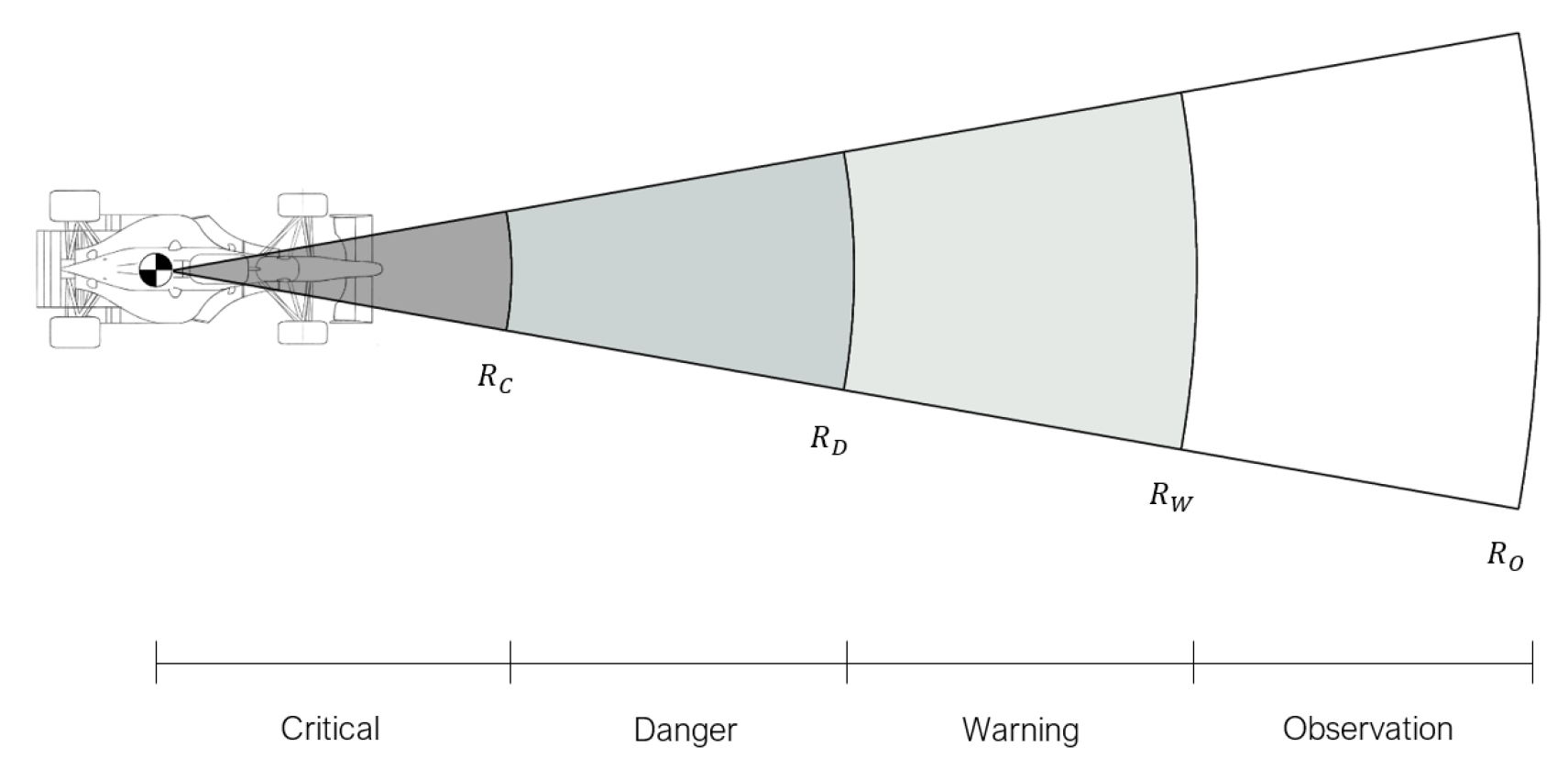
Since the approach followed for path planning requires a priori knowledge about the track to obtain the speed profile, for obstacle avoidance, this reference needs to be obtained with a different method: resorting to the concept of safety zones [33]. However, it should be noted that this method could also be used for path planning if there is no prior knowledge of the track layout.
This approach takes into account that any electromechanical system has an inherent response time, so the ability of a system to respond to a sudden obstacle can be derived from the concept of vehicle safety [33] and translated into the definition of multiple zones within the system observable environment. Such zones are four, as represented in Figure 8, and are responsible for the velocity adjustment needed to avoid obstacle collision.
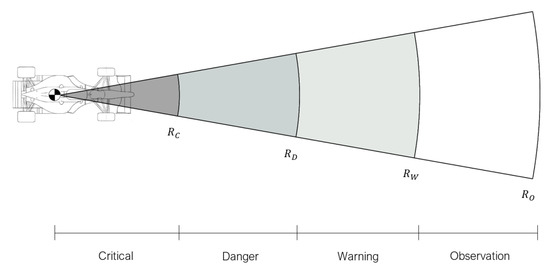
Figure 8.
Schematic of the detection zones.
Similar to what was done for the reference path, some modifications were implemented relative to the concept typically found in the literature [33]:
- Since a negative velocity is not allowed in FS competitions, the profile is changed to take this constraint into account;
- If no possible passage is detected, the reference speed is set to zero;
- Due to possible chattering caused by a linear piecewise profile, a cubic spline interpolation is performed between the different radii, allowing a smooth transition between regions;
- To avoid an “overshoot” in the observation zone, the velocity associated with this outer radius is slightly decreased from the maximum velocity;
- and are parameterised as a function of the velocity, with a linear relation, and not established as fixed values. is fixed, encompassing the vehicle with an extra safety distance.
4. Decoupled Control Approach
We are now in the position to detail the decoupled control already mentioned in Section 3. From the models presented in Section 2, it is possible to observe a coupling between the longitudinal and lateral subsystems. However, considering the torque T and the steering angle as inputs, the linearisation of the bicycle dynamics model, presented in (18)–(20), allows obtaining the following state-space representation:
In this model, the non-null terms of sub-matrices and are not necessary since it suffices to notice that this expression shows clearly a division between two decoupled subsystems: a longitudinal subsystem and a lateral subsystem. The tire slip ratio can be included as an additional state of the longitudinal subsystem; this does not couple it with the other subsystem. Thus, for control purposes, a decoupled approach is followed, developing the lateral and longitudinal controllers independently, as presented in this section.
4.1. Available Sensors and Required Estimations
Control requires information—which can be obtained either through measurement or estimation—about some of the states of the realistic model from Section 2. With respect to guidance, control relies mainly on the detection of the plastic cones defining the limits of the race track (then used to generate the path to follow), usually achieved through cameras, LiDAR sensors, or a combination of both to compensate for individual shortcomings and achieve a positive redundancy.
In what follows, when the reference is found online to provide obstacle avoidance, it is assumed that cameras and LiDAR sensors provide the information needed to navigate in the track outlined by the cones. On the other hand, when the reference is found offline, in advance, information about some states in a fixed coordinate system is needed. Thus, it is assumed that the position of the vehicle in the global frame could be accessed with the fusion of a GPS system with other sensors (since the GPS alone lacks the necessary accuracy) and its orientation resorting to an appropriate compass or gyroscope. Some of the control strategies used in this scenario will require additional information, such as the rate of change of the lateral error , the lateral velocity , and the yaw rate . The latter could be obtained with an inertial measurement unit (IMU); it was assumed that this sensor was not available, and all these three states need to be estimated.
Since we are not here concerned with sensor modelling, sensors were emulated converting the variables in the global frame, obtained from the simulator, into the local frame—the ones provided by the sensors. Considering and the coordinates of a given set of points (which could represent, for example, plastic cones) in the global and local frames, respectively, their relation is
where stands for the coordinates of the local frame origin expressed in the global frame. Thus, from the knowledge of the vehicle’s position and orientation , obtained from simulation, the required transformation to obtain a given point in the local reference frame can be obtained by inverting the rotation matrix in (47) and solving for .
Speed control will require the feedback of the yaw rate , longitudinal speed , and slip ratio , not available from sensors. Although an accelerometer or a speedometer could provide useful information, the accelerometer is sensitive and noisy, so obtaining through integration is inaccurate; due to the presence of longitudinal slip, the angular speed obtained from the speedometer will not correspond directly to the longitudinal speed of the vehicle. Hence, as no sensor could provide information about the slip ratio, both and are not available and should be estimated; it was simply assumed that they were available for feedback.
4.2. Longitudinal Control
As was proposed in [23], a cascade control architecture with proportional gains was used. Such a structure was chosen as it allows controlling the slip ratio and the longitudinal speed (chained variables) separately and performing a direct saturation of the physical quantities that must be limited. In this structure, the inner and outer loops’ variables are the slip ratio and the longitudinal speed , respectively, since the former has faster dynamics.
To take into account the load transfer occurring while the vehicle is describing a turn, a left/right motor torque asymmetry was created, assisting the control of the slip ratios generated in each tire, which is possible due to the use of independent wheel-hub motors. With this in mind, the control law implemented can be mathematically described by [23]
where and can be computed as [23]
and the wheels are numbered as follows: 1, front left; 2, front right; 3, rear left; 4, rear right. The parameters were tuned from the innermost to the outermost loop, in the same manner described in Section 3.1, with values , , , and .
4.3. Lateral Control
Lateral control, related to the ability of steering the vehicle to a different lateral position, frequently relies on the knowledge of the vehicle’s pose regarding the track, or in relation to a given referenced path, resorting to variables typically called path-following errors. As such, in this subsection, these variables will be introduced first and then the control strategies will be presented.
Cross-track and heading errors
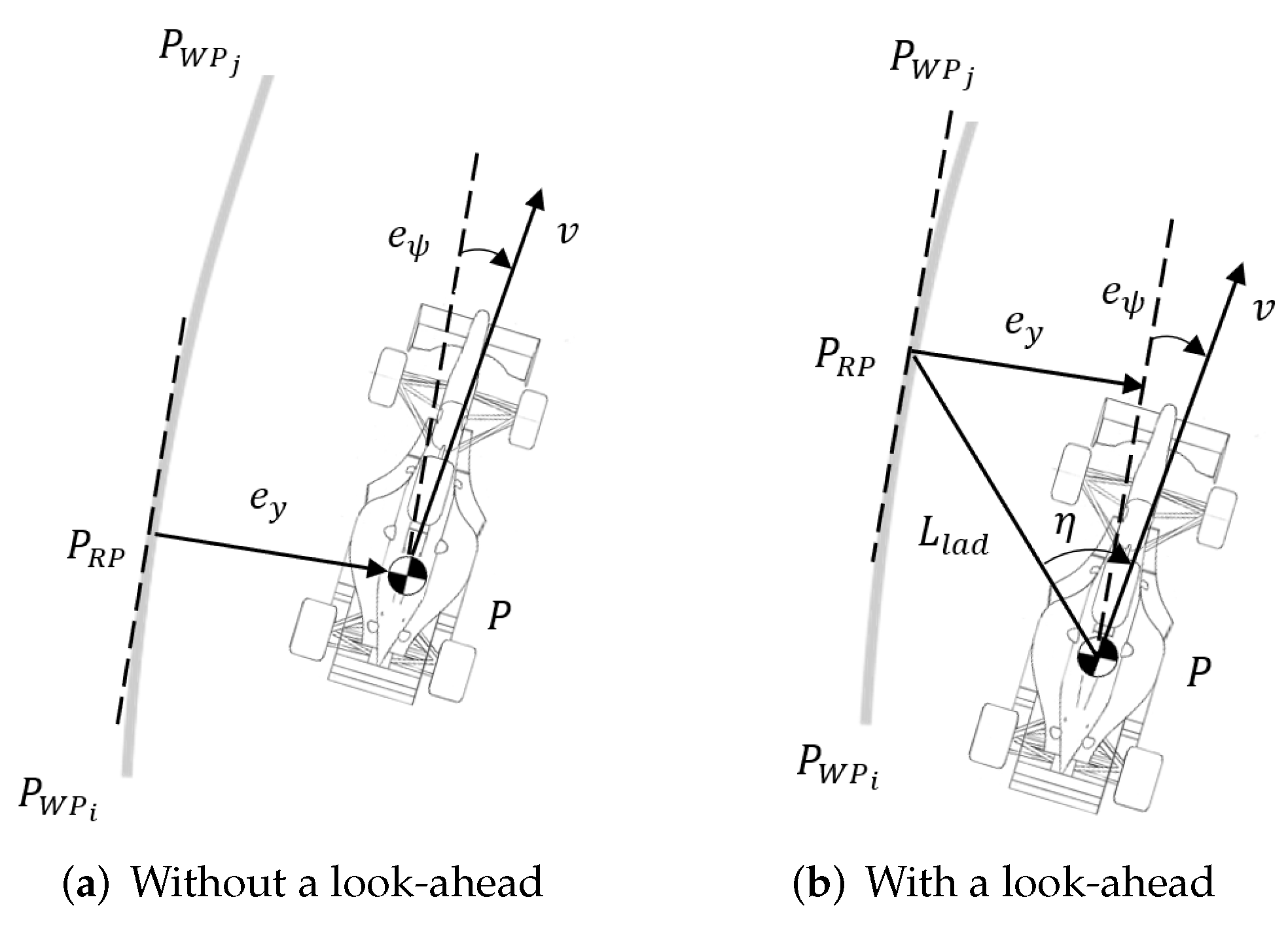
In autonomous driving, it is essential to know the vehicle pose in relation to the track in order to allow the control algorithm to correct eventual errors. These can be related to a distance (such as the cross-track error) or an angle (of which the heading error is an example). While it is possible to define such errors in different manners, in this paper, it was assumed that the vehicle has the waypoints in its front, provided by the perception and planning algorithms, and would then curve-fit them with a second-order polynomial in order to obtain a reference path.
The computation of the path-following errors under this assumption must be done both in the absence and presence of a look-ahead distance , since such a concept is frequently used for control: indeed, it allows for a timely correction of the errors, providing an anticipation capability. Let be the reference point to the car expressed in the local frame and the tangent at that point. The only difference between using or not a look-ahead distance is the location of this point and, consequently, the tangent (as can be seen from Figure 9). Thus, the mathematical expression for the cross-track error and the heading error is the same regardless of the situation. These errors are given by
where the heading error was defined as the angle between the referenced tangent and the vehicle’s velocity vector to take into account eventual sideslip. Because both errors are a cross-product of vectors in the plane, only the z component of and will be different from zero.

Figure 9.
Cross-track and heading errors.
An additional error parameter that will be used in one of the controllers can also be defined. is the angle between the look-ahead vector (which can be obtained once the reference point has been established, since its elements will be equal to the coordinates of such point in the local frame) and the velocity vector, as shown in Figure 9b. This variable can be computed as
and is scalar, for the same reason why errors (51) and (52) are, in practice, scalar as well.
Control strategies:
- →
- Pure pursuit (PP)
The pure pursuit controller [34] consists of a nonlinear control strategy, where only one parameter is utilised as the error: the angle , represented in Figure 9b.
Assuming a kinematic vehicle model and using a circular arc to connect the rear axle of the vehicle to an imaginary point moving along the desired path, this controller calculates the required steering angle from the curvature of such an arc (obtained geometrically, as shown in [34]) through
- →
- Linear quadratic Gaussian (LQG)
The linear quadratic Regulator (LQR) approach is a linear control strategy. It consists of minimising a given quadratic performance index [35], which penalises how far the final state of the system is from zero at the end of a finite time horizon and also penalises the state and control authority evolution during the same time horizon. For this minimisation, a significantly good approximation of the optimal solution can be obtained by solving the algebraic Riccati equation (ARE) [35], which requires establishing two tuning parameters: the state weighting matrix , which penalises the state error, and the control weighting matrix , which penalises the actuation.
Considering the bicycle dynamics model from Section 2, the control law is given by
where the gains are obtained from the ARE. Since the model used is parameterised as a function of longitudinal velocity, these gains will be velocity dependent, making it necessary to update them accordingly. This is done resorting to a gain scheduling, where the gains are calculated offline for the speed operating range and then obtained from a neighbourhood table containing these values.
Since variables and are not accessible directly from sensors, the design of a Kalman filter to estimate them is necessary (hence, the designation of LQG). To obtain the gains related to this filter, two additional parameters are needed, namely the process and sensor noise covariances. This estimator uses the same model as the one used for the LQR and resorts, once again, to a gain scheduling to update the gains.
The weighting matrices for the LQR and Kalman filter are
- →
- Kinematics lateral speed (KLS)
The kinematics lateral speed controller [34] is based on the distance between the vehicle and the reference path and on how such a distance should influence the desired rate of change of the cross-track error : if the car is far from the reference line, it is required to get closer faster than it would get if it were not that far [34]. As such, can be defined as proportional to the cross-track error , with a negative sign. In order to reduce the error between the desired and actual rates of change, the controller must steer the car according to [34]
where and are positive constants and denotes the curvature of the path at the reference point , which can be computed by a different definition from the one presented in (38), since a polynomial was used to curve-fit a given set of waypoints. Let and be the coordinates expressed in the local frame of the n points curve fitted for the reference path generation and the function describing the second-order polynomial used. Then, can be computed as
The lowercase letter k was used, since is computed with respect to the local frame (while in (38), the uppercase K denotes a curvature with respect to the global frame).
The gains used, found with the procedure described above, are and .
This controller (just as MSM below) resorts to a bicycle vehicle model formulated with respect to the path to obtain, from linearisation, a general expression (as in [34]) for the steering angle, which is then used to obtained the control laws.
- →
- Modified sliding mode (MSM)
The sliding mode control strategy is a simple and robust control law, which does not require a precise model of the system [34]. However, due to the discontinuous nature of its control action, this type of control usually leads to oscillations that are commonly designated as chattering, which can then be be weakened or eliminated. As such, as suggested in [34], the sliding surface is defined as (60) and the sliding controller as (61) in order to ensure stability without chattering.
The resulting modified sliding mode control law can be obtained from [34]
where and are weighting coefficients, is the curvature at the reference point computed from (59), and is given by
Since variable is not directly accessible from sensors, a Kalman filter was designed to estimate it. The model used in this estimator is the bicycle dynamics, written in terms of road errors and, similar to what was done in the LQG controller, resorts to gain scheduling to update the gains.
The weighting matrices for the Kalman filter and the remaining gains used are
5. Results and Discussion
Now that the planning algorithms and the multiple control strategies have been presented, both will be evaluated resorting to simulation. The implementation and simulation were performed through the use of Matlab 2020b and Simulink, which are not open-source software. They are widely used to model different types of systems and have plenty of documentation available and community support, these being the reasons why they were chosen. However, alternative open-source options could be used, such as SciLab e Xcos.
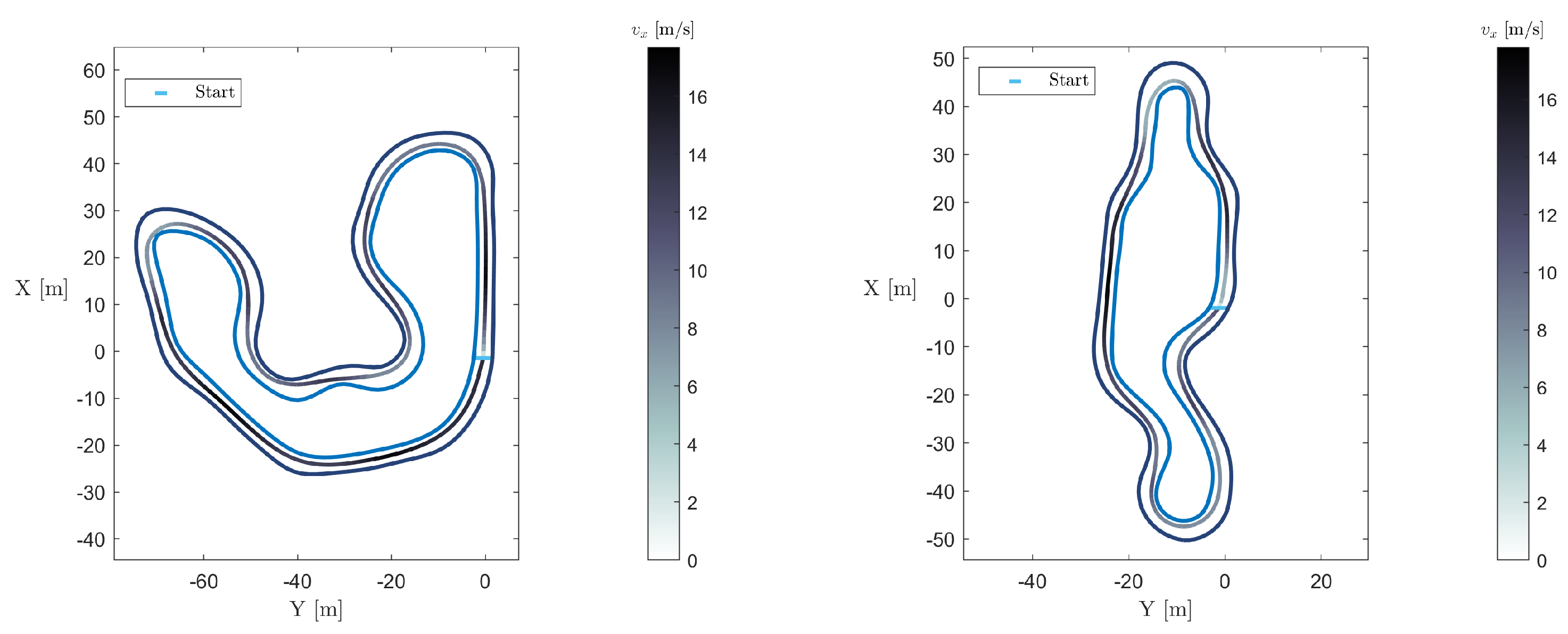
For evaluation purposes, two tracks from the trackdrive event of a Formula Student competition held in Germany (FSG) and Italy (FSI) were used, beginning with path planning. They are shown in Figure 10, along with the corresponding reference trajectories sketched with various colours, which have a correspondence with the values presented in the colour bar.
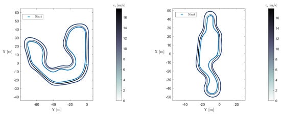
Figure 10.
FSG (left) and FSI (right) reference trajectory.
From the trajectories shown in Figure 10, it can be seen that the vehicle cuts corners while driving slower in corners and faster on straights; so, the final solution captures this reasonable, expected behaviour of a human driver. The parameters tuned to obtain this solution are presented in Table 2.
Table 2.
Planning parameters.
Since the use of the centerline is a typical baseline solution for the reference path, a comparison with this solution is presented in Table 3. From this table, it is possible to conclude that the centerline solution results in a larger total time lap, since saving time from cutting corners is not an option.
Table 3.
Comparison between centerline and the potential field solution.
After obtaining both reference path and speed profiles, the controllers’ performance in the trackdrive event can be evaluated resorting to suitable metrics. Considering that the reference path is intended to represent a solution close to an optimal one, the root mean square (RMS) of the cross-track error was used as an evaluation parameter. This error was computed separately from the one used for path-following, in order to guarantee an independent method to measure the distance to the reference path to be tracked. The distinction between a line from an arc of circumference was arbitrated to be when the curvature of the path between two waypoints has an absolute value below 0.002 m, i.e., a radius above 500 m. Once the curvature of the track is known, error can be computed as
where C and are the centre and radius of the circumference arc, respectively, denotes the displacement vector from waypoint i to waypoint , and the displacement between a waypoint i and the reference point in the car P.
Lastly, noting that some of the implemented control strategies require or could benefit from the use of a look-ahead distance and keeping in mind that such a distance should change with the longitudinal speed, the controllers’ performance was evaluated for two types of look-ahead profiles, namely a linear and a parabolic one:
The parameters in (67) are given realistic values as if the vehicle were human-driven [36]. Therefore, m is the minimum value of the look-ahead distance, s is the estimated human pilot minimum reaction time, and m/s is a reference velocity.
The results for this event are presented in Table 4, where a column was added to provide additional information. This column qualitatively informs if, in the path actually described, the vehicle touched the cones, but still managed to remain in the track (in which, case a penalty is signalled) or if the vehicle did not finish the course (which will be shown as DNF).
Table 4.
Trackdrive results.
Beginning the analysis with the cross-track error, it can be highlighted that the PP, LQG, and KLS controllers have a similar performance; the difference between the MSM and these controllers is not significant (and possibly even lower with further fine tuning). Some tests (not shown for lack of space and reduced relevance) were performed using the centerline as reference path, and it was noted that the cross-track error, in these cases, increased. This can be explained by the general increase of the curvature, making it harder to track with the same precision as in the path used. Regarding the look-ahead analysis, the linear profile enables both controllers to finish the track and allows for a better performance, with respect to the cross-track error. This can be explained due to the influence of the vehicle speed in this predictive distance: the values obtained with the parabolic profile are higher, leading the controllers to correct the vehicle position prematurely and, consequently, losing part of the benefit associated with the look-ahead concept. This is in accordance with the usual intuitive behaviour of a human driver: as the predictive distance depends not only on speed, but also on curvature, it is usually smaller for larger curvatures. This can be better achieved with the linear profile since, in general, this results in lower predictive distances.
Analysing now the obstacle avoidance scenario, the breakpoints used are presented in Table 5, and the results can be found in Figure 11.
Table 5.
Points used for cubic spline interpolation where m/s.
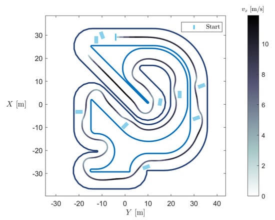
Figure 11.
Described vehicle trajectory in a race track with obstacles.
Regarding steering, the vehicle is still able to portray what can be considered as an expected path, even though some “clumsy” movements can be detected. However, these occur mostly in tight curves and the vehicle still manages to perform well and remain within the track. On the other hand, the behaviour regarding speed presents less flaws, since the speed decreases in the vicinity of an obstacle or in a curve, but increases in straights, as expected. The minimum distances to track limits and obstacles were also computed, and it was found that the vehicle completes the track without touching boundaries or obstacles. However, difficulty in guaranteeing a collision-free trajectory was verified (using other track and obstacle layouts), meaning that the developed algorithm is not straightforwardly generalised.
Concluding, the different control strategies implemented correspond to adequate solutions for vehicle guidance and the planning algorithms are able to provide a satisfactory solution.
6. Conclusions
The results showed that, while the adopted approaches did not guarantee optimality, they were able to portray the expected behaviour of a human driver, and the controllers and path-following strategies provided enabled an FS vehicle to follow a given path, shortening the travelled distance and thus improving energy efficiency.
Some improvements could be implemented in future work. Models for the sensors and the perception algorithms could be included in simulations. A mechanism for the online update should be present since the actual conditions may not match those expected when the reference was generated. A systematic study of the options taken by good FS drivers in the past can give additional clues to the expert decisions embedded in the algorithms. Lastly, for obstacle avoidance, approaches that allow a coupling between the lateral and longitudinal subsystems should be analysed and dynamic obstacles should be considered. A comparison with other strategies that can be applied in an FS competition must include combinations of methods that treat separately path planning (such as the A [37] or the D [38] algorithms) and velocity control. Experimental results are then needed to confirm the correctness of parameter tuning.
Author Contributions
Conceptualisation, S.D.R.S., J.R.A. and M.A.B.; methodology, S.D.R.S., J.R.A. and D.V.; software, S.D.R.S.; validation, J.R.A., M.A.B. and D.V.; writing—original draft preparation, S.D.R.S.; writing—review and editing, J.R.A., M.A.B. and D.V.; visualisation, S.D.R.S.; supervision, J.R.A. and M.A.B. All authors have read and agreed to the published version of the manuscript.
Funding
This work was supported by FCT, through IDMEC, under LAETA, project UID/EMS/50022/2020.
Institutional Review Board Statement
Not applicable.
Informed Consent Statement
Not applicable.
Data Availability Statement
Not applicable.
Acknowledgments
The authors thank Alexandra Moutinho, as well as André Barroso and Alexandre Athayde for all the help and availability given for this work.
Conflicts of Interest
The authors declare no conflict of interest.
Abbreviations
The following abbreviations are used in this manuscript:
| SAE | Society of Automotive Engineers |
| GPS | Global Positioning System |
| FS | Formula Student |
| FST | Formula Student team from Instituto Superior Técnico—Universidade de Lisboa |
| LiDAR | Light detection and ranging |
| MPC | Model predictive control |
| DOF | Degree of freedom |
| 4WD | Four-wheel driven |
| CG | Centre of gravity |
| RWD | Rear-wheel driven |
| PP | Pure pursuit |
| LQG | Linear quadratic Gaussian |
| LQR | Linear quadratic regulator |
| ARE | Algebraic Riccati equation |
| KLS | Kinematics lateral speed |
| MSM | Modified sliding mode |
| FSG | Formula Student Germany |
| FSI | Formula Student Italy |
| RMS | Root-mean-square |
| DNF | Did not finish |
References
- Pendleton, S.; Andersen, H.; Du, X.; Shen, X.; Meghjani, M.; Eng, Y.; Rus, D.; Ang, M.H. Perception, Planning, Control, and Coordination for Autonomous Vehicles. Machines 2017, 5, 6. [Google Scholar] [CrossRef]
- Phan, D.; Bab-Hadiashar, A.; Lai, C.Y.; Crawford, B.; Hoseinnezhad, R.; Jazar, R.N.; Khayyam, H. Intelligent energy management system for conventional autonomous vehicles. Energy 2020, 116476. [Google Scholar] [CrossRef]
- Liu, T.; Hu, X. A Bi-Level Control for Energy Efficiency Improvement of a Hybrid Tracked Vehicle. IEEE Trans. Ind. Inform. 2018, 1616–1625. [Google Scholar] [CrossRef] [Green Version]
- Hall, J.; Bassett, M.; Tate, L.; Hochgreb, S. Energy Efficiency of Autonomous Car Powertrain; SAE Technical Paper; SAE: Warrendale, PA, USA, 2018; p. 2018–1–1092. [Google Scholar] [CrossRef]
- Van Brummelen, J.; O’Brien, M.; Gruyer, D.; Najjaran, H. Autonomous vehicle perception: The technology of today and tomorrow. Transp. Res. Part C 2018, 89, 384–406. [Google Scholar] [CrossRef]
- Gonzalez Bautista, D.; Pérez, J.; Milanes, V.; Nashashibi, F. A Review of Motion Planning Techniques for Automated Vehicles. IEEE Trans. Intell. Transp. Syst. 2015, 17, 1135–1145. [Google Scholar] [CrossRef]
- Schwarting, W.; Alonso-Mora, J.; Rus, D. Planning and Decision-Making for Autonomous Vehicles. Annu. Rev. Control Robot. Auton. Syst. 2018, 1. [Google Scholar] [CrossRef]
- Alcalá, E.; Puig, V.; Quevedo, J. LPV-MP planning for autonomous racing vehicles considering obstacles. Robot. Auton. Syst. 2020, 124, 103392. [Google Scholar] [CrossRef]
- Duhé, J.F.; Victor, S.; Melchior, P. Contributions on artificial potential field method for effective obstacle avoidance. Fract. Calc. Appl. Anal. 2021, 24, 421–446. [Google Scholar] [CrossRef]
- Laurenza, M.; Pepe, G.; Antonelli, D.; Carcaterra, A. Car collision avoidance with velocity obstacle approach: Evaluation of the reliability and performace of the collision avoidance maneuver. In Proceedings of the 2019 IEEE 5th International forum on Research and Technology for Society and Industry (RTSI), Florence, Italy, 9–12 September 2019; pp. 465–470. [Google Scholar] [CrossRef] [Green Version]
- Gerdts, M.; Karrenberg, S.; Müller-Beßler, B.; Stock, G. Generating locally optimal trajectories for an automatically driven car. Optim. Eng. 2009, 10, 439–463. [Google Scholar] [CrossRef]
- Liniger, A. Path Planning and Control for Autonomous Racing. Ph.D. Thesis, ETH Zurich, Zurich, Switzerland, 2018. [Google Scholar]
- Bonab, S.A.; Emadi, A. Optimization-based Path Planning for an Autonomous Vehicle in a Racing Track. In Proceedings of the IECON 2019—45th Annual Conference of the IEEE Industrial Electronics Society, Lisbon, Portugal, 14–17 October 2019; pp. 3823–3828. [Google Scholar] [CrossRef]
- Paden, B.; Čap, M.; Yong, S.Z.; Yershov, D.; Frazzoli, E. A Survey of Motion Planning and Control Techniques for Self-Driving Urban Vehicles. IEEE Trans. Intell. Veh. 2016, 1, 33–55. [Google Scholar] [CrossRef] [Green Version]
- Valls, M.I.; Hendrikx, H.F.; Reijgwart, V.J.; Meier, F.V.; Sa, I.; Dubé, R.; Gawel, A.; Bürki, M.; Siegwart, R. Design of an Autonomous Racecar: Perception, State Estimation and System Integration. In Proceedings of the 2018 IEEE International Conference on Robotics and Automation (ICRA), Brisbane, Australia, 21–25 May 2018; pp. 3823–3828. [Google Scholar] [CrossRef] [Green Version]
- Thrun, S.; Montemerlo, M.; Dahlkamp, H.; Stavens, D.; Aron, A.; Diebel, J.; Fong, P.; Gale, J.; Halpenny, M.; Hoffmann, G.; et al. Stanley: The Robot that Won the DARPA Grand Challenge. J. Field Robot. 2006, 23, 661–692. [Google Scholar] [CrossRef]
- Andresen, L.; Brandemuehl, A.; Honger, A.; Kuan, B.; Vodisch, N.; Blum, H.; Reijgwart, V.; Bernreiter, L.; Schaupp, L.; Chung, J.; et al. Accurate Mapping and Planning for Autonomous Racing. In Proceedings of the 2020 IEEE/RSJ International Conference on Intelligent Robots and Systems (IROS), Las Vegas, NV, USA, 25–29 October 2020; pp. 4743–4749. [Google Scholar] [CrossRef]
- Kabzan, J.; Valls, M.I.; Reijgwart, V.; Hendrikx, H.F.C.; Ehmke, C.; Prajapat, M.; Bühler, A.; Gosala, N.; Gupta, M.; Sivanesan, R.; et al. AMZ Driverless: The Full Autonomous Racing System. arXiv 2020, arXiv:1905.05150. [Google Scholar] [CrossRef]
- De Angelis Cordeiro, R.; Azinheira, J.; Paiva, E.; Bueno, S. Dynamic modelling and bio-inspired LQR approach for off-road robotic vehicle path tracking. In Proceedings of the 16th International Conference on Advanced Robotics (ICAR), Montevideo, Uruguay, 25–29 November 2013; pp. 1–6. [Google Scholar] [CrossRef]
- Kong, J.; Pfeiffer, M.; Schildbach, G.; Borrelli, F. Kinematic and dynamic vehicle models for autonomous driving control design. In Proceedings of the 2015 IEEE Intelligent Vehicles Symposium (IV), Seoul, Korea, 28 June–1 July 2015; pp. 1094–1099. [Google Scholar] [CrossRef]
- Rajamani, R. Vehicle Dynamics and Control, 2nd ed.; Springer: New York, NY, USA, 2012; ISBN 978-1461414322. [Google Scholar]
- Randal, W.; Beard, T.W.M. Small Unmanned Aircraft: Theory and Practice; Princeton University Press: Princeton, NJ, USA, 2012; pp. 30–31. ISBN 9780691149219. [Google Scholar]
- Barroso, A. Traction Control of a Formula Student prototype. Master’s Thesis, Instituto Superior Tecnico, Lisbon, Portugal, 2021. [Google Scholar]
- Pacejka, H.B.; Bakker, E. The Magic Formula Tyre Model. Veh. Syst. Dyn. 1992, 21, 1–18. [Google Scholar] [CrossRef]
- Gillespie, T.D. Fundamentals of Vehicle Dynamics, 1st ed.; Society of Automotive Engineers Inc.: Warrendale, PA, USA, 1992; pp. 196–206. ISBN 9781560911999. [Google Scholar]
- Rucco, A.; Notarstefano, G.; Hauser, J. Computing minimum lap-time trajectories for a single-track car with load transfer. In Proceedings of the 2012 IEEE 51st IEEE Conference on Decision and Control (CDC), Grand Wailea Maui, HI, USA, 10–13 December 2012; pp. 6321–6326. [Google Scholar] [CrossRef]
- Perantoni, G.; Limebeer, D.J. Optimal control for a Formula One car with variable parameters. Veh. Syst. Dyn. 2014, 52, 653–678. [Google Scholar] [CrossRef] [Green Version]
- Lot, R.; Biral, F. A Curvilinear Abscissa Approach for the Lap Time Optimization of Racing Vehicles. IFAC Proc. Vol. 2014, 47, 7559–7565. [Google Scholar] [CrossRef]
- Subosits, J.; Gerdes, J.C. Autonomous vehicle control for emergency maneuvers: The effect of topography. In Proceedings of the 2015 American Control Conference (ACC), Chicago, IL, USA, 1–3 July 2015; pp. 1405–1410. [Google Scholar] [CrossRef]
- Kapania, N.R.; Subosits, J.; Christian Gerdes, J. A Sequential Two-Step Algorithm for Fast Generation of Vehicle Racing Trajectories. J. Dyn. Syst. Meas. Control 2016, 138. [Google Scholar] [CrossRef] [Green Version]
- Valério, D.; Costa, J. An Introduction to Fractional Control; The Institution of Engineering and Technology: Stevenage, UK, 2013; ISBN 978-1-84919-546-1. [Google Scholar]
- Pacejka, H.B. Tire and Vehicle Dynamics, 3rd ed.; Butterworth-Heinemann: Oxford, UK, 2012. [Google Scholar] [CrossRef]
- Casqueiro, A.; Ruivo, D.; Moutinho, A.; Martins, J. Improving Teleoperation with Vibration Force Feedback and Anti-collision Methods. In Proceedings of the Robot 2015: Second Iberian Robotics Conference, Lisbon, Portugal, 19–21 November 2015; Reis, L.P., Moreira, A.P., Lima, P.U., Montano, L., Muñoz-Martinez, V., Eds.; Springer International Publishing: Cham, Switzerland, 2016; pp. 269–281. [Google Scholar] [CrossRef]
- Dominguez, S.; Ali, A.; Garcia, G.; Martinet, P. Comparison of lateral controllers for autonomous vehicle: Experimental results. In Proceedings of the 2016 IEEE 19th International Conference on Intelligent Transportation Systems (ITSC), Rio de Janeiro, Brazil, 1–4 November 2016; pp. 1418–1423. [Google Scholar] [CrossRef] [Green Version]
- Ogata, K. Modern Control Engineering, 5th ed.; Prentice Hall: Hoboken, NJ, USA, 2009. [Google Scholar]
- Droździel, P.; Tarkowski, S.; Rybicka, I.; Wrona, R. Drivers’ reaction time research in the conditions in the real traffic. Open Eng. 2020, 10, 35–47. [Google Scholar] [CrossRef] [Green Version]
- Dolgov, D.; Thrun, S.; Montemerlo, M.; Diebel, J. Practical search techniques in path planning for autonomous driving. In Proceedings of the First International Symposium on Search Techniques in Artificial Intelligence and Robotics—STAIR-08, Chicago, IL, USA, 13–14 July 2008; pp. 32–37. [Google Scholar]
- Stentz, A. Optimal and efficient path planning for partially-known environments. In Proceedings of the 1994 IEEE International Conference on Robotics and Automation (ICRA), San Diego, CA, USA, 8–13 May 1994; pp. 3310–3317. [Google Scholar]

Publisher’s Note: MDPI stays neutral with regard to jurisdictional claims in published maps and institutional affiliations. |
© 2022 by the authors. Licensee MDPI, Basel, Switzerland. This article is an open access article distributed under the terms and conditions of the Creative Commons Attribution (CC BY) license (https://creativecommons.org/licenses/by/4.0/).