Abstract
Rolling-element bearing fault diagnosis has some problems in the applied environment, such as low signal-to-noise ratio, weak feature extraction, low efficiency of feature learning and the complex structure of diagnosis models. A fault diagnosis method based on the comprehensive index method, complete ensemble empirical mode decomposition with adaptive noise independent component analysis (CEEMDANICA) and two-dimensional convolutional neural network (TDCNN) is proposed. Firstly, the original vibration signal of the bearing is preprocessed by CEEMDANICA, and the ICA components with different frequencies are obtained. Secondly, the ICA components are selected as the sample set by using multiscale permutation entropy, correlation coefficient, kurtosis and box dimension. Finally, the sample set are trained and tested by a DCNN model to realize the fault diagnosis of different bearing fault types. In order to verify the reliability of the method, a bearing fault vibration monitoring platform for an electric vehicle two-speed automatic transmission was built to collect the bearing vibration signals of multiple fault types under different working conditions. The diagnostic accuracy of several deep learning models is compared. The results show that the proposed method can realize the single and compound fault diagnosis of rolling-element bearings in an automatic transmission, with a high degree of accuracy.
1. Introduction
New energy vehicles are an important development in industry to achieve the goal of carbon peak and carbon neutralization in China. Battery electric vehicles can get rid of oil dependence, optimize the energy structure, and promote the achievement of the “double carbon” goal. It has become a key research topic in the field of new energy vehicles. Within the development of electric vehicles, the electric drive system with a single gear reducer has obvious shortcomings in the middle and rear acceleration power, high-speed cruise economy and the high-efficiency interval of the motor. Therefore, the development of a two-speed or even multi-speed transmission has become the major research direction for the electric drive system.
The high-speed and constant torque output characteristics of the motor bring more severe working conditions to the transmission gears, bearings and other rotating machinery parts. For the rolling-element bearings of the automatic transmission of electric vehicles, extracting the fault features accurately and diagnosing faults efficiently is of great significance to the operation and maintenance of the vehicle transmission system.
At present, the fault diagnosis methods include temperature analysis [1], acoustic emission detection [2] and vibration analysis, of which vibration analysis is the most widely used. Different preprocessing methods are used to demodulate vibration signals [3], or deep learning models are used for pattern recognition [4]. A multiscale convolutional capsule network (MCCN) is proposed, integrating low-level and high-level features in a convolutional neural network (CNN). It is conductive to noise reduction and robust feature extraction [5]. To solve good sparse representation, a novel deep and shared dictionary learning (DSDL) is proposed, which has the deep structure from deep learning and shared structure [6]. Zhou et al. [7] synthesized a deep convolutional generative adversarial network (DCGAN) which can enable a high diagnosis accuracy with scarce labeled data.
Due to the fact that transmission vibration comes from different sources, fault feature extraction is an important area of research. Since the empirical mode decomposition (EMD) algorithm was proposed, researchers have applied it to the fault diagnosis of rotating machinery and have obtained some notable achievements.
Wang et al. [8] combined EMD with manifold learning, which greatly suppressed the fault of independent components and residual noise while retaining the real fault-related signals. Ziani et al. [9] integrated EMD, Teager–Keiser energy operator and impact detector to realize fault detection in bevel gears under variable working conditions. In order to solve the problem of effective signal and noise mixing in high-frequency signals, Ge [10] and others proposed a fault diagnosis method combining ensemble empirical mode decomposition (EEMD), wavelet semi-soft threshold signal reconstruction and multiscale entropy with support vector machine (SVM). A method based on integrated EMD, permutation entropy (PE), linear discriminant analysis and the Gath–Geva clustering algorithm is adopted, which improved the intra-class compactness of clustering results of fault identification methods [11]. EEMD is used to process non-linear and non-stationary signal data, SVM is used to classify the mechanical state of a small number of signals, and the genetic algorithm is adopted to expand data and feature selection for improving the accuracy of rotor faults identification [12]. Li et al. [13] adopted EEMD and energy moment to extract features, and combined these with a self-organizing feature mapping network, to rapidly and accurately realize the fault diagnosis of motor rolling-element bearings.
In order to improve the reconstruction error of EEMD, complete ensemble empirical mode decomposition with adaptive noise (CEEMDAN) has been used by researchers for data processing.
Xiao et al. [14] compared the effects of CEEMDAN and EEMD on extracting fault characteristic frequency, and proved that CEEMDAN has a better ability to retain the original signal and eliminate noise. Vanraj et al. [15] used CEEMDAN to realize the fault diagnosis of simulated local defects through the sound signal of the gearbox. In order to better extract the weak impulse response from strong noise and heavy interference signals, Huang et al. [16] proposed a bearing fault diagnosis method based on CEEMDAN, periodic segmented matrix and singular value decomposition. In order to solve the problem that the intrinsic mode function generated by EEMD contains residual noise and the internal mode function is difficult to average after adding different Gaussian white noise, Lei et al. [17] proposed a fault diagnosis method based on CEEMDAN and a neural network.
With the application of independent component analysis (ICA) in signal processing, research scholars have combined it with fault diagnosis and made some achievements. Hu et al. [18] introduced EMD FastICA to extract and classify features in the fault diagnosis of wind turbine rolling-element bearings. In view of the problem that the vibration signal of actual engineering is interfered with by strong noise, Lu et al. [19] proposed a method combining single channel ICA and fractal analysis to reduce the impact of noise on the time-frequency analysis of vibration signals. Song et al. [20] used empirical wavelet transform and ICA methods to reduce the noise of vibration signals, which improved the difficulty of early bearing fault feature extraction in low signal-to-noise ratio environments.
Based on the above research, aiming at the problems of noise interference in IMF components after CEEMDAN decomposition and the low classification and diagnosis accuracy of rolling-element bearings, a fault diagnosis method of CEEMDANICA and DCNN based on the comprehensive index method is proposed. First, CEEMDANICA is used to process the original vibration signal to obtain ICA components in different fault states. Then, these ICA components were screened to form the training sample sets through multiscale arrangement entropy, correlation coefficient, kurtosis and box dimension indicators. Finally, the accurate identification of different rolling-element bearing fault types is realized through the training and testing of the DCNN model.
This paper is organized as follows: the current status of fault diagnosis research is presented in Section 1; Section 2 introduces the vibration signal preprocessing method of CEEMDANICA and the classification diagnosis neural network model of TDCNN; The source of bearing failure test data is presented in Section 3; Section 4 introduces the diagnosis process and experimental result comparison analysis of transmission bearing compound fault; Section 5 contains the conclusions.
2. Methods
2.1. CEEMDANICA Method Introduction
To be directed against the problems of modal aliasing in EMD decomposition and residual noise in IMF after EEMD decomposition, Hou et al. [11] added different white noise to different IMF components and proposed the CEEMDAN algorithm, which has the advantage of a small reconstruction error, and which greatly alleviated the problem of IMF quantity uncertainty after adding noise. For the components IMF1, IMF2, … IMFn obtained from CEEMDAN processing, some components still contained noise. In the practical applied environment of bearing faults, there are multiple noise sources from gears and other bearings in the vehicle transmission. At the same time, the compound bearing faults are included, so it is necessary to further extract the features of multiple signal components. The original signal is masked by the medium and low-frequency high-energy noise, so that the independent source signal cannot be obtained. In view of this situation, the signal preprocessing method of CEEMDANICA is proposed. The process is as follows:
If there is an operator Uj(·), it is used to solve the jth IMF of a signal through EMD decomposition.
White noise is assumed ωi, and the range of ωi is 0 to 1. Noise with an amplitude coefficient of εk is added during the EMD decomposition.
X(t) represents the original signal to be decomposed by CEEMDAN. The basic steps are as follows:
1. Add white noise to the original signals to obtain X(t) + ε0ωi(t), the average value of the first IMF component can be obtained by EMD decomposition, and it is recorded as IMF1, and described as:
2. According to the above formula, the residual components are:
3. , i = 1,2, … I, is decomposed by EMD and averaged to obtain the second component.
4. For k = 2, … K, the kth residual component is:
5. i = 1,2, …, I, is operated by EMD, and average kth IMF.
6. Repeat steps (4) and (5) until there are less than two extreme values of the residual component, and record as,
where, K is the total amount of IMF, and the original signal can be expressed as:,
7. For IMF1, IMF2, … IMFn obtained by the above formula, some components are still mixed with residual noise. ICA is used to process these components again and treat each IMF as a mixed signal. Let h1, h2, … hk = IMF1, IMF2,… IMFk, and the matrix can be expressed as:
8. If there is I(t) = [I1(t), I2(t), …, In(t)]T, I(t) is assumed to be a matrix composed of a group of mutually independent signal sources, and W(t) = [W1(t), W2(t), …, Wn(t)]T, W(t) is composed of independent signal sources in I(t), which can be shown as follows:
where (t) is the observation matrix, A is the mixed coefficient matrix, and A is the full rank M × N (m ≥ n) matrix.
9. When S(t) and A cannot be obtained by traditional means, The separation matrix M can be obtained by FICA which can be shown as follows:
where Y(t) = [y1(t),y2(t), …, yn(t)]T is the estimation of the source signal I(t). Repeat the above steps until all independent source signals, called ICA1, ICA2… ICAn, which constitute IMF components are decomposed.
2.2. Comprehensive Index Method
2.2.1. Multiscale Permutation Entropy (MPE)
The characteristic information of complex systems exists in the time series in the form of multiple scales. However, when detecting time series, permutation entropy (PE) can only detect randomness and complexity on a single scale. If there is a time series X = {x(1), x(2), …, x(N)}, yj(s) is obtained after the coarse graining operation. The expression is:
where s is the scale factor and S = 1, 2, …. [N/s] takes the integer value. when s = 1, the original sequence can be expressed by coarse-grained sequence. The MPE can be obtained by calculating the permutation entropy of each coarse-grained sequence yj(s).
2.2.2. Box Dimension
Box dimension and correlation dimension are usually used in mechanical fault diagnosis. The solution of correlation dimension is complex, while the research of box dimension is mature and widely used. It can reflect the dynamic structure change of the dynamic system as a whole, and improve the accuracy of feature extraction. The fault feature extraction by box dimension can be summarized by the following process:
1. It is assumed that the discrete signal yi⊂y, y is a closed set on Rn. Use as thin as possible ε Grid division, N(ε) is the minimum number of meshes covered by the set y.
2. Gradually enlarge the grid to a scale of kε,
where i = 1, 2, … N/k, k = 1, 2, … M. N is the number of sampling points. M < N.
3. The number of calculation grids can be obtained from the following formula:
where N(kε) > 1.
4. A section of scale-free area is selected in the figure lgkε-lgN(kε), and k1 and k2 are the starting point and the end point, respectively, and have a good linear relationship.
5. The slope of the straight line is obtained by the least square method:
6. The box dimension DB is:
2.2.3. Correlation Coefficient
In order to better characterize the correlation between the original signal and the ICA component, the correlation coefficient is introduced. According to the product variance method, the dispersion between the original signal and the average value of ICA components is calculated. Finally, the correlation coefficient is obtained by multiplying the dispersion between each component and the original signal. The expression is:
where, Cov (M, N) represents the covariance between M and N. Var|M| and Var|N| represent the variance of M and N. The larger the value of Var|M, N|, indicates the greater the correlation between M and N, and vice versa.
2.2.4. Kurtosis
Kurtosis K is a dimensionless parameter that measures the impact degree in the signal. It has nothing to do with the parameters of the bearing itself or the operating conditions, so it is widely used in the fault diagnosis of rotating machinery. The formula can be expressed as:
2.3. Two-Dimensional Convolutional Neural Network
Convolutional neural network is a typical feedforward neural network, which is composed of the convolution layer, the pooling layer, the full connection layer and the output layer.
Convolution layer: the function of a convolution layer is to perform convolution operation through different convolution cores, which is a matrix, also known as a convolution filter. Different sizes of receptive fields are obtained by convolution kernels of different sizes, and the output characteristic matrix is obtained by the activation function. Convolution function is as follows:
where: is the jth element of the lth layer; is the ith element of layer l − 1; is the weight matrix of the convolution kernel; is offset. f (*) is the activation function. The convolutional neural network model in this paper adopts the ReLU activation function, and the expression is as follows
Pooling layer: also known as the down sampling layer, pooling is divided into average pooling and maximum pooling. This model adopts average pooling, and the calculation result can be expressed by Formula (20).
The feature learning ability of the model can be greatly improved, and the high-precision identification and diagnosis of various types of bearing faults can be realized through the reasonable design of the convolutional neural network model. In this paper, a two-dimensional convolutional neural network (TDCNN) model is proposed to diagnose the time domain signal of the rolling-element bearing of the automatic transmission. The vibration signal is reconstructed into a 40th order sample matrix forming the input layer. In order to effectively extract the early fault feature information, the convolution kernel size of the first layer is half of the order of the input layer matrix. The step size is set to 1 to enhance the fault signal characteristics.
Based on the above ideas, the structure adopted in this paper is: input layer → convolution layer → pooling layer → convolution layer → pooling layer → full connection layer → softmax classifier.
The structure of TDCNN is shown in the Figure 1.
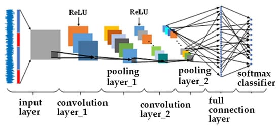
Figure 1.
two-dimensional convolutional neural network model.
The specific parameters of the TDCNN structure are shown in Table 1. The initial learning rate is 0.01, the momentum value is 0.9, the offset is 0, the number of batch processing matrices is 100, the ratio of training samples to test samples is 4:1, and the model iterations are 100 times.

Table 1.
Structure parameters of TDCNN.
3. Bench Vibration Test of Rolling Bearing of Automatic Transmission
Taking the two-speed automatic mechanical transmission as the application object of the bearing fault, the rolling-element bearings with a single fault and a compound fault are manufactured. The bearing with different fault types is installed at one end of the intermediate shaft, and the vibration signal is collected in the comprehensive performance test bench of three motors.
3.1. Two-Speed Automatic Mechanical Transmission
The two-speed automatic mechanical transmission power assembly is composed of the first gear driving and driven gear, the second driving gear and driven gear, the differential pinion, the differential gear ring, the differential, the input shaft, the intermediate shaft, the parking mechanism, the shift motor, the parking ratchet and the rolling-element bearing.
The two-speed transmission prototype and the internal structure of the transmission are shown in Figure 2a,b, respectively.
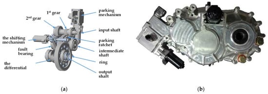
Figure 2.
The two-speed automatic mechanical transmission: (a) Structural diagram; (b) Transmission prototype.
3.2. Test Platform
The three-motors power system performance test bench is composed of a driving motor, two loading motors, a speed increase gearbox, a test piece support, speed sensors, torque sensors, a cooling device and a computer control system. The automatic transmission is bolted to the tooling plate bracket of the test bench. The driving motor and the loading motor can flexibly adjust the axial and longitudinal positions according to the center distance. The test platform is shown in Figure 3.
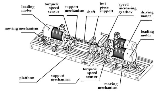
Figure 3.
Two-dimensional schematic diagram of test platform.
3.3. Signal Acquisition
In order to simulate different pitting states of bearings, electrical discharge machining technology is used to prefabricate 7 types of bearing faults, including single pitting failure of inner and outer rings and rolling elements, composite pitting failure of inner and outer rings, composite pitting failure of inner ring and rolling elements, composite pitting failure of outer ring and rolling elements and normal bearing. Among them, the diameter of the severe pitting fault is 0.53 mm, the diameter of the composite fault is 0.18 mm, and the depth is 1 mm. Bearings with different fault types are shown in Figure 4.
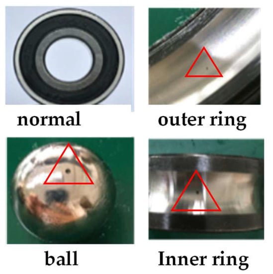
Figure 4.
different types of fatigue pitting bearings.
During the experiment, different rotational speeds and torques were set for the driving motor. The rotational speeds of the input end were 1965 r/min, 2088 r/ min, 2228 r/min and 2366 r/min, respectively, and the torque was 32 Nm. The speed and torque of the input end and output end were fed back in real-time through the speed sensor and torque sensor on the bench. Sensors were arranged on the housing to collect vibration signals from the bearings on the input shaft and the intermediate shaft, as shown as Figure 5.
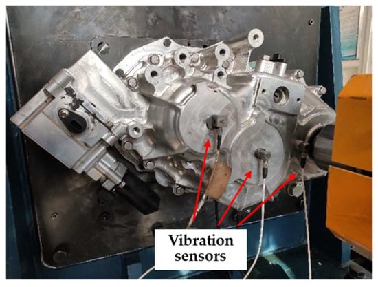
Figure 5.
Arrangement of vibration sensor.
The Siemens LMS vibration signal acquisition system was adopted for data acquisition and storage, as shown in Figure 6. The sensor sensitivity of the fault bearing was 10.03 mV/g in X direction, 9.77 mV/g in Y direction and 9.75 mV/g in Z direction. The computer control system was used to drive and load the motor, and the operation of the platform was observed in real-time. After each group of working conditions was stable, the data acquisition was started. The acquisition time of each group of vibration signals was 30 s. The sampling frequency of vibration signals was 16384 Hz. The Z channel was selected when analyzing and processing the vibration signal. Details of vibration signal data collected in the experiment are shown in Table 2.
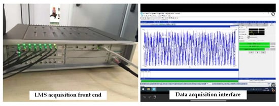
Figure 6.
Acceleration sensor LMS acquisition front end and real-time data feedback.
Table 2.
Description of experimental data set.
4. Fault Diagnosis of Rolling-Element Bearing of Automatic Transmission
4.1. Signal Processing Based on CEEMDANICA
The data from each rolling-element bearing was composed of 10,000 data points from low to high according to four kinds of rotational speeds, which were processed by CEEMDANICA, and ten ICA components were obtained. The ICA component of the inner ring with the severe fault after pretreatment is shown in Figure 7. Taking the severe fault of inner ring as an example, the MPE, kurtosis, box dimension and correlation coefficient of ten ICA components were calculated. Table 3 for the calculation results.
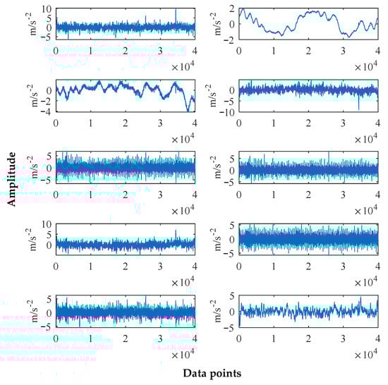
Figure 7.
Ten ICA components after CEEMDANICA for severe inner ring fault.
Table 3.
Index values of different ICA components.
Among the 10 ICA components, the six selected components had the largest eigenvalues of the four indicators. After comprehensively considering the influence of each index, six ICA components of ICA1, ICA2, ICA5, ICA7, ICA8 and ICA9 were selected as the TDCNN model sample set in order of decreasing size from large to small.
4.2. Fault Diagnosis of Rolling-Element Bearing Based on TDCNN
When processing the bearing vibration signal, the local coverage method was adopted to make the two adjacent groups of data overlap partially and to improve the generalization ability of the model. After model iteration 100, the training and test results of the fault types were as shown in Figure 8, and the loss value change curve is shown in Figure 9.
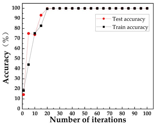
Figure 8.
Fault diagnosis accuracy of CEEMDANICA-TDCNN.
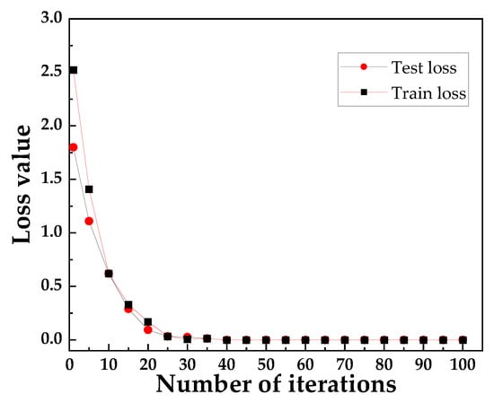
Figure 9.
The variation trend of loss value for CEEMDANICA-TDCNN.
It can be seen from Figure 8 that after 18 iterations, the training accuracy and testing accuracy of the model reached more than 95%. When the number of iterations reached 20, the training and testing accuracy were all 100%. Although the original signal was mixed with noise with a low signal-to-noise ratio, the method adopted could still accurately extract effective feature information from the rolling-element bearing vibration signals with different fault modes, and could identify different fault types quickly and with a high accuracy.
According to the trend change in the loss value of the model, the loss value maintains a stable decline with the increase in the number of iterations, and finally approaches 0. Moreover, the loss value of the model has no obvious repetition in the training and testing process, which indicates that the model has good robustness.
The results of several groups of experiments showed that the bearing fault identification model adopted in this paper could be applied to the pattern recognition of rolling-element bearings with different fault types under continuous variable speed conditions, and an excellent classification effect was achieved. The classification confusion matrix is shown in the Figure 10.
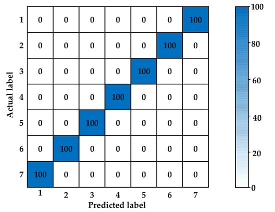
Figure 10.
Classification confusion matrix of CEEMDANICA-TDCNN.
4.3. Comparison of Results
Besides CNN, there were other deep learning models in the current classification model. In order to compare the classification results of different models, the feature data preprocessed by CEEMDANICA were inputted to the stacked autoencoder (SAE), back propagation neural network (BPNN) and multilayer perceptron (MLP) models.
The specific parameter settings of each model were as follows: SAE: architecture parameters were 1600–500−500–7. The learning rate, momentum and sparsity parameters were set to 0.1, 0.9 and 0, respectively. The number of training and testing iterations was 100. BP neural network: its structure was 1600–6−6–7, and the learning rate, momentum and iteration times were 0.001, 0.9 and 100, respectively. The number of neurons in each layer of MLP was 1000, its activation function was ReLU, and the number of iterations was 100. The ratio of training sample size to test sample size of all models was 4:1, and 100 iterations were performed. In order to ensure the iterative stability of each model and to eliminate accidental phenomena, each model was trained and tested for 10 times, and the average value was taken. The fault identification results of different models are shown in Table 4 and Figure 11.
Table 4.
Recognition results of different deep learning models.
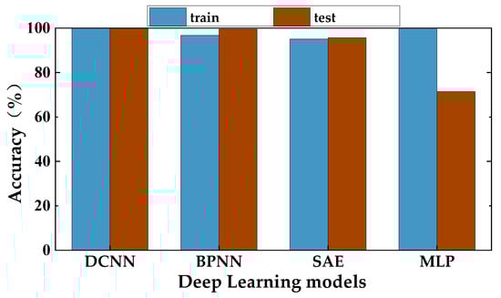
Figure 11.
Classification confusion matrix of CEEMDANICA-TDCNN.
According to the recognition results in Table 4, when the input characteristic matrix of the same size was used, the training accuracy and test accuracy of the TDCNN model selected in this paper could reach 100%, and the target could be reached after only 18 iterations. The actual iteration time was 24 s, which is far less than the iteration time of other models.
Among other models, BPNN and SAE have also achieved high recognition accuracies, but took a long time. Their classification accuracy was found to fluctuate in the process of adjacent experiments, and the stability of the model needs improving; the test accuracy of the MLP model was low, less than 80%, and its classification results were related to the number of training sets and test sets. When the data sets were small, the classification results of the model were not ideal and the classification accuracy was not high enough, indicating that the applicable conditions of the model had certain limitations.
It can be seen from Figure 11 that compared with other models, the model of CEEMDANICA combined with TDCNN had a strong feature learning ability, a good classification effect and fewer iterations were required for the single fault, composite fault, severe fault and slight fault of the automatic transmission rolling-element bearings.
5. Conclusions
By using CEEMDANICA to decompose the original vibration signal, the problem of mode aliasing is greatly improved, and the fault feature information can be extracted effectively. Through multiscale permutation entropy, box dimension, correlation coefficient and kurtosis index, ICA components are effectively filtered, and redundant noise is filtered.
A two-dimensional convolutional neural network model was constructed. By setting the model architecture and super parameters reasonably, it had a higher learning efficiency than other deep learning models.
The combination of CEEMDANICA and TDCNN extracted the characteristic components using the comprehensive index method. A transmission rolling-element bearing fault test platform was established, and the fault diagnosis of different degrees of fault, single fault and compound fault, was realized. This is of great significance to the condition monitoring and operation and maintenance of automatic transmissions.
Author Contributions
Conceptualization, G.L. and Y.C.; methodology, G.L. and W.W.; software, W.W.; validation, G.L. and Y.C.; formal analysis, W.W and R.L.; investigation, G.L.; resources, Y.C. and Y.W.; data curation, G.L.; writing—original draft preparation, G.L.; writing—review and editing, G.L.; visualization, Y.C.; supervision, Y.C.; project administration, Y.W.; funding acquisition, Y.W. All authors have read and agreed to the published version of the manuscript.
Funding
This research was funded by the National Key R&D Program of China (NO. 2018YFE0207000).
Data Availability Statement
Not applicable.
Conflicts of Interest
Wenqing Wang is an employee of Weichai Power Co., Ltd. The paper reflects the views of the scientists, and not the company.
References
- Ranjan, R.; Ghosh, S.K.; Kumar, M. Fault diagnosis of journal bearing in a hydropower plant using wear debris, vibration and temperature analysis: A case study. Proc. Inst. Mech. Eng. 2020, 234, 235–242. [Google Scholar] [CrossRef]
- Sharma, R.B.; Parey, A. Condition monitoring of gearbox using experimental investigation of acoustic emission technique. Procedia Eng. 2017, 173, 1575–1579. [Google Scholar] [CrossRef]
- Guan, Y.C.; Tong, P.; Feng, Z.P. Analysis of fault current signal characteristics of planetary gearbox based on ICEEMDAN method and frequency demodulation. Vib. Shock 2019, 38, 41–47. [Google Scholar]
- Zhang, X.X.; Li, S.B.; Zhe, L.X. Research on fault diagnosis of rolling bearing based on machine learning algorithm. Comb. Mach. Tools Autom. Process. Technol. 2020, 7, 36–39+44. [Google Scholar]
- Wang, J.; Du, G.; Zhu, Z. Fault diagnosis of rotating machines based on the EMD manifold. Mech. Syst. Signal Process. 2020, 135, 106443. [Google Scholar] [CrossRef]
- Long, J.Y.; Qin, Y.X.; Yang, Z. Discriminative feature learning using a multiscale convolutional capsule network from attitude data for fault diagnosis of industrial robots. Mech. Syst. Signal Process. 2023, 182, 109569. [Google Scholar] [CrossRef]
- Wang, H.; Dong, G.M.; Chen, J. A novel dictionary learning named deep and shared dictionary learning for fault diagnosis. Mech. Syst. Signal Process. 2023, 182, 109570. [Google Scholar] [CrossRef]
- Zhou, K.; Diehl, E.; Tang, J. Deep convolutional generative adversarial network with semi-supervised learning enabled physics elucidation for extended gear fault diagnosis under data limitations. Mech. Syst. Signal Process. 2023, 185, 109772. [Google Scholar] [CrossRef]
- Zinai, R.; Hammami, A.; Chaari, F. Gear fault diagnosis under non-stationary operating mode based on EMD, TKEO, and Shock Detector. C. R. Mec. 2019, 34, 663–675. [Google Scholar] [CrossRef]
- Ge, J.; Niu, T.; Xu, D. A rolling bearing fault diagnosis method based on EEMD-WSST signal reconstruction and multi-scale entropy. Entropy 2020, 22, 290. [Google Scholar] [CrossRef] [PubMed]
- Hou, J.; Wu, Y.; Gong, H. A novel intelligent method for bearing fault diagnosis based on EEMD permutation entropy and gg clustering. Appl. Sci. 2020, 10, 386. [Google Scholar] [CrossRef]
- Lobato, T.H.G.; Silva, R.R.D.; Costa, E.S.D. An integrated approach to rotating machinery fault diagnosis using, EEMD, SVM, and augmented data. J. Vib. Eng. Technol. 2020, 8, 403–408. [Google Scholar] [CrossRef]
- Li, G.H.; Fu, Z.F.; Zeng, X. Rolling bearing fault diagnosis based on EEMD and SOM. Noise Vib. Control 2020, 40, 87–91. [Google Scholar]
- Xiao, M.; Zhang, C.; Wen, K. Bearing fault feature extraction method based on complete ensemble empirical mode decomposition with adaptive noise. J. Vibroeng. 2018, 20, 2622–2631. [Google Scholar] [CrossRef]
- Vanraj Dhami, S.S. Non-contact incipient fault diagnosis method of fixed-axis gearbox based on CEEMDAN. R. Soc. Open Sci. 2017, 4, 170616. [Google Scholar] [CrossRef] [PubMed]
- Huang, C.; Lin, J.; Ding, J. A novel wheelset bearing fault diagnosis method integrated CEEMDAN, periodic segment matrix, and SVD. Shock Vib. 2018, 2018, 1382726. [Google Scholar] [CrossRef]
- Lei, Y.; Liu, Z.; Ouazri, J. A fault diagnosis method of rolling element bearings based on CEEMDAN. Proc. Inst. Mech. Eng. Part C: J. Mech. Eng. Sci. 2017, 231, 1804–1815. [Google Scholar] [CrossRef]
- Hu, C.; Shen, B.G.; Xie, Z.M. Fault diagnosis method of bearing based on EMD-FastICA and DGA-ELM network. Sol. Energy J. 2021, 42, 208–219. [Google Scholar]
- Lu, Q.; Li, M. A method combining fractal analysis and single channel ICA for vibration noise reduction. Shock Vib. 2021, 2, 1–10. [Google Scholar] [CrossRef]
- Song, Y.Z.; Tang, B.P.; Yan, B.S. Bearing fault diagnosis method based on EWT and ICA combined noise reduction. Comb. Mach. Tools Autom. Process. Technol. 2020, 7, 45–48, 54. [Google Scholar]
Publisher’s Note: MDPI stays neutral with regard to jurisdictional claims in published maps and institutional affiliations. |
© 2022 by the authors. Licensee MDPI, Basel, Switzerland. This article is an open access article distributed under the terms and conditions of the Creative Commons Attribution (CC BY) license (https://creativecommons.org/licenses/by/4.0/).