Path-Planning Strategy for Lane Changing Based on Adaptive-Grid Risk-Fields of Autonomous Vehicles

Abstract

The quantification and effective representation of safety risks for scenarios in structured road traffic environments of autonomous driving are currently being investigated in an active way. Based on artificial potential fields, a risk-field model for the traffic environment that considers the motion state of an obstacle vehicle is established, and an adaptive-grid risk-field method is proposed for autonomous vehicles. In this method, the traffic environment is meshed initially, and adaptive-grid division is performed using a quadtree grid-dividing strategy for root grids where the grid risk values are within the division interval, which allows for a more accurate quantification of traffic environment risk values. Adding adaptive-grid risk-field parameters to the cost function of the path-planning algorithm improves the accuracy of path safety risk assessment and completes the evaluation and selection of the optimal lane-change path. Simulation results show that the adaptive-grid risk-field established in this paper can effectively express the safety risks of the traffic environment, and the path-planning algorithm incorporating the adaptive-grid risk-field can obtain better paths for lane change compared with the traditional path-planning algorithm, while ensuring the safety of lane change.

1. Introduction

In the 21st century, with the development of intelligent network technology, autonomous driving technology has become a hot research topic. Lane change path planning plays a very important role in autonomous driving systems. Lane change path planning can get a desired driving path from the current lane to the target lane under certain constraints based on the real-time environment model.

Traditional lane-changing path planning algorithms rely on collision detection algorithms based on obstacle geometric boundaries when evaluating path safety, thus failing to take into account the safety risks around obstacles. However, the safety risk around obstacles cannot be ignored. For example, the safety risk around an obstacle for a vehicle running at a higher speed is greater than that for a vehicle running at a lower speed; the closer to the obstacle or to the road boundary, the higher the safety risk for the vehicle. Therefore, in this paper, we use the idea of potential field to establish the safety risk models of obstacle cars, road boundaries and road dividers in structured roads, so as to obtain the traffic environment risk-field model as the basis for the evaluation of path safety in path-planning algorithm.

Although research on risk-fields in traffic environments has been conducted for many years, the application of risk-field models to lane-change path planning algorithms, however, still has some problems:

• The existing risk-field models are all continuous models, which are difficult to apply in spatially continuous traffic environments.
• In addition, most of the existing risk-field models do not consider the motion state of the obstacle vehicle.

In this study, we propose a lane-change path planning method based on adaptive-grid risk-field. The method establishes a risk-field model of the traffic environment considering the motion state of obstacle vehicles. The quadtree grid-dividing method and the risk-field model are combined to perform adaptive-grid risk representation of the traffic environment so as to obtain a discrete traffic environment risk-field with high accuracy, and the risk-field is applied to the autonomous vehicle lane-changing path-planning algorithm to provide traffic environment safety information for path safety assessment, so as to plan a desired path with higher safety.

The remainder of the paper is organized as follows: In Section 3 and Section 4, an adaptive-grid risk-field model is introduced. Based on a traffic environment risk-field model, the quadtree grid division method is used to divide the root grid that satisfies the dividing rule. Section 5 presents a path-planning method based on dynamic programming, and path risk terms are introduced in the cost function. In Section 6, a verification of the proposed method is presented based on several typical scenarios using the typical MATLAB/CarSim co-simulation platform. Section 7 summarizes the contents of this study.

2. Related Works

In the decision-making process for autonomous driving systems, traffic environment safety risk models can provide important environmental safety risk information at the decision-making level. Some scholars have established risk-field models for traffic environments based on potential fields.

At the end of the 20th century, Khatib [1] first proposed an artificial potential field path-planning algorithm. Henceforth, the planning and control of robots or autonomous vehicles based on artificial potential fields has received widespread attention [2,3,4]. Owing to the development of autonomous driving and intelligent transportation, scholars have extensively used potential field theory to assess safety risks in the traffic environment. Wolf et al. [5] established a highway potential-field function to assist autonomous vehicle obstacle avoidance by expressing the potential vehicle field as a wedge and considering the velocity potential when constructing the potential field. Wang et al. [6] proposed a new concept of the driving risk-field; they established a kinetic field determined by a moving object, a potential field determined by the road environment, and a behavioral field determined by the characteristics of the driver. Qiang et al. [7] proposed a lateral planning method based on the potential field, which establishes a potential field model based on the characteristics of traffic participants and traffic rules and used the potential field information to plan the travel path. Rasekhipour et al. [8] established potential functions for obstacles and roads, which were integrated into the objective function in a path planner based on model prediction. Li et al. [9] established a safety potential field in an intelligent networked environment; additionally, they established a vehicle-following model based on a safety potential-field model by calibrating the safety potential-field model using 412 groups of NGSIM (next generation simulation) following data. Li et al. [10] proposed a dynamic control authority-allocation strategy based on an elliptical driving safety-field to solve the human–machine problem in the obstacle avoidance process. Zhu et al. [11] established a personalized path-changing trigger model based on lane-changing data of actual drivers and artificial potential field theory. Tian et al. [12] introduced the collision time, vehicle physical attributes, motion states, and heading angles into a risk-field model to improve its accuracy. Jia et al. [13] established a unified vehicle potential field function based on the Lennard–Jones potential and applied the safety potential field to the following behavior of CAV; the model still has a smoother response curve. Cheng et al. [14] established a traffic environment complexity evaluation model using potential field theory, which integrates the physical attributes and state parameters of environmental elements to reduce the environmental complexity evaluation errors.

However, the risk-field model is difficult to apply directly to the traffic environment in a continuous space, whereas the grid map can discretize the continuous space, thus allowing the risk-field model to be applied to autonomous vehicle systems. Environmental gridding methods have been widely used [15,16,17,18]; however, an environment representation based on a uniform grid size cannot accurately represent a complex environment. This problem can be solved using the adaptive-grid approach.

Fairfield [19] proposed an efficient octree spatial management method that can dynamically adjust the number of particles and improve the accuracy of modelling large environments. Li et al. [20] proposed a variable-resolution occupancy grid map based on a quadtree structure, where the nodes in the quadtree structure were merged or divided to adapt the grid resolution to the actual environment, thereby achieving a grid map with improved accuracy. Jin [21] proposed an online adaptive-resolution terrain mapping method based on the fusion of Gaussian processes to improve the environmental representation of UAVs, which can adaptively adjust the resolution of terrain mapping based on environmental changes and improve the quality of real-time environmental information acquisition. Vespa et al. [22] dynamically selected an appropriate grid size based on the octree structure and sensor data, and experimental results showed that this method significantly improved the quality of grid maps compared with a fixed-resolution grid. Chen et al. [23] proposed a probabilistic quadtree map that eliminates the uncertainty of the local environment representation and enables the efficient and high-quality representation of large two-dimensional environments.

Scholars have extensive investigated risk-fields from previous studies. However, the proposed risk-field models are difficult to apply in spatially continuous traffic environments, thus making it difficult to provide safety risk information of traffic environments based on risk-field models for decision making and planning. The application of the risk- field model on the basis of the grid traffic environment can make the continuous risk-field model discrete, thus solving the problem that the continuous risk-field model is difficult to be applied to the spatially continuous traffic environment. However, if the traffic environment is divided into a fixed grid size, the accuracy of the traffic environment risk representation cannot be guaranteed. Therefore, an adaptive-grid risk-field method for autonomous vehicles is proposed herein. Based on the initial gridding of the traffic environment, a quadtree grid division method was used to establish an adaptive-grid traffic environment risk-field, where the number of regional grids changes in real time with the risk value, which improves the applicability of the risk-field model and the accuracy of the traffic environment risk expression. Risk-field information was integrated into the cost function for route-change planning to improve the accuracy of route safety-risk evaluation.

3. Risk-Field Modeling for Traffic Environments

In a structured road traffic environment, the main constraints during the driving of vehicles are the road dividing line, road boundary, and obstacle vehicle. Because the traffic environment is highly uncertain, expressing the constraints above via a state process would result in an extremely complex process of constraint expression, whereas expressing the constraints in the traffic environment in a unified form for the traffic environment risk-field simplifies the constraint expression. The risk-field established in this study differs from that of the typical vector field. The risk-field generated by each factor will not cancel but will form the total risk-field by superimposing each other. In a risk-field, the risk value is proportional to the safety risk.

3.1. Road Divider Risk-Field

In a structured road traffic environment, road dividers are soft constraints used to delineate lanes, constrain vehicles such that they traverse in an orderly manner within lanes, and allow vehicle lane changes. The divider risk-field was modeled based on the divider characteristics above:

$$Z_S={\displaystyle \sum _{n=1}^2{A}_S\exp \left(-\frac{{\left(y-y_{\mathrm{sn}}\right)}^2}{2{\sigma }_S{}^2}\right)}$$

(1)

where $Z_S$ is the road divider risk value; $A_S$ is the peak of the divider risk-field; $y_{\mathrm{sn}}$ is the lateral position of the nth road divider of the road; ${\sigma }_S$ is the shape parameter of the road divider risk-field, which determines the gradient norm of the divider risk-field.

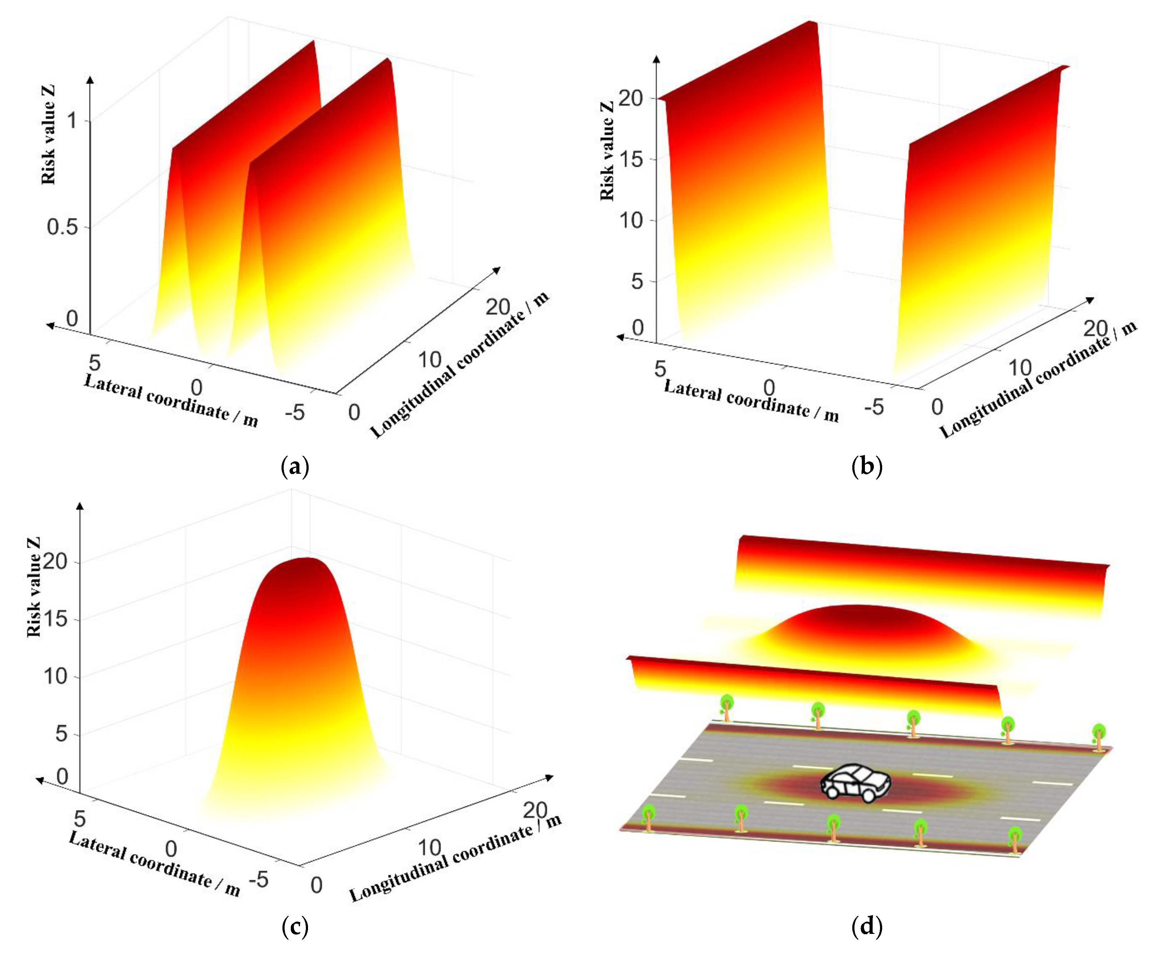
Based on the characteristics of the road-divider constraints, $A_S=1$ and ${\sigma }_S=0.5$ are set to establish the risk-field of the road divider, as shown in Figure 1a. As shown, the risk-field of the road divider expands to both sides with the dividing line as the center line, and the ranges of the risk-field and peak are small. Meanwhile, the gradient norm of the risk-field is large.

3.2. Road Boundary Risk-Field

In a structured road traffic environment, the road boundary is a difficult constraint that restricts a vehicle from driving within the road range. The risk-field of the road boundary was modeled based on the characteristics of the road boundary:

$$Z_{\mathrm{B}}={\displaystyle \sum _{n=1}^2{A}_B}\exp \left(-\frac{{\left(y-y_{b_n}\right)}^2}{0.8{\sigma }_B^{}{}^2}\right)$$

(2)

where $Z_{\mathrm{B}}$ is the road boundary risk value; $A_B$ is the peak value of the road boundary risk-field; $y_{b_n}$ is the lateral position of the nth road boundary of the road; ${\sigma }_B^{}$ is the shape parameter of the road boundary risk-field, which determines the risk-field gradient norm of the road boundary risk-field.

Based on the characteristics of the road boundary constraint, $A_B=20$ and ${\sigma }_B^{}=1$ are set to establish the road boundary risk-field, as shown in Figure 1b. When approaching the road boundary, the road boundary risk value increases rapidly, and the risk-field range is small.

3.3. Obstacle Vehicle Risk-Field

Obstacle vehicles are the leading participants in traffic environments and the main cause of traffic accidents. Their movement characteristics significant affect the safety risk in a traffic environment. Because the longitudinal velocity norm of an obstacle vehicle is much greater than the lateral velocity norm, the effect of the obstacle vehicle on the safety of vehicles in the same lane is much greater than that of vehicles in the side lane. Based on the characteristics of the obstacle vehicle above, the risk-field of an obstacle vehicle was modeled:

$$Z_V={\displaystyle \sum _{\mathrm{n}=1}^p{A}_V\exp \left(-{\left(\frac{{\left(\left(x-x_n\right)/e\right)}^2}{2{\sigma }_x^2}+\frac{{\left(y-y_n\right)}^2}{2{\sigma }_{\mathrm{y}}^2}\right)}^2\right)}$$

(3)

$$e=M_i\times \{\begin{array}{ll}\exp \left(-\left|x-x_n\right|\right)+c+a,\hfill & a>0\wedge x⩾x_n\hfill \\ \left(\exp \left(-\left|x-x_n\right|\right)+1\right)/5,\hfill & a>0\wedge x<x_n\hfill \\ \left(\exp \left(-\left|x-x_n\right|\right)+1\right)/5,\hfill & a<0\wedge x⩾x_n\hfill \\ \exp \left(-\left|x-x_n\right|\right)+c+\left|a\right|,\hfill & a<0\wedge x<x_n\hfill \\ 1\hfill & a=0\hfill \end{array}$$

(4)

$$M_n={\mathrm{m}}_n\cdot \left(1.566\times {10}^{-14}\cdot {\mathrm{v}}_n{}^{6.687}+0.3345\right)$$

(5)

where $Z_V$ is the risk value of the obstacle vehicle; $A_V$ is the peak value of the obstacle vehicle risk-field; $(x_n,y_n)$ is the coordinate of the nth obstacle vehicle; ${\sigma }_x^{}$ and ${\sigma }_y^{}$ are the shape parameters of the obstacle vehicle risk-field, which determine the gradient norm of the obstacle vehicle risk-field in the lateral and longitudinal directions, respectively; $e$ is the motion factor that characterizes the effects of the speed, acceleration, and mass of the obstacle vehicle on the obstacle vehicle risk-field; $M_n$ is the equivalent mass of the nth obstacle vehicle. Some researchers [6,24] assumed that the equivalent mass of a vehicle is related to its speed and actual mass and, based on an accident sample set, established the form of the equivalent mass, as shown in Equation (5).

Based on the characteristics of the obstacle vehicle, $A_V=20$, ${\sigma }_x^{}=1.25$, and ${\sigma }_y^{}=0.8$ were set to establish the risk-field of the obstacle vehicle, as shown in Figure 1c. As shown, the risk-field of the obstacle vehicle is oval, i.e., compared with the side lane, the risk-field of the obstacle vehicle features a more extensive distribution range in the lane where the obstacle vehicle is located. The obstacle vehicle’s risk peak is large, and the field range is more extensive. Moreover, the gradient norm of the risk-field is small.

The motion factor $e$ is introduced into the risk-field of obstacle vehicles to match the range of the risk-field of obstacle vehicles with the motion state. Figure 2 shows the effect of the motion state of the obstacle vehicles on the risk-field distribution. Among them, $V{E}_a$, $V{E}_b$, $V{E}_c$, and $V{E}_e$ are equal in quality, and the quality of $V{E}_d$ is twice that of $V{E}_a$.

By comparing the risk-field distributions of vehicles $V{E}_a$, $V{E}_b$, $V{E}_c$, it is shown that because the acceleration of $V{E}_b$ is greater than 0, compared with the risk-field range of $V{E}_a$, the risk-field range behind $V{E}_b$ is smaller, whereas the risk-field range in front is larger. Because the acceleration of $V{E}_c$ is less than 0, compared with the risk-field range of $V{E}_a$, the risk-field range in front of $V{E}_c$ is smaller, and the risk-field range in the back is larger. By comparing the risk-fields of cars $V{E}_a$, $V{E}_d$, and $V{E}_e$, it is shown that because cars $V{E}_d$ and $V{E}_a$ have the same speed, but the mass of $V{E}_d$ is twice that of $V{E}_a$, the risk-field distribution of $V{E}_a$ is larger than that of $V{E}_d$. Because the velocity of $V{E}_e$ is one-half that of $V{E}_a$, the distribution of $V{E}_e$’s risk-field is smaller than the risk-field range of $V{E}_a$.

3.4. Total Risk-Field Establishment

The total environmental risk-field for traffic was obtained by superimposing the risk-fields above, as shown in Figure 1d.

$$Z\left(x,y\right)=Z_S\left(x,y\right)+Z_B\left(x,y\right)+Z_V\left(x,y\right)$$

(6)

4. Adaptive-Grid Risk-Field Modeling

The traffic environment risk-field was established as described above. However, the actual traffic environment is a continuous space, and the risk-field model is a continuous model that is difficult to solve and is directly applied to an autonomous vehicle system. Therefore, to improve the applicability and accuracy of the risk-field theory, an adaptive-grid risk-field method is proposed herein.

4.1. Initial Gridding

To apply risk-field theory to a grid map, an initial grid of the traffic environment must be created, and the unit grid size in the initial grid map must be determined.

In the case of a traffic environment with a fixed size, when the complexity of traffic environment C is larger, more accurate environmental information is required to ensure the accuracy of the environmental expression. Thus, the more the number of grids in the traffic environment, the smaller is the unit grid area $d_r{}^2$, i.e., $C\propto \frac{1}{d_r^2}$.

The edge length of the initialized grid is expressed as follows:

$$dr=\sqrt{\frac{k_r}{C}}$$

(7)

where $k_r$ is the proportional coefficient between the environmental complexity and the square of the grid side length.

In a structured road traffic environment, the higher the quantity and variety of obstacle vehicles, the greater is the difference between the moving status of the cars, and the higher is the complexity level in the traffic environment. Furthermore, the greater the road curvature, the greater are the steering angle and steering angular velocity of the obstacle vehicle in the traffic environment; consequently, the motion state of the obstacle vehicle becomes more unstable, and the complexity of the traffic environment increases. Therefore, the complexity of the traffic environment is primarily affected by the complexity of the obstacle vehicle and road. Based on the characteristics above, a formula for calculating the complexity of a traffic environment is established as follows:

$$\begin{array}{cc}C\text{=}\hfill & w_1\left({\sum }_{n=1}^p\left({\text{Ω}}_1{M}_n\text{+}{\Omega }_2{a}_n\right)\right)\text{+}{w}_2\cdot \overline{K}\hfill \\ ==\hfill & w_1({\sum }_{r=1}^p({\text{Ω}}_1\left({\text{m}}_n\cdot \left(1.566\times {10}^{-14}\cdot {\text{v}}_n{}^{6.687}+0.3345\right)\right){\text{+}\Omega }_2{a}_n\left)\right)\text{+}{w}_2\cdot \overline{K}\hfill \end{array}$$

(8)

where $w_1$ and $w_2$ are the complexity weight coefficients of the obstacle vehicle and road, respectively; ${\mathsf{\Omega }}_1$ and ${\mathsf{\Omega }}_2$ are the equivalent mass weight coefficient and acceleration weight coefficient of obstacle vehicle, respectively; $a_n$ is the acceleration of the nth obstacle vehicle; $\overline{K}$ is the mean value of the lane line curvature within the grid map.

4.2. Triggering Rule of Grid Division

After the initial gridding of the traffic environment, the initial grid was defined as the root grid. The grid-coverage areas with high- and low-risk values can be considered absolutely dangerous or absolutely safe, respectively; therefore, these grids need not be divided. For the remaining grid, the areas covered by the grid feature different risk levels, i.e., some areas are associated with a high security risk, whereas others are associated with a low security risk. To ensure the accuracy of the risk-field, this section of the grid must be divided. Therefore, the following grid-dividing trigger rules, as listed in

Table 1. Triggering rule of grid division.

Range of Value at Risk	Name	Situation of Division
(−∞, L)	Low risk grid	No
(L, H)	Medium risk grid	Yes
(H, +∞)	High risk grid	No

, were formulated.

4.3. Grid-Division Method

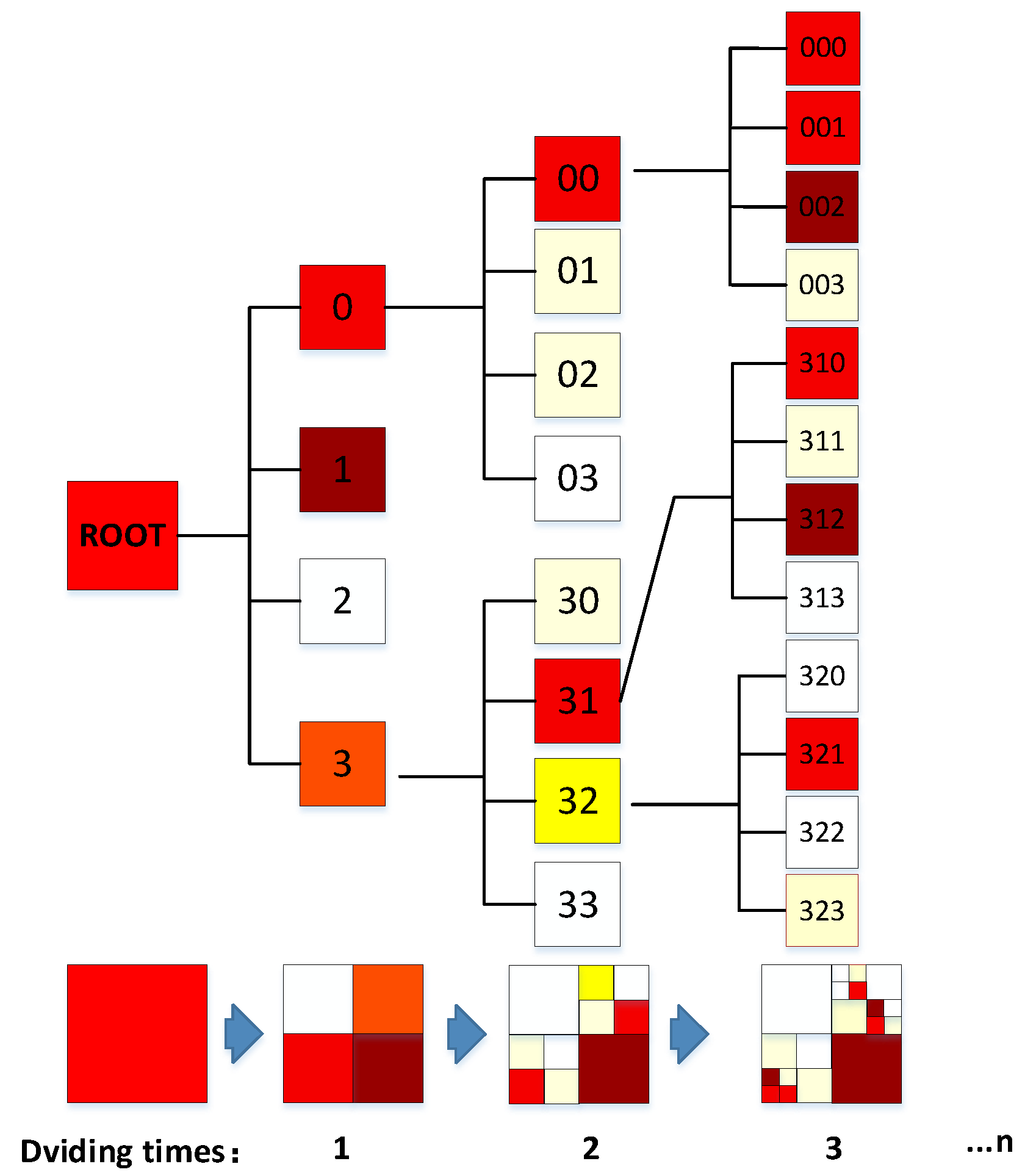
When a grid is divided, the coordinates of the resulting subgrids must be determined. In this regard, we adopted the quadtree grid-dividing method, and grid numbering rules were designed based on the grid numbering. Subsequently, the center coordinates of the subgrids could be calculated.

Figure 3 shows a division sample of the root grid. This root grid conforms to the grid-division trigger rules; first, it is divided into subgrids numbered 0, 1, 2, and 3 (which denote subgrids in the lower left, lower right, upper left, and upper right, respectively). Among these subgrids, subgrids 0 and 3 conform to the grid-division trigger rules. Therefore, these subgrids must be divided. Grid 3, for example, was divided into grids 30, 31, 32, and 33. Grid 31 was further divided into grids 310, 310, 311, 312, and 313. Therefore, the number of subgrids can be expressed as X1, X2, ..., Xn, where Xi can be 0, 1, 2, or 3. The center coordinate of a subgrid after the division can be expressed as:

$$x_c=x_f+{\left(-1\right)}^{\lambda }\frac{d_f}{4}$$

(9)

$$y_c=y_f+{\left(-1\right)}^u\frac{d_f}{4}$$

(10)

The side length of the subgrid is expressed as:

$$d_c\text{=}{d}_f\text{/}2$$

(11)

where $\left(x_f,y_f\right)$ is the center coordinate of the parent grid, and $d_f$ is the width of the parent grid. The values of $\lambda$ and $u$ are listed in

Table 2. Values of $\lambda$ and $u$.

Xn	$\mathit{\lambda }$	$\mathit{u}$
0	1	1
1	2	1
2	1	2
3	2	2

.

4.4. Adaptive Dividing Risk-Field

Figure 4 shows the flowchart for establishing the adaptive-grid risk-field. After obtaining information regarding the obstacle cars and roads in the environment, the size of the root grid is calculated, and the risk value of the center point of each root grid is detected. If the root grid conforms to the triggering rule of grid division and the grid size is greater than $d_{\min }$, then the grid is divided; otherwise, the division is completed, and the risk value is calculated for each subgrid. If the root grid conforms to the triggering rule of grid division and the grid size is greater than $d_{\min }$, then the grid is divided; otherwise, the division is completed. By repeating the cycle above, the center coordinates of each grid after grid division can be obtained using Equations (9) and (10).

Substituting Equations (9) and (10) into Equation (6), the risk value of a grid after division is obtained as follows:

$$\begin{array}{l}Z\left(x,y\right)=Z_S\left(x,y\right)+Z_B\left(x,y\right)+Z_V\left(x,y\right)\\ ={\sum }_{n=1}^2{A}_s\exp \left(-{\left(y_f+{(-1)}^u\frac{d_f}{4}-y_{sh}\right)}^2/2b_s^2\right)\\ +{\sum }_{n=1}^2{A}_B\exp \left(-{\left(y_f+{(-1)}^u\frac{d_f}{4}-y_{b_n}\right)}^2/0.8{\sigma }_B^2\right)\\ +{\sum }_{\mathrm{n}=1}^p{A}_V\exp \left(-{\left({\left(\left(x_f+{(-1)}^{\lambda }\frac{d_f}{4}-x_n\right)/e\right)}^2/2{\sigma }_x^2+{\left(y_f+{(-1)}^u\frac{d_f}{4}-y_n\right)}^2/2{\sigma }_y^2\right)}^2\right)\end{array}$$

(12)

Finally, the risk values of all grids after division are calculated, and the risk values of each grid are mapped to the grid map to generate an adaptive-grid risk-field, as shown in Figure 5.

In the ROOT layer (see Figure 5), the root grid edge length is $dr$, ROOT0 and ROOT1 are high-risk grids that are not divided, ROOT2 and ROOT3 are medium-risk grids that are divided. In the Level1 layer, ROOT2 is divided into ID0, ID1, ID2, and ID3, and the length of the subgrid of ROOT2 is $d_2=d_r/2$. ID0 is a non-divided high-risk grid. ID1, ID2, and ID3 are medium-risk grids that continue to be divided. Regarding ID2, based on the grid-dividing theory presented in Section 3.2, $\lambda =1$, $u=2$, and $Z\left(\mathrm{ID}2\right)=Z\left(x_r-d_r/4,x_r+d_r/4\right)$. In the Level2 layer, ID2 is divided into ID20, ID21, ID22, and ID23; the edge length of subgrid ID2 is $d_3=d_2/2$. ID21, ID22, and ID23 are non-divided low-risk grids; ID20 is a non-divided medium-risk grid, but $d_3<d_{min}$; thus, ROOT2 is not divided. For ID21, based on the grid-dividing theory presented in Section 3.2, $\mu =1$, $\lambda =2$, and $Z\left(ID21\right)=Z\left(xr+dr/4,xr-dr/4\right)$. A comparison of the risk-field map of the ROOT layer and Level2 layer shows that the high- and low-risk root grids did not divide, whereas the medium-risk root grid was divided multiple times, and the area contained in the medium-risk grid was expressed precisely.

5. Optimal Lane-Change Path Selection Based on Discretized Risk-Field

5.1. Path Cluster Generation Based on Dynamic Programming

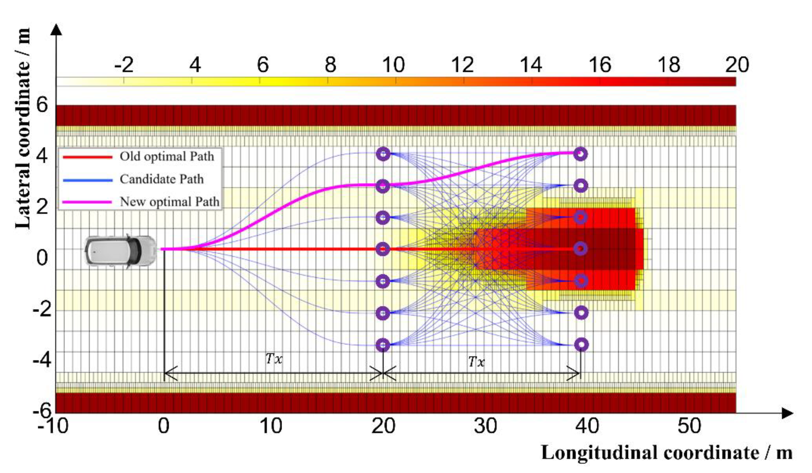
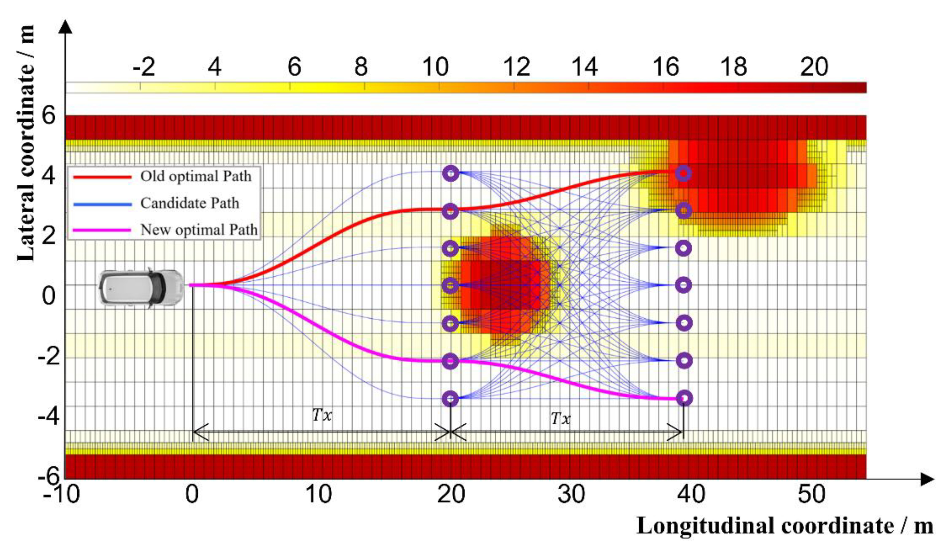
The shape of a structured road is regular; hence, sampling is a more suitable for generating a driving path on a structured road compared with other methods. As shown in Figure 6, seven sample points are defined in the direction perpendicular to the centerline, and two sampling layers with an interval $Tx$ of 20 m are defined in the direction parallel to the centerline of the road. The starting and sampling points in the path cluster are connected by polynomials. Because each layer contains multiple sampling points, a path cluster is generated using different combinations, and the results of this path cluster are reused in each period.

In structured roads, the lateral velocity and lateral acceleration of the vehicle at the start and end of the lane change process are often zero in order to ensure the comfort and safety of the vehicle during travel. In each layer of the path cluster, the starting and ending points of the path are obtained by sampling, so six boundary conditions must be considered in the process of generating each path: starting point position, ending point position, starting point lateral velocity, ending point lateral velocity, starting point lateral acceleration, and ending point lateral acceleration. The quintic polynomial has six unknown coefficients, which can satisfy the six boundary conditions in the path generation process. In addition, the second order derivative of the curvature of the path corresponds to the jerk of the circular motion of the steering wheel. Therefore, in order to make the second order derivative of the path curvature continuous, the polynomial used for the path must be a fifth order polynomial or higher, but the use of higher order polynomials will increase the risk of the Runge phenomenon appearing. Therefore, the path is planned using quintic polynomial:

$$y=k_0+k_{1}x+k_2{x}^2+k_3{x}^3+k_4{x}^4+k_5{x}^5$$

(13)

where $k_0\dots k_5$ are the coefficients of the quintic polynomial.

5.2. Path Selecting

Figure 6 shows the path-selection process. In the figure, the green paths are paths through the high-risk grid; the blue paths are the optional paths, and the red paths are the optimal paths. After the path cluster is obtained using the path-planning algorithm, optional paths are selected using the cost function, and an optimal path is obtained.

When the conventional cost function is used to evaluate the safety of the path, it only determines whether the path collides with the obstacle vehicle from the perspective of geometric space, i.e., it cannot consider the safety risk around the obstacle vehicle in the traffic environment. Hence, a path risk item was introduced into the cost function, and the risk information of the risk-field was used to evaluate the safety of the path.

Equation (14) expresses the cost function adopted in this study,

Table 3. Description of the parameters and evaluation terms in the cost function.

Cost Function Parameter	Meaning
$k$	Path point number of the i path
$u_1$	Expectation weight coefficient
$u_2$	Variance weight coefficient
$\cos t\left(k\right)$	Cost of the kth path point
$COST\left(\mathrm{i}\right)$	Cost of path(i)
$p_c\cdot a_c\left(k\right)$	Cost of path smoothness
$p_c$	Weight coefficient of path smoothness
$p_{\mathrm{d}}\cdot a_d\left(k\right)$	Cost of lateral distance to road centerline
$p_{\mathrm{d}}$	Weight coefficient of transverse distance to road centerline
$p_{\mathrm{s}}\cdot a_s\left(k\right)$	Path risk cost
$p_{\mathrm{s}}$	Path risk weight coefficient

describes the parameters and evaluation items in the cost function.

$$COST\left(\mathrm{i}\right)=u_{1}E(\cos t(k))+u_{2}D(\cos t(k))$$

(14)

$$\cos t\left(k\right)=p_c\cdot a_c\left(k\right)+p_d\cdot a_d\left(k\right)+p_s\cdot a_s\left(k\right)$$

(15)

$$a_c\left(k\right)=\mathrm{y}{\left(k\right)}^{{}^{\prime }2}+\mathrm{y}{\left(k\right)}^{{}^{″}2}$$

(16)

$$a_d\left(k\right)=\mathrm{d}{\left(k\right)}^2$$

(17)

$$a_s\left(k\right)=Z\left(k\right)$$

(18)

6. Algorithm Validation

The effectiveness of the proposed method was verified using the MATLAB/CarSim co-simulation platform and an actual vehicle test platform. Additionally, two typical lane-change scenarios were selected for adaptive-grid risk-field generation and path planning. In all scenarios, the road is a three-lane highway with a lane width of 3.75 m. In the path-generation section, the blue path is the candidate path planned by the path-planning algorithm; the red path is the optimal path selected by the conventional cost function, and the purple path is the optimal path selected by the cost function established in this study.

Table 4. Value of algorithm parameters.

Algorithm Parameter	Value	Algorithm Parameter	Value	Algorithm Parameter	Value
$L$	4	$A_V$	20	${\mathsf{\Omega }}_2$	1
$H$	12.5	${\sigma }_x$	1.25	$u_1$	1
$d_{\min }$	0.2 m	${\sigma }_y$	0.8	$u_2$	0.7
$A_S$	1	$k_r$	1.2	$p_c$	0.7
${\sigma }_S$	0.5	$w_1$	1	$p_d$	0.7
$A_B$	20	$w_2$	0.8	$p_s$	1
${\sigma }_B$	1	${\mathsf{\Omega }}_1$	1.2

shows the algorithm parameter values in the algorithm verification process.

6.1. Simulation Verification

Figure 7a shows a simulation scenario in which self-vehicle EGO1 traverses straight at a uniform speed of 60 km/h, and VE1 traverses straight at 60 km/h, with an acceleration of −0.6 m/s². The longitudinal distance between VE1 and EGO1 was 44 m. Figure 7b shows the idealized risk-field of the simulation scenario. The rear VE1 risk-field range is significantly larger than the front risk-field range because the acceleration of VE1 is less than 0.

Figure 7c shows the undivided-grid risk-field of the simulation scenario, whereas Figure 7d shows the adaptive-grid risk-field of the simulation scenario. The grid size shown in Figure 7c is fixed; therefore, the safety risk of the risk grid-coverage area cannot be accurately expressed. Figure 7d shows that in the middle-risk area, the number of grids is higher than those of other areas, and the risk expression is more refined, thus allowing the safety risk of the traffic environment to be expressed more accurately.

In Figure 8, because the longitudinal distance of the path cluster is less than the distance between VE1 and EGO1, the red path is defined as a non-collision path based on the conventional cost function; however, the cost function herein considers the security risks around VE1, and the risk value of the end region of the red path is high. Therefore, the cost function defines the red path as a high-risk path, and the purple path as the optimal path. Compared with the path selected by the conventional cost function, the path selected by the cost function established in this study is more secure.

In Figure 9a, the smoothness cost of the new path is greater than that of the traditional path, but the peak is less than 0.08. In Figure 9b, the cost of lateral offset between the new path and the road center line is obviously greater than that of the traditional path, but the peak value is less than 3.6, that is, the lateral offset between the new path and the road center line is always less than 1.9 m, and the cost of lateral offset between the new path and the road center line decreases rapidly to 0 after reaching the peak value. 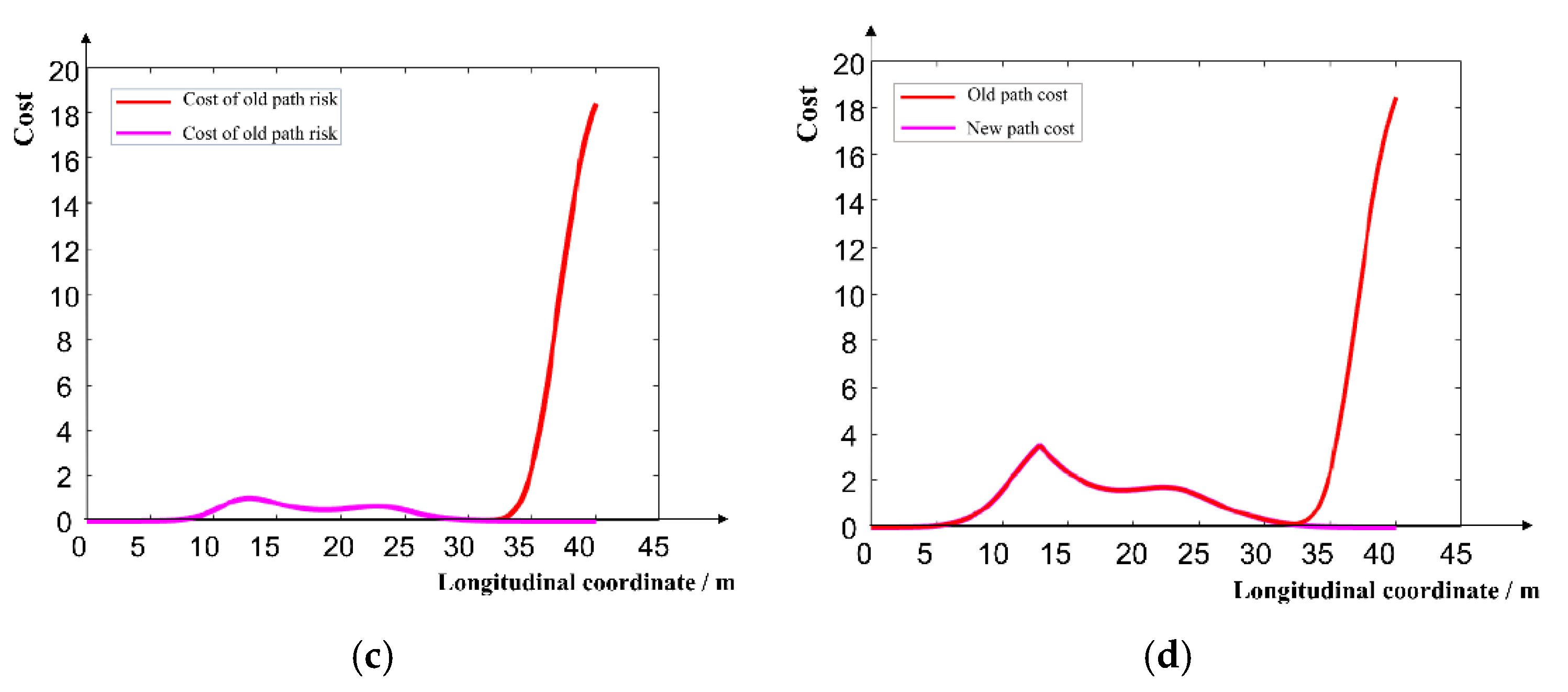In Figure 9c, the risk cost of the new path is always close to 0, while in the region with lateral displacement greater than 17 m, the risk cost of the traditional path increases rapidly and reaches a peak of 20, so the risk cost of the new path is obviously less than that of the traditional path. It can be seen from Figure 9d that the cost of the new path is obviously smaller than that of the traditional path. Through Equation (14), the comprehensive costs of the new path and the traditional path can be calculated as 1.2 and 47.4, respectively. Obviously, the cost of the new path is smaller. Therefore, compared with the traditional path, the new path has higher security under the premise that the cost of ride comfort and the cost of offset from the road center line meet the requirements.

6.2. Actual Vehicle Verification

As shown in Figure 10, in the actual vehicle verification section, an FAW Hongqi L3-class intelligent electric vehicle was used as self-vehicle EGO2. Details regarding the sensor configuration of EGO2 are listed in

Table 5. Hardware equipment of real vehicle test platform.

Serial Number	Equipment Name	Usage
(1)	dSPACE MicroAutoBoxII	1. Collecting and Preprocessing Related Sensor Data
		2. Implementation of lane changing algorithm and strategy; building algorithm model; calculating, storing, searching and outputting calculation results.
		3. Send the torque magnitude for longitudinal control, steering wheel angle signal for lateral control, etc., to the wire control chassis in the form of CAN telegrams
(2)	Millimeter wave radar ESR	Distance measuring sensors
(3)	Binocular camera	Visual mapping, semantic segmentation and lane line recognition, etc.
(4)	GPS positioning device SimPark982	Positioning output of vehicle latitude and longitude coordinates
(5)	Inertial navigation systems	Output of vehicle dynamics parameters
(6)	Chassis communication protocols	CAN telegram signal

.

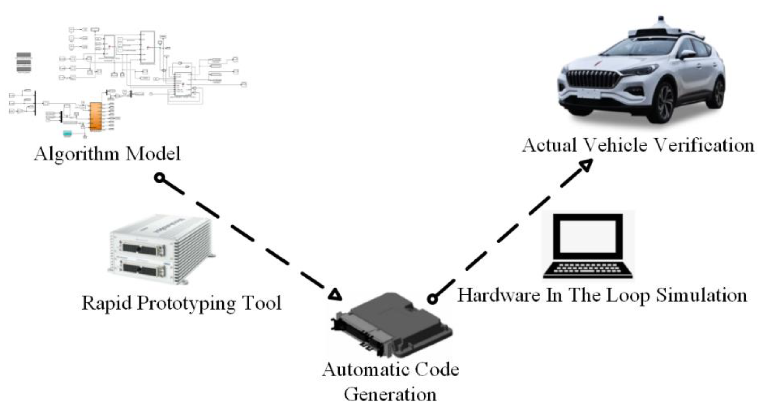
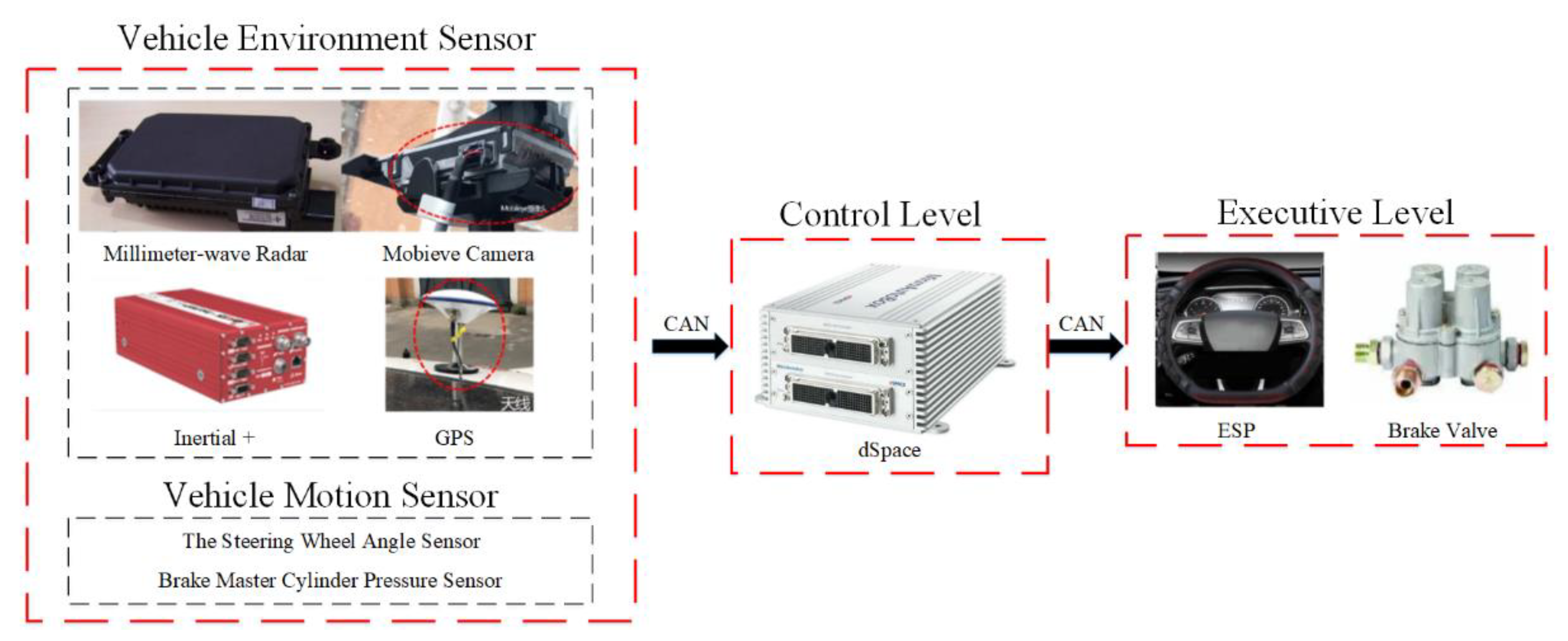
As shown in Figure 11, in order to quickly arrange the test scheme and facilitate rapid modification of the test, the test platform is built based on the dSpace rapid prototype test method, using rapid prototype automation tools and correctly setting the simulation parameters to achieve the purpose of quickly modifying the model optimization algorithm and to meet the needs of the actual vehicle verification. As shown in Figure 12, in the process of actual vehicle verification, dSpace obtains the sensor data through can, the algorithm in dSpace processes the sensor data and calculates the data of the control vehicle, and then the data of the control vehicle is passed to the actuator through CAN, so as to complete the verification of the algorithm.

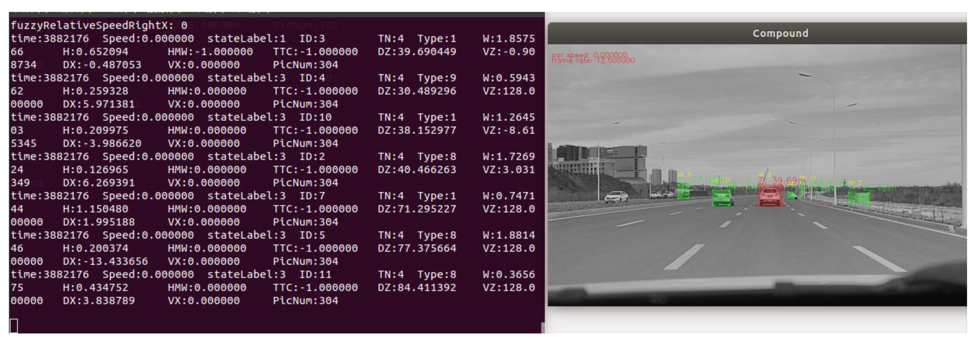
To better obtain information about the traffic environment, as shown in Figure 13. Semantic segmentation is used to detect vehicles and lane lines in the images captured by the camera to provide feature information of vehicles and lane lines for the gridded risk-field. For each pixel in the target image, the segmentation network of semantic segmentation assigns it to a certain set of pixel labels defined in advance. The method based on semantic segmentation realizes object classification by dividing the image into multiple regions and extracting the features of each region, so as to obtain the contour features of the front vehicle and the lane line. The VGG16 basic network is used as the pre-training network, and the SegNet network model is used to construct the scene segmentation network.

Figure 14 shows the test scenario for an actual vehicle in which self-vehicles EGO2 and VE2 are driven in a uniform straight line at a speed of 60 km/h, and VE3 is driven in a uniform straight line at a speed of 30 km/h. The longitudinal distance between VE2 and EGO2 was 44 m. The longitudinal distance between VE3 and EGO2 was 25 m.

Figure 15a is a schematic diagram of the actual vehicle scenario. Figure 15b shows the idealized risk-field of the actual vehicle scenario. The risk-field distribution range of VE3 was smaller than that of VE2 because the speed of VE3 was one-half that of VE2. Figure 15c shows the undivided grid risk-field of the simulation scenario, and Figure 15d shows the adaptive-grid risk-field of the simulation scenario, where the grid size in Figure 15c is fixed; therefore, the safety risk of the risk grid-coverage area cannot be accurately expressed. In the middle-risk area shown in Figure 15d, the number of grids is higher compared with those of other areas, and the risk expression is more refined, thus allowing the safety risk of the traffic environment to be expressed more accurately.

Because the longitudinal distance of the path cluster is less than the distance between VE2 and EGO2 (see Figure 16), the red path is defined as a non-collision path by the conventional cost. However, the cost function herein considers the security risks around VE2, and the risk value of the end region of the red path is large. Therefore, the cost function defines the red path as a high-risk path, and the purple path as the optimal path. Compared with the path selected by the conventional cost function, the path selected by the cost function established in this study is more secure.

In Figure 17a, the ride comfort cost of the new path is close to that of the traditional path, and the peak values are less than 0.06. In Figure 17b, the cost of lateral offset between the new path and the road center line is close to the cost of lateral offset between the traditional path and the road center line, and the peak value is less than 3.6, that is, the lateral offset between the new path and the road center line is always less than 1.9 m, and the cost of lateral offset between the new path and the road center line is rapidly reduced to 0 after reaching the peak value. In Figure 17c, the risk cost of the new path is close to 0, while in regions with lateral displacements greater than 34 m, the risk cost of the traditional path increases rapidly and reaches a peak of 19. It can be seen from Figure 17d that the cost of the new path is obviously smaller than that of the traditional path. Through Equation (14), the comprehensive costs of the new path and the traditional path can be calculated as 1.1 and 43.6, respectively. Obviously, the cost of the new path is smaller. Therefore, compared with the traditional path, the new path has higher security under the premise that the cost of ride comfort and the cost of lateral offset with the road center line meet the requirements.

The results of simulation and actual vehicle verification show that the risk-field model established in this study can effectively express the safety risk of the traffic environment. Additionally, compared with a gridded risk-field with a fixed grid size, the adaptive-grid risk-field proposed herein can express the safety risk of the traffic environment more accurately. Compared with the conventional cost function, the cost function established in this study, which considers the safety risk of the traffic environment, can select a safer path for lane-changing path planning.

7. Conclusions

In this study, an adaptive-grid risk-field model based on quadtree grid-dividing is proposed. The method of quadtree dividing is combined with risk-field theory. The grid division is performed for medium-risk grids, while high-risk and low-risk grids maintain a larger grid area, which improves the applicability and accuracy of the risk-field model in autonomous vehicle systems and provides more accurate traffic environment risk information for autonomous vehicle decision making and planning. Based on the traffic environment safety risk information provided by the adaptive-grid risk-field, the path risk term is introduced into the path planning algorithm to quantitatively express the safety risk of the path, which improves the accuracy of the path safety risk assessment. The joint simulation platform and actual vehicle verification results show that the path planning algorithm incorporating adaptive-grid risk-field overcomes the problem of poor accuracy of path safety risk assessment of traditional path planning algorithms, and the resulting planned paths are greatly optimized. The scenario applicability of the autonomous vehicle system is improved.

However, there are still limitations to our study:

• The current risk-field model does not take into account the movement trend of the obstacle vehicle.
• Current risk-field models are not accurately modeled for specific vehicle types.
• Grid division rules need to be more detailed.

To address the above limitations, in the future we will enhance our research in the following ways:

• Integrating obstacle vehicle trajectory prediction theory into risk-field models.
• Building more accurate risk-field models for common vehicles.
• Improving the rules of grid division.