Nonlinear Influence Model of Built Environment of Residential Area on Electric Vehicle Miles Traveled

Abstract

In this study, gradient boosting decision tree (GBDT) and ordinary least squares (OLS) models were constructed to systematically ascertain the influencing factors and electric vehicle (EV) use action laws from the perspective of travelers. The use intensity of EVs was represented by electric vehicle miles traveled (eVMT); variables such as the charging time, travel preference, and annual income were used to describe the travel characteristics. Seven variables, including distance to the nearest business district, road density, public transport service level, and land use mix were extracted from different dimensions to describe the built environment, explore the influence of the travel behavior mode and built environment on EV use. From the eVMT survey data, points of interest (POI) data, urban road network data, and other heterogeneous data from Chongqing, an empirical analysis of EV usage intensity was conducted. The results indicated that the deviation of the GBDT model (9.62%) was 11.72% lower than that of the OLS model (21.34%). The charging time was the most significant factor influencing the service intensity of EVs (18.37%). The charging pile density (15.24%), EV preference (11.52%), and distance to the nearest business district (10.28%) also exerted a significant influence.

1. Introduction

Owing to the increasingly severe energy crisis and environmental problems, electric vehicles (EVs), as a new means of transportation with no pollution and diversified energy allocation, are being developed at a remarkable rate. By June 2021, the number of EVs in China reached 4.93 million, an increase of 4 million in four years since 2017, when the number of EVs in China was 910,000. Electric vehicles demonstrated a strong competitiveness in the Chinese market; however, the question remained of which aspects reflected this competition. According to recent studies, emissions from traditional vehicles have become one of the main sources of air pollution [1]. Greenhouse gases emitted by traditional vehicles cause global warming, resulting in more natural disasters and diseases, and posing a serious threat to biodiversity and global ecosystem ecology. EVs that eliminate internal combustion engines not only reduce tail gas emissions, but also effectively improve energy security through energy diversification [2]. Approximately five million people worldwide die prematurely each year as a result of air quality, approximately three million die from outdoor air pollution [3], and an increasing number of people die from extreme weather caused by the greenhouse effect. According to the Report of the International Energy Agency, the world’s oil demand averaged 97.7 million barrels per day in 2017, and the remaining technically recoverable crude oil resources can only last approximately 60 years. Transportation has long been a major consumer of oil resources, accounting for 56% of the world’s oil consumption by 2019 [1], indicating that the application of EVs is crucial to international energy security and stability. Additionally, the efficient drivetrain and electric motor of EVs show a better performance and energy efficiency than traditional vehicles [4]. Considering that the average energy conversion efficiency of conventional vehicles using internal combustion engines is between 15% and 18%, and that of hybrid vehicles is between 35% and 55% [5], the electric motor and transmission system of a pure EV can effectively avoid the energy waste caused by the low energy conversion rate of an internal combustion engine. Based on the current international situation of carbon emission reduction and energy security, we speculate that the replacement of traditional vehicles by EVs will become the final trend in the development of the transportation industry in the future.

Vehicle mileage has long been an important indicator of the intensity of vehicle use. Based on existing empirical evidence, a consensus was reached that the built environment of a community is related to the extent to which its residents drive; that is, there is a subtle relationship between the built environment and vehicle mileage. The connection between the built environment and traditional vehicle miles traveled (VMT) was thoroughly studied by numerous scholars. Ewing and Cervero [6] reviewed more than 200 quantitative studies. The actual relationship between the built environment, the commonly used D variable, and the strength of conventional vehicle use were confirmed. In most studies, although the VMT was less applicable to the built environment, each D variable was significantly correlated with the VMT, with a considerable combined effect. In the early stage of research on the built environment and VMT, the population density, land use type, and job–housing relationship were the main indicators used by scholars to describe the built environment, which was relatively single and had not yet formed a consistent analytical framework. Since then, Cervero [7], based on previous studies, summed up 3D indicators for describing short environments with density, diversity, and design as the core. In subsequent studies, the 3D index was gradually expanded to a 5D (adding destination accessibility and distance to transit) [8] and even 7D (adding demand management and demographics) [9] index system. In the research on family VMT, Abhilash [10] introduced the demographic index of the variable 7D and calculated the relative contribution of various driving factors of family VMT using the simultaneous equation of density (residential location) and family VMT. Similarly, Reza focused on the analysis of the impact of the built environment and road congestion on traditional VMT from the perspective of density and analyzed the main driving factors of VMT reduction in this research area [11].

However, all of the above studies were based on the use of traditional vehicles. Unlike conventional [12] cars, electric cars have no emissions while driving; however, their low affordability contributes to the difference in the intensity of use between the two vehicles. In addition [13], the accessibility of EVs is also affected by their charging characteristics. These differences lead to different intensities of use between the two cars. Compared with EVs, conventional fuel cars have a higher durability; people rarely worry about getting to the next gas station before they run out of fuel. For EVs, although Gandoman [14] verified the safety and reliability of lithium batteries in the use of EVs, EVs consume electric energy significantly more than convention fuel cars that use internal combustion engines, which causes them to rely on charging piles in order to function. Therefore, the spatial distribution and number of charging piles has an impact on the electric vehicle miles traveled (eVMT). To take a relatively extreme example, Weiller [15] conducted in-depth research on the hourly load curve of EVs, and the results showed that if EV owners were allowed to charge their EVs anywhere at any time, assuming that the position and number of charging piles are ideal, the EV charging would increase the load in the two peak hours during working hours and after work, and would significantly reduce the use intensity of EVs. Additionally, under the condition that the location distribution of charging piles affected the users’ original driving routes to some extent, the owners’ willingness to use EVs was likely to decrease. When studying these limitations of EVs, Ling [16] verified that variables such as family income and gender have significant effects on the use of EVs, especially from the perspective of variables with a high sensitivity to purchase behavior. As mentioned by Gardner and Abraham, travel experience, sense of space, attitude, and sense of control are also important factors for perceived vehicle use intensity [17,18]. In contrast, Jiang [19] confirmed that a reasonable distribution of charging piles could effectively eliminate the distance anxiety of EV owners, thus increasing the vehicle use intensity. The charging piles become an important factor influencing the difference in use intensity between traditional and EVs. In addition to the impact of charging piles, the usage costs of EVs also have a significant impact on the use intensity of EVs. As early as 1998, Ewing mentioned that the usage cost of cars was an important factor that caused consumers to buy them [20] and, for those who did not own electric cars, the behavior of buying electric cars meant an increase in the use intensity of electric cars. From the perspective of usage cost, compared with the environmental protection of EVs, users are more sensitive to the price of electricity than fuel [21]. Regarding fuel cells, Mohamed [22] proposed a straightforward power-management algorithm that could improve the battery efficiency of EVs. It is easy to conclude that the use intensity of EVs can be regulated by implementing a reasonable pricing system and charging management strategy. According to the above research, it can be deduced that EVs, affected by charging piles, electricity prices, and other factors, are different from traditional cars in terms of use intensity, and this difference is reflected through VMT. However, most of the current research on the relationship between the built environment and VMT is based on traditional internal combustion engine vehicles, whereas research on VMT and the built environment of EVs is still insufficient. Therefore, we believe that research on the built environment and eVMT is necessary and meaningful.

To systematically determine the influence of various variables that affect the use intensity of EVs and to discuss the relationship between the use intensity of EVs and the built environment, the remainder of this paper is organized as follows. In Section 1, eVMT is introduced to measure the use intensity of EVs, and the 5D index system is presented and discussed. Section 2 presents the source of the model data and the selection of model indicators. Section 3 describes the construction of a nonlinear eVMT and the influence of the model gradient boosting decision tree (GBDT). In Section 4, hyperparameter tuning is described, and the relationship between eVMT and the studied variables is discussed in detail. Finally, a conclusion is presented, and future endeavors are explored.

2. Data Source

2.1. Data Description

In May 2021, our research group conducted a questionnaire survey in the main urban area of Chongqing to improve the enthusiasm of respondents by issuing vouchers. The questionnaire adopted an offline survey method to record the subjects’ socioeconomic and demographic characteristics, EV mileage data, and residence location information. To obtain detailed coordinates of the residence, the local survey provided special electronic devices for subjects to mark their location on an online map. Additionally, according to the online map positioning provided by the interviewees, data regarding the degree of land use mix and charging pile density were obtained using a web crawler. ArcGIS was used to establish the relevant road network buffer, and the road network density and intersection density were calculated by processing the buffer. The distribution of the longitude and latitude coordinates is shown in Figure 1. It can be observed that the survey sample is evenly distributed, covering all streets in the main urban area of Chongqing. A total of 873 samples were collected, and the number of questionnaires was calculated to meet the research requirements [23]. After excluding abnormal samples and invalid travel samples, 754 valid samples remained, with an effective rate of 86.37%.

The statistical description of the effective questionnaire is presented in

Table 1. Description of questionnaire statistics.

Variables	Classification	Sample Size	Ratio
Gender	Male	422	55.97%
	Female	332	43.10%
Age	18–35	339	44.96%
	36–59	415	50.96%
	Over 60	23	3.05%
Annual income	25,000–60,000 CNY (USD 3910–USD 9384)	293	38.86%
	60,001–120,000 CNY (USD 9384–USD 18,768)	389	51.59%
	Over 120,000 CNY (Over USD 18,768)	72	9.55%
Number of EVs owned	1	458	60.74%
	2	233	30.90%
	3 and over 3	63	8.36%

, in which the sample size of males and females was approximately 50% each, indicating that there was no significant gender difference. The majority of subjects were between 18 and 60 years old, and those aged 18–35 and 36–59 years accounted for 44.96% and 55.96% of the total sample size, respectively. The age distributions of the subjects were uniform. More than half of the subjects owned or bought parking spaces for EVs, and the overall characteristics were consistent with the population structure of Chongqing.

2.2. Variable Index Selection

Considering the internal power and exogenous environment that affect the use intensity of EVs, travel characteristics are regarded as the internal factors affecting the use intensity of EVs, and the built environment of residential areas is regarded as the external factor which also affects the intensity of EVs. Therefore, the explanatory variables are divided into built and non-built environments, which are jointly included in the research scope. Among them, the travel characteristic variables are selected according to the relevant VMT research [24,25], and the built-up environment variables are determined with reference to the research results on the impact of the built-up environment on travel behavior [26].

The built environment differs from the natural environment and refers to a man-made environment created by the transformation natural conditions [6]. Currently, the 5D concept proposed by Ewing and Cervero is widely accepted by the academic community in terms of density, diversity of land use, design, distance to transit, and destination accessibility [27]. The built environment index of residential areas was refined from these five aspects. Density is described by the population density. The design mainly considers the block design, namely, road network and intersection densities, which are characterized by the bus service level rather than the density of bus stops. The land use mix degree is represented by the land-use entropy index, as shown in (1). Additionally, to account for the characteristics of the short battery life of EVs, the model considers the charging pile density for the range anxiety of owners. Referring to the spatial unit division in the study on the impact of the built environment on travel behavior [26], all the above indicators, except for the charging pile density, take the 500 m buffer as the analysis unit. For the charging pile density, we set the buffer with a radius of 3 km as the analysis unit of the charging pile density according to the maximum distance that EVs can tolerate from the charging pile when they need to charge in the existing literature [28]. The selection and description of specific indicators are presented in

Table 2. Variable description.

Property	Variables	Symbol	Connotation	Units
Non-built environment variables	Annual income	x1	Income of the interviewee in one year	CNY
	Charging time	x2	Average charging time of an EV	Hours
	Age	x3	—	Years old
	EV preference	x4	Degree of preference for using EVs in daily travel (5-point Likert Scale)	/
	Public transport preference	x5	Degree of preference for using public transport in daily travel (5-point Likert Scale)	/
Built environment variable	Land use mix	x6	Entropy index of POI land type in residential area	/
	Public transport service level	x7	Number of buses in the residential buffer zone	Vehicle/hour/buffer
	Road density	x8	Total length of roads in residential buffer zone	m/buffer
	Intersection density	x9	Number of intersections in residential buffer zone	num/buffer
	population density	x10	Grid data of population density of residential area	Person/km2
	Distance to the nearest business district	x11	Distance between residential area and nearest business district in Chongqing	m/buffer
	Charging pile density	x12	Number of charging piles in the buffer zone of residence	num/buffer
Explained variable	eVMT	y	EV miles traveled in the past one year	km

.

$$M_i=\frac{-{\displaystyle \sum p_{ij}\ln p_{ij}}}{\ln N_i}$$

(1)

$M_i$ is the mixing entropy of land-use in buffer i, $p_{ij}$ is the proportion of the j-th species POI points in buffer i, and $N_i$ is the number of POI species in buffer i.

3. Construction of Nonlinear eVMT Influence Model Gradient Boosting Decision Tree (GBDT)

3.1. Model Selection

When the VMT is used to measure the use intensity of EVs, it becomes a regression challenge to explore the nature of the relationship between the VMT and its influencing factors. The traditional linear regression model is widely used to solve this type of problem, but considering that linearity exists in theoretical assumptions, while nonlinearity is more general, a model based on the linear hypothesis cannot consider nonlinear effects, such as the relationship between the distance from the residential area to the city center. VMT is similar to an exponential curve [29]; the average household income near the orbital station and the number of passengers presents an inverted U-shaped curve [30] and the car ownership and household income exhibit a stepped curve [31]. The above three examples are all nonlinear effects that cannot be considered based on a linear hypothesis. In recent years, a large number of studies showed that there was an obvious nonlinear effect between individual traffic behavior and its influencing factors. Xu et al. [25] found a non-linear relationship between the acceptability of partial-multiplier behavior and its key influencing factors. Zhang et al. [30] pointed out that the influence of accessibility on the car ownership rate is nonlinear. Chen et al. [32] evaluated the nonlinear correlation between multimodal connections and built environment elements at different spatial scales and pointed out that the threshold and effective range of most built environment elements were different. The gradient boosting decision tree (GBDT) model can accurately describe nonlinear relations, which has the following advantages: the model does not need to make assumptions about the relationship between variables and it can provide the relative importance of variables in the results, which is conducive for the interpretation of results. It is insensitive to multicollinearity problems within explanatory variables. Recently, it was widely used to measure traffic travel behavior.

Accordingly, the GBDT model is used to explore the relationship between explanatory variables and eVMT considering the influence of other factors, specifically, the model is used to answer the following three questions: (1) What are the factors affecting eVMT? (2) How do these factors affect the VMT of EVs? (3) Do these factors have a threshold effect on the eVMT?

3.2. Mathematical Model

The explanatory variables in this study are composed of built and non-built environment variables, corresponding to the input characteristics of the GBDT model, as presented in Table 2. The explained variable is eVMT, which corresponds to the output characteristics of the model. The fitting function of the eVMT and its influencing factors is approximately a linear sequential combination of multiple regression trees, as shown in (2):

$$f(x)={\displaystyle {\sum }_{m=1}^M{f}_m(x)}={\displaystyle {\sum }_{m=1}^M{\alpha }_{m}b(x;{\theta }_m)}$$

(2)

where $M$ represents the number of regression trees, ${\alpha }_m$ is the weight of the m-th regression tree $b\left(x;{\theta }_m\right)$, and ${\theta }_m$ is the parameter of the mth regression tree. The parameter values of ${\alpha }_m$ and ${\theta }_m$ were determined by minimizing the loss functions $L\left(y,f\left(x\right)\right)$. In more detail, the VMT represents the total mileage of EV traveled by EV owners in the past year, which is a continuous variable, and the loss function of such variables is:

$$L(y_i,f(x_i))=\frac{1}{2}{(y_i-f(x_i))}^2$$

(3)

The negative gradient value of the loss function in the combination $f_{m-1}\left(x\right)$ of the first m − 1 regression trees is:

$$r_{im}=-{\left[\frac{\partial L(y_i,f(x_i))}{\partial f(x_i)}\right]}_{f(x_i)=f_{m-1}(x_i)}=y_i-f_{m-1}(x_i)$$

(4)

The weight and parameter estimation formula of the regression tree are as follows:

$${\theta }_m=\widehat{\theta }=\arg {\min }_{\theta }{\displaystyle \sum _{i=1}^N(r_{im}-b(x;\theta ))}$$

(5)

$${\alpha }_m=\arg {\min }_{\alpha }{\displaystyle \sum _{i=1}^N(L(y_i,f(x_i))+\alpha b(x;\theta ))}$$

(6)

The overall iterative process of the model is expressed as:

$$f_m(x)=f_{m-1}(x)+{\alpha }_{m}b(x;{\theta }_m)$$

(7)

To prevent over-fitting and under-fitting, a learning rate $\xi \left(0<\xi \le 1\right)$ was introduced to improve the model. When the predetermined number of iterations M is reached, the final prediction function is expressed as follows:

$$f_M(x)=f_{M-1}(x)+\xi {\alpha }_{M}b(x;{\theta }_M)$$

(8)

3.3. Interpretability of the Model

As an interpretable machine learning model, the interpretability of the GBDT model is reflected in the transparency of the algorithm; the model can be more readable by using the relative importance algorithm and partial function dependence algorithm. It mainly describes the contribution degree of the explanatory variables to the explained variables through the importance of features, and expounds the relationship between the explanatory and explained variables through the generation of partial correlation graphs by partial function dependence.

3.3.1. Characteristic Importance

In GBDT, feature importance refers to the total amount of information gained by a feature, also known as the Gini importance. The importance of the explanatory variable x is calculated by the mean value of its importance in each regression tree, as shown in (9) and (10).

$$I_{x_i}^2=\frac{1}{M}{\displaystyle \sum }_{n=1}^M{I}_{x_i}^2\left(T_m\right)$$

(9)

$$I_{x_i}^2\left(T_m\right)={\displaystyle \sum }_{j=1}^{J-1}{d}_j$$

(10)

In the above formula, $I_{x_i}^2$ represents the importance of $x_i$, $T_m$ is the m-th decision tree, j is the number of nodes in each decision tree, and $d_j$ represents the reduction in the error square loss after the j-th resolution of $x_i$.

3.3.2. Partial Function Dependence

The partial function dependence (PDP) represents the boundary effect of one or two explanatory variables on the explained variables and visualizes this low-order interaction. Its specific definition can be found in (11) and (12):

$$f_s\left(x_S\right)=E_{x_C}\left[f\left(x_S,x_C\right)\right]={\displaystyle \int f\left(x_S,x_C\right)p_c(x_c)d{x}_c}$$

(11)

$$f_s\left(x_S\right)=\frac{1}{n}{\displaystyle \sum }_{i=1}^{n}f\left(x_S,x_C^i\right)$$

(12)

In the above formula, $x_S$ is the examined explanatory variable, $x_C$ is the remaining explanatory variable, $f_s\left(x_S\right)$ is the partial function dependence of $x_S$ on the fitting function, $E_{x_C}\left[f\left(x_S,x_C\right)\right]$ represents the expectation of the fitting function under $x_C$ deterministic conditions, $p_c\left(x_C\right)$ is the marginal density function of $x_C$, and n is the number of samples.

4. Empirical Analysis and Discussion

Specifically, for the empirical analysis, we use the VMT survey data, point of interest (POI) data, and urban road network data of Chongqing. The eVMT of subjects is expressed as a continuous variable in the model, that is, the total mileage of EV trips in the past year. It should be noted that the value of eVMT is proportional to the use intensity of the EV.

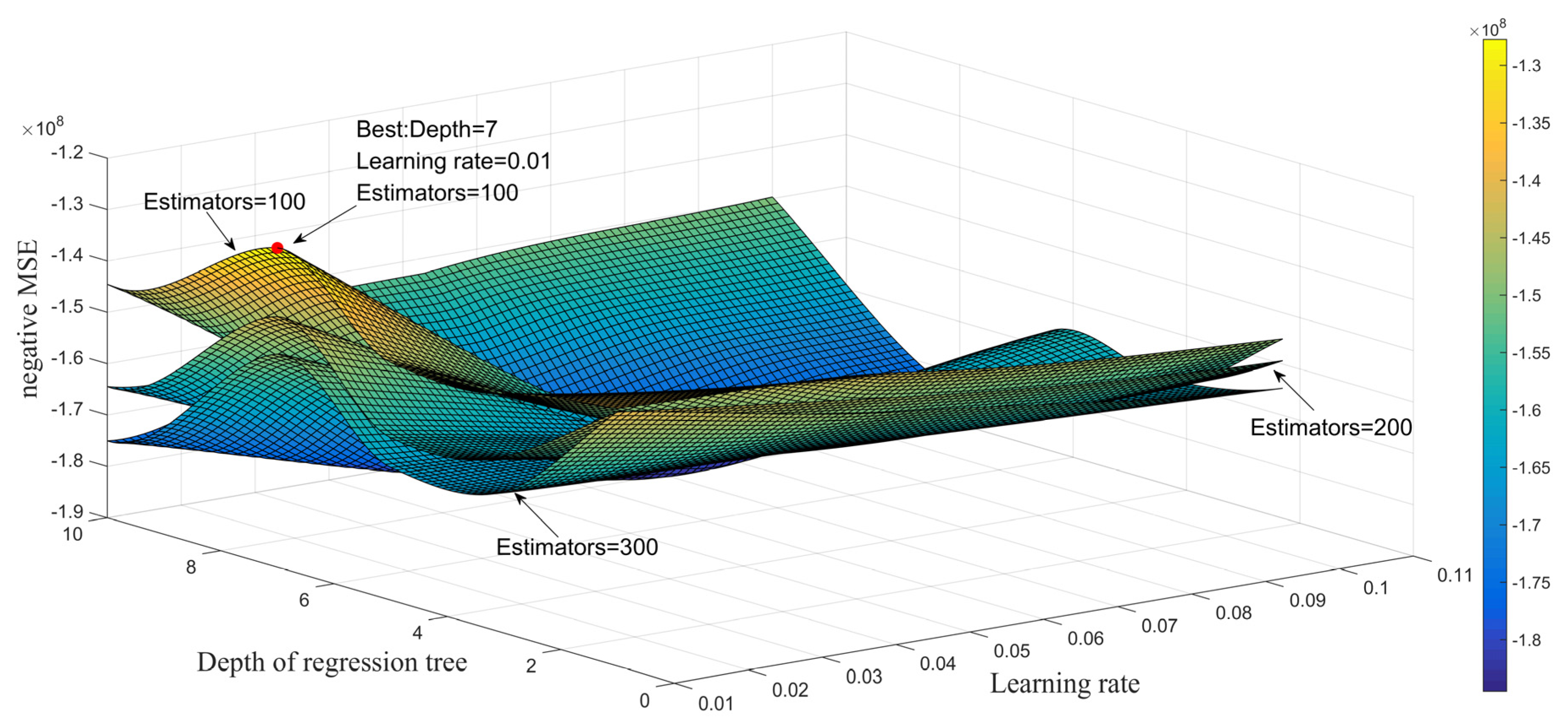
4.1. Determination of Model Hyperparameters

The selection of hyperparameters in the model largely determines the prediction effect. In existing studies, the determination of hyperparameters mainly relies on experience and lacks a practical basis [33], which may lead to a low fit between the model and sample, affecting the overall effect of the model. In this study, the GridSearch method was used to cross-verify and evaluate all combinations of hyperparameters, and the F1 score was used as the distinguishing criterion to optimize the three hyperparameters of the GBDT model: the learning rate, maximum number of decision trees, and tree depth. The parameter-tuning process is illustrated in Figure 2.

The selection of the hyperparameters of the model determines its regression effect to a large extent. The existing hyperparameter determination methods are too subjective, leading to a low degree of fit between the model and the sample, thus affecting the prediction accuracy. In this study, the GridSearch method (GridSearchCV) was used to evaluate all combinations of high parameters through cross-validation, and the mean square error (MSE) was used as the standard to determine the learning rate, maximum number of decision trees, and tree depth of the GBDT model.

The cross-validation function in scikit-learn uses a utility function (bigger is better) rather than a cost function (smaller is better); thus, the model evaluation function is a negative MSE function. All of the combinations of these three groups of hyperparameters are enumerated by the GridSearchCV, generate plenty of GBDT model variants, and calculate their MSE. We visualize this process, and it can be observed that the highest point in Figure 2 (the red dot on the graph) is the model with the smallest MSE; hence, we adopted this model variant as the final model, and the model hyperparameters in this study were as follows: the maximum number of regression trees was 100, the depth of regression trees was 7, and the learning rate was 0.01.

4.2. Overall Effect Analysis and Discussion

This paper discusses the mileage of EVs, a continuous variable, which causes a regression problem. To conduct a comparative analysis, the GBDT model and multiple linear regression models were constructed simultaneously. The two models differ in terms of the solving methods. The GBDT model is solved by the scikit-learn library in Python, whereas ordinary least squares (OLS) is solved using SPSS. The overall results of the model are presented in

Table 3. Overall results of the model.

Variables	GBDT		OLS
	Relative Importance	Cumulative Importance	Estimated Coefficient	Impact
Charging time	18.37%	18.37%	−2.24	−
Charging pile density	15.24%	33.61%	1.84	+
EV preference	11.52%	45.13%	0.98	+
Distance	10.28%	55.41%	0.52	+
Road density	7.61%	63.02%	1.07	+
Public transport service level	7.43%	70.45%	−0.84	−
Annual income	7.27%	77.72%	0.47	+
Land use mix	6.36%	84.08%	−0.36	−
Public transport preference	4.77%	88.85%	−0.13	−
Age	4.41%	93.26%	−0.32	−
Intersection density	3.68%	96.94%	−0.09	−
Population density	3.06%	100.00%	0.04	+
MAPE	9.62%		21.34%

Note: Distance means distance to the nearest business district.

. This table is arranged in descending order of importance of variables, and the errors (MAPE) of the GBDT and OLS models are 9.62% and 21.34%, respectively. It can be seen that the GBDT model is significantly better than the traditional OLS model in terms of the classification effect, indicating that the nonlinear model can better capture the change trend of eVMT.

4.3. Marginal Effect Analysis and Discussion

Based on the PDP method in the GBDT model, the nonlinear relationship between the explanatory variables and EV usage intensity was discussed from the perspective of the built environment and individual travel characteristics. Among them, the built environment variables were summarized according to the 5D concept, and the non-built environment variables were classified by comparison, which were expanded from the charging characteristics of EVs (Figure 3), traffic design (Figure 4), location, population density (Figure 5), public transport service level and diversity (Figure 6), demographic variables (Figure 7), and individual travel characteristics of travel preferences (Figure 8).

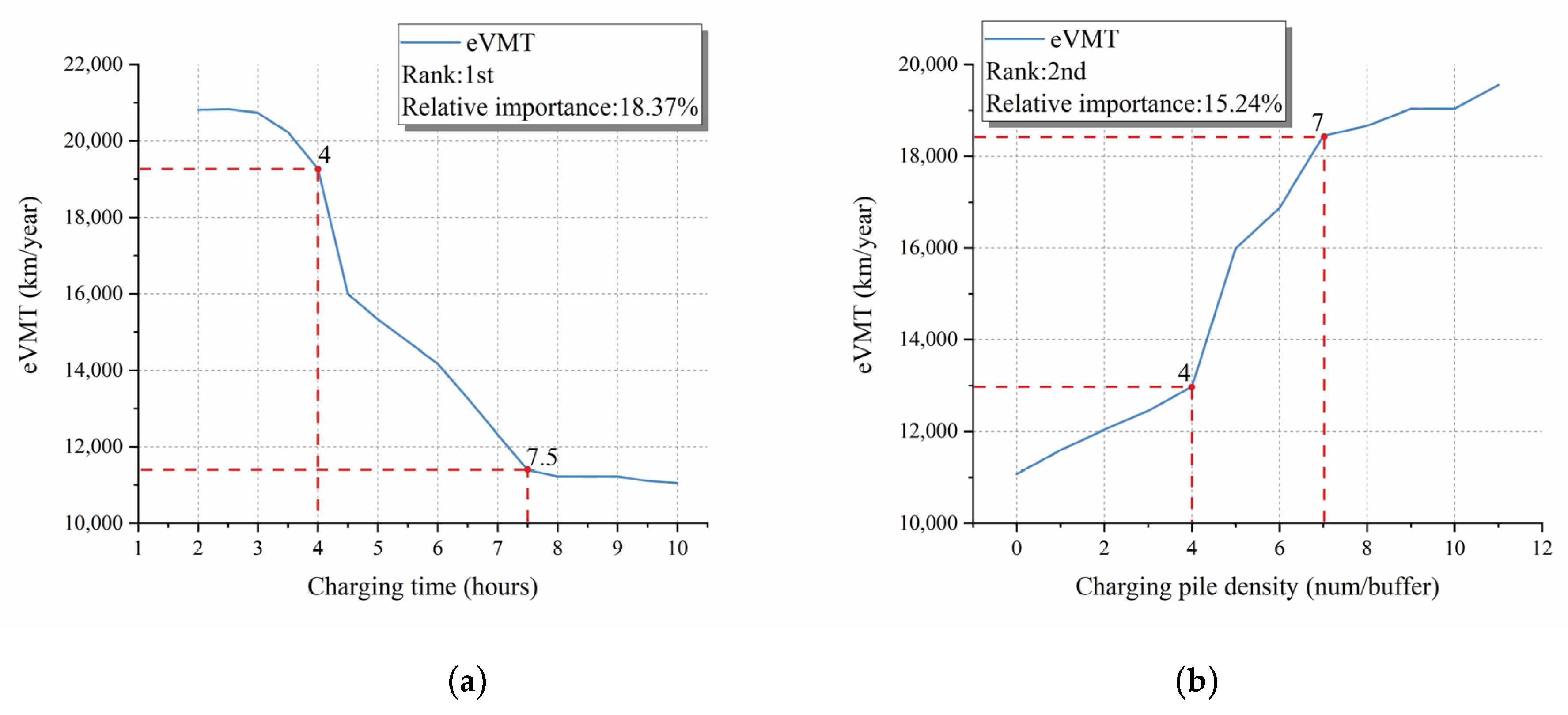
4.3.1. Charging Characteristics of EVs

The relationship between the eVMT and EV charging characteristics is described by the charging duration and the charging pile density. Among the influencing variables of the eVMT, the charging characteristics of the EVs are the most important, with the charging duration having the greatest influence (18.37%) and the charging density having the second greatest influence (15.24%), indicating the cumulative importance of the two indicators reaching 33.61%. As shown in Figure 3a, for EV users, the charging time has a significant negative impact on the driving mileage of EVs. The longer it takes to charge an electric car, the fewer owners will use EVs. Additionally, the influence of the charging duration on the eVMT has a prominent threshold effect. When the charging duration is between 4 h and 7.5 h, the eVMT decreases the most sharply, and the eVMT fluctuation range reaches 8000 km/year, indicating that people are most sensitive to the charging duration during this period. The eVMT showed a slowly decreasing trend from 2 to 4 h and 7.5 h later. This confirms that the slow promotion process of EVs is largely due to the limitation of the current charging time of the EVs, which is consistent with most of the conclusions from the current literature. Figure 3b shows that the charging pile density is positively correlated with the eVMT. Moreover, it can be observed from Figure 3b that, within the range of 4–7 num/buffer, the eVMT changes the fastest, indicating that EV owners are the most sensitive in this range. When the density exceeds 7 num/buffer, eVMT maintains a slow but steady growth, further reflecting the promoting effect of the charging pile density on EV use. Therefore, according to the numerical analysis, it is suggested that the charging pile density is controlled within the range of 7 num/buffer, which is more conducive to the development of EVs.

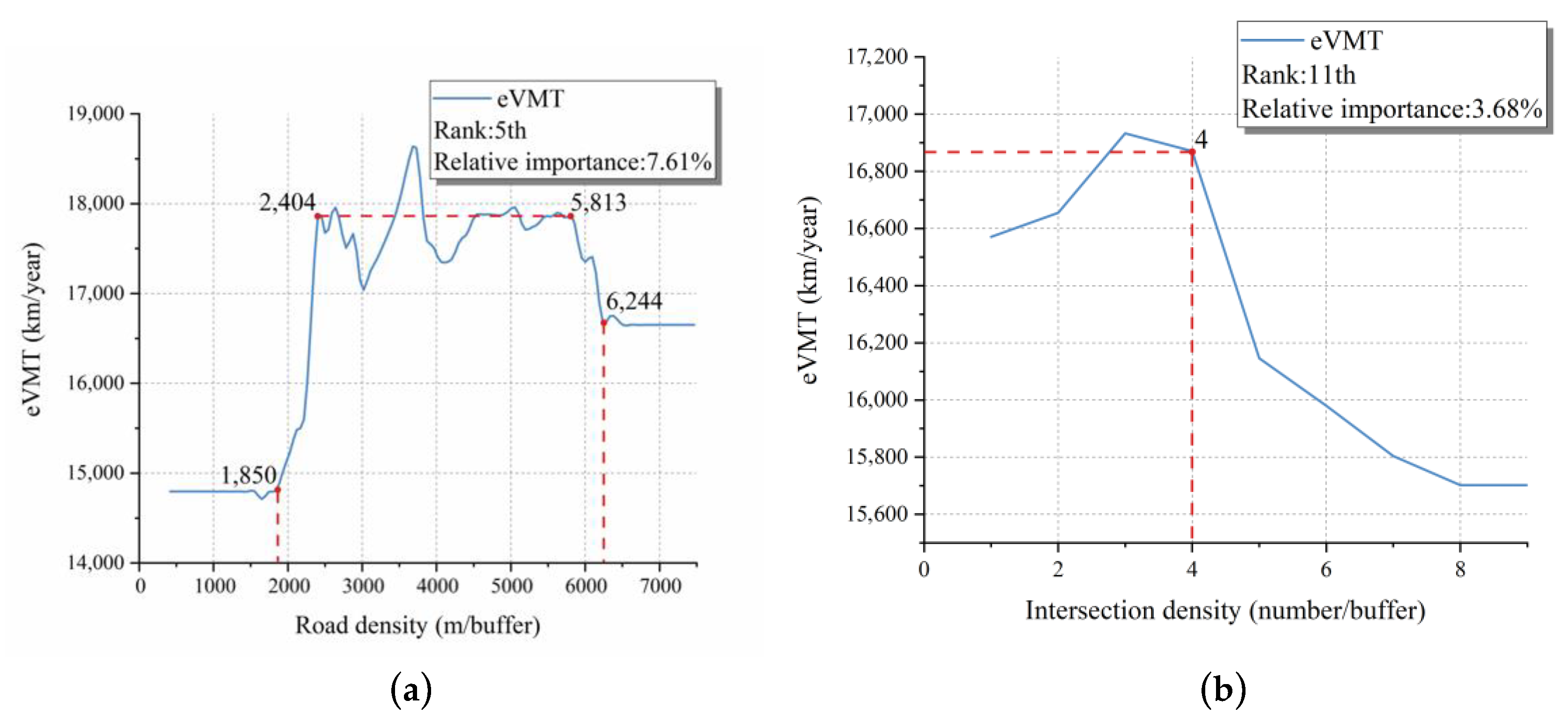
4.3.2. Traffic Design

The intersection and road densities were adopted to measure the traffic design. In the model, these two indicators ranked fifth and eleventh among the twelve influencing variables, respectively, with some differences in importance. First, the road network density represents the ratio of the total road length to the regional area in a certain area centered on residential areas, which is an index reflecting the density of the road network in the area. When describing the influence of the relationship between the road density and eVMT, it can be observed from Figure 4a that the overall image is inverted and U-shaped, that is, a road network density that is too high or too low reduces the use intensity of EVs. A low road network density (road network density less than 1850 km/year) is associated with low destination accessibility, whereas a high road network density (road network density more than 6244 km/year) is associated with an improvement of the bus service level, which induces negative travel effects, such as traffic congestion. However, when the road network density is in the range of 2404–5813 km/year, the annual eVMT fluctuates in the range of 17,000–18,500 km/year. In contrast to the road network density, it can be observed from Figure 4b that the intersection density and eVMT have a positive influence before the buffer reaches the critical value of four intersections and begins to show a significant negative influence once the critical value is exceeded. Within the four intersections, an increase in the number of intersections accompanied by an increase in the road network density improves the destination accessibility index to a certain extent, which is the main reason for the positive impact of intersection density and eVMT. After reaching four intersections, the growth of intersections creates more traffic signal control, which significantly reduces the respondents’ willingness to use EVs. By comparing the slope of change before and after the critical value, it can be deduced that respondents are more sensitive to the inconvenience caused by increasing intersections than to the improvement of destination accessibility, which is similar to the framing effect proposed by Daniel Kahneman [34].

4.3.3. Distance to the Nearest Business District and Population Density

When the eVMT is described by the actual distance between the traveler’s residence and the nearest business district, it can be observed from Figure 5a that the relationship between the distance to the nearest business district and the use intensity of EVs is a zigzag graph and is positively correlated with the overall trend. In terms of importance data, it ranks fourth among the 12 variables, accounting for 10.28%, indicating a relatively high importance. When the distance is within 8 km, there is an obvious threshold effect between the distance (to the nearest business district) and the eVMT, and an overall trend of a positive correlation. Within 8 km, the eVMT reaches small peaks at 1.89 km, 2.97 km, and 5.04 km, respectively. The fluctuation of these three small peaks is mainly related to the bus service level and land use diversity near the residential area, and the existence of such factors leads to an increase in people’s willingness to travel by non-EVs. When reaching 6.7 km, the growth rate of the eVMT slows down, indicating that the travelers’ sensitivity to the business circle distance gradually decreases at this stage. After reaching 8 km, the influence of this indicator on the eVMT gradually disappears, mainly because the increase in the EV travel cost caused by the long-distance business circle exceeds the acceptable range of owners. In terms of population density, it had the lowest importance (3.06%). As shown in Figure 5b, with an increase in population density, the eVMT exhibited a sharp and unstable growth. When the population density reaches 15,000 persons/km², the influence of the eVMT reaches saturation and remains at a stable value of approximately 17,200 km/year, which suggests that the positive impact of the population density on the EV use intensity is within the limit of 15,000 persons/km². This is mainly due to the increase in the public transport load caused by the growth of population density and the increase in people’s preferences for private car travel under the change of demand relationship. Although there are fluctuations, the curve trend is mainly positive, reflecting that an increase in the population density promotes the use intensity of EVs.

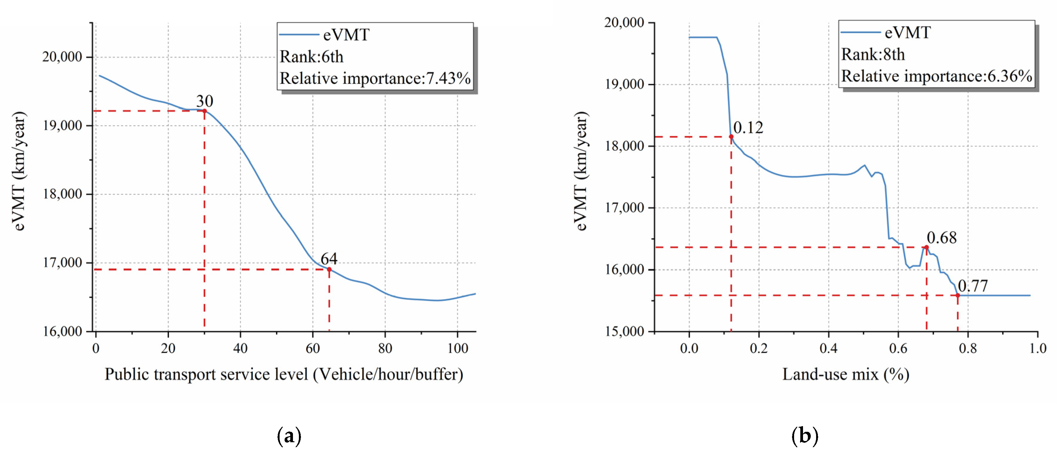
4.3.4. Public Transport Service Level and Diversity

Figure 6a illustrates the nonlinear influence relationship between the public transport service level and eVMT. As described in Figure 6a, the overall influence of the bus service level in the residential buffer zone is clear. When the public transport service level of the buffer is within 30 vehicles/h/buffer, the use intensity of the EV decreases slowly. Once the value is exceeded, the rate of decrease accelerates. When the public transport service level of the buffer is greater than 64 vehicles/h/buffer, its downward trend slows down again and gradually stabilizes. Therefore, this indicates that the sensitive range of respondents using EVs affected by the public transport service level is between 30 and 64 vehicle/hour/buffer. However, the change in the eVMT in the image is in the range of 16,000–20,000 km/year, which is much smaller than that in Figure 6b, indicating that, although the impact of the public transport service level on the eVMT is important, it is very limited. Diversity is measured by the degree of land use mixing, which is relatively low in the model, accounting for 6.36%. From Figure 6b, the image of the land use mix degree and eVMT presented a “ladder shape” with a relatively significant negative impact. The eVMT began to decline significantly at 0.12%, 0.5%, and 0.68% land use mix, respectively. However, in the range of 0.12–0.50%, the change in the land use mix degree did not cause a significant change in the eVMT. Within this range, the eVMT began to decrease slowly and gradually remained stable at approximately 17,500 km/year. This indicates that the impact of the land use mixing degree on the eVMT reaches saturation at the critical value of 0.77%, at which the eVMT is stable at 15,500 km/year.

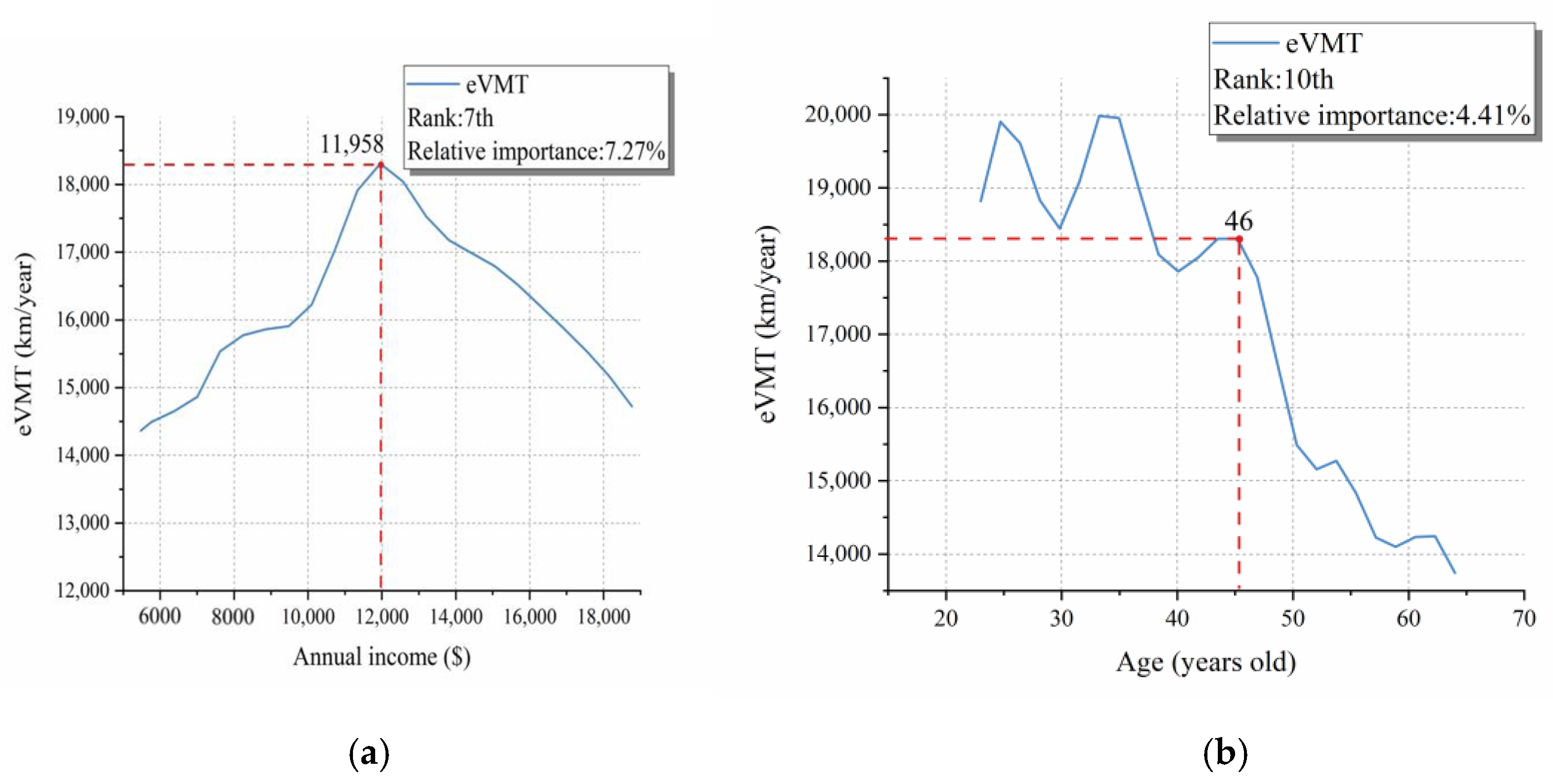
4.3.5. Demographic Variables

Demographic variables were calculated using annual income and age, among which annual income had a medium influence on eVMT, whereas age had a low influence. From Figure 7a, for respondents with an annual income of less than USD 11,958, the higher the annual income, the higher the eVMT, and the growth trend showed a step-growth. For people with an annual income of more than USD 11,958, the higher the annual income, the smaller the eVMT, and the corresponding image slope is relatively stable. There are two main reasons for this difference: people with an annual income of less than USD 8000 have a relatively low income, and the use intensity of EVs is slightly lower than that of people with higher income levels due to the travel cost limitation of EVs. In contrast, people with an annual income above USD 11,958 have more travel vehicle choices than people with an income level below USD 11,958. Therefore, under the condition that people have a higher income, the eVMT of a single EV of a crowd will be lower. From Figure 7b, the use intensity of EVs used by the group younger than 46 years of age is relatively irregular, and the eVMT remains within the range of 18,000–20,000 km/year. However, for the group over 46 years old, the use intensity of EVs decreases significantly, and there is a nonlinear relationship in which the use intensity of EVs decreases with age. The main reason for this is that young people are more receptive to new things and technologies than older people.

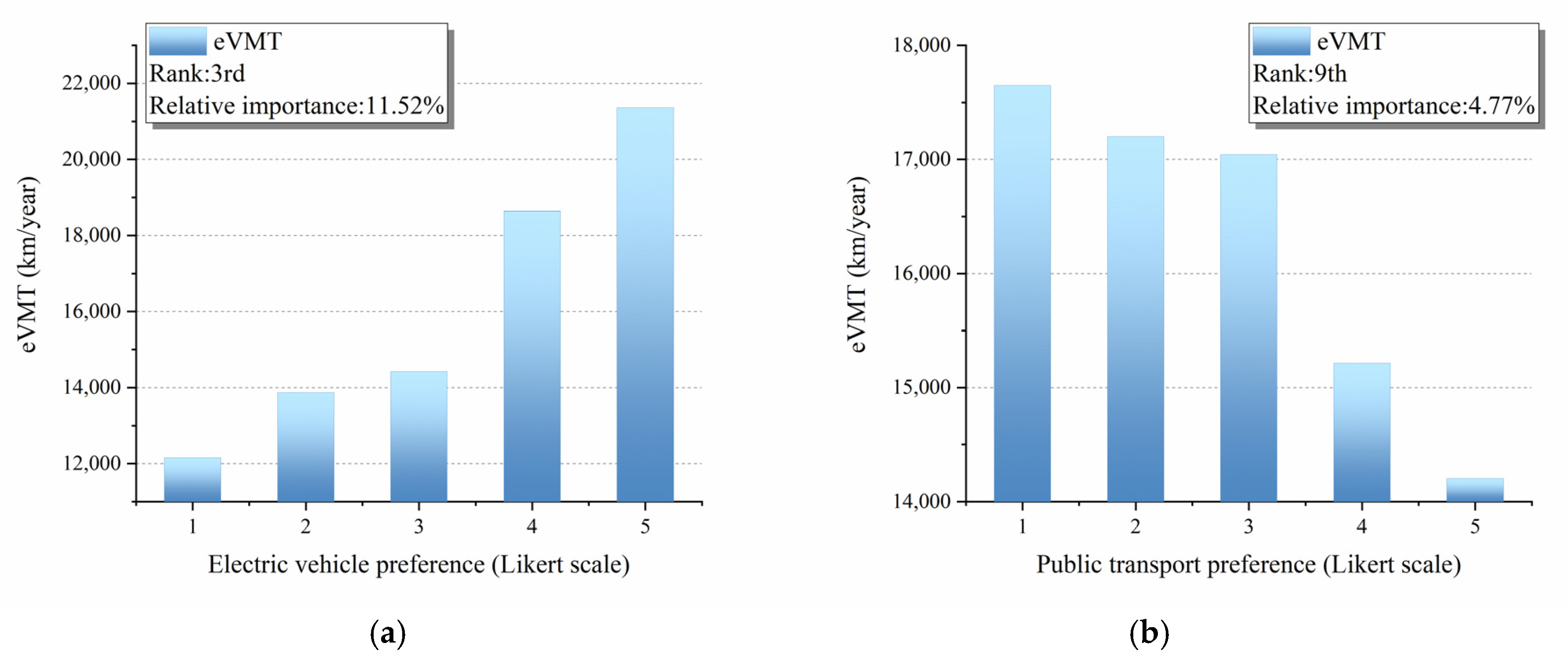
4.3.6. EV Preference and Public Transport Preference

Figure 8 shows the impact of two different travel mode preferences on the eVMT using a five-point Likert scale to measure both variables. Among them, the EV preference has a high degree of influence on the eVMT, accounting for 11.52%, ranking third. In contrast, public transportation preference ranked ninth with a 4.77% importance. The scale from 1 (1 indicates that the individual has no preference for this travel mode at all) to 5 (5 indicates that the individual has a significant preference for this travel mode), indicating an increase in the corresponding preference degree. From Figure 8a, the preference of EVs has a significant promotion effect on the use intensity of EVs, whereas in Figure 8b, the preference for public transportation has a significant hindrance effect on the use intensity of EVs. The similarity between the two images is that the eVMT starts to change significantly at the critical value in Table 3, but the difference lies in the different mapping ranges. The range of preference mapping for EVs is 12,000–22,000 km/year, whereas that of public transportation is 14,000–18,000 km/year. This result further reflects the difference in the importance of the two different preferences when acting on the eVMT.

5. Conclusions

Based on eVMT survey data, this study modeled the use intensity of passenger EVs. The overall results of the model showed that the classification accuracy of the GBDT model was better than that of the traditional OLS model, and the nonlinear model could better capture the variation trend of the individual eVMT. Second, the relative importance indicates that the charging duration (18.37%) and charging pile density (15.24%) are important factors affecting the parking demand of travelers. Similarly, EV preferences (11.52%) and distance to the nearest business district (10.28%) also had a significant influence.

This paper has following originality and merits: First, the relationship between eVMT and built environment is studied, which was not studied previously; second, the GBDT method was applied in the analysis of eVMT influencing factors, and the hyperparameters of the model were optimized, which were not used in this field; third, based on the conventional built environment variables, we added features introduced with EVs charging pile density and the charging time variables, an important contribution of this study. However, it is worth noting that, as a typical modern Chinese city, Chongqing has similar characteristics with the development of China’s urbanization. Therefore, this paper is a positive exploration of the use intensity of EVs, and it is recommended that more studies on eVMT should be conducted in more cities in the future to obtain more general studies.

Finally, based on the research results, from the perspective of promoting EVs, combined with the significant influencing factors of eVMT, we provide the following suggestions:

• Scientifically planning the number of charging piles in a residential area (maintain at least four within 500 m of the residential area charging piles).
• Accelerating the research and development of fast-charging EVs (ensure that the average charging time of EVs is within 7.5 h; within 4 h is the best).
• Areas with a high road density (over 2404 m/buffer), high intersection density (over 4 num/buffer), and residential areas far away from business districts or areas with a population density of approximately 15,000 person/km² should invest more EVs promotion costs.
• Carry out more sales promotion for those with an annual income of about USD 11,958 and the young and middle-aged population.

References

1. Acciaro, M.; Ghiara, H.; Cusano, M.I. Energy management in seaports: A new role for port authorities. Energy Policy 2014, 71, 4–12. [Google Scholar] [CrossRef]
2. Jacobson, M.Z. Review of solutions to global warming, air pollution, and energy security. Energy Environ. Sci. 2009, 2, 148–173. [Google Scholar] [CrossRef]
3. Amelung, D.; Helen, F.; Alina, H.; Carlo, A.; Louis, V.R.; Heiko, B.; Wilkinson, P.; Sauerborn, R. Human health as a motivator for climate change mitigation: Results from four European high-income countries. Glob. Environ. Chang. 2019, 57, 101918. [Google Scholar] [CrossRef]
4. Darabi, Z.; Ferdowsi, M. Impact of plug-in hybrid electric vehicles on electricity demand profile. IEEE Trans. Sustain. Energy 2011, 2, 501–508. [Google Scholar] [CrossRef]
5. Nian, V.; Hari, M.P.; Yuan, J. A new business model for encouraging the adoption of electric vehicles in the absence of policy support. Appl. Energy 2019, 235, 1106–1117. [Google Scholar] [CrossRef]
6. Ewing, R.; Cervero, R. Travel and the built environment. J. Am. Plan. Assoc. 2010, 76, 265–294. [Google Scholar] [CrossRef]
7. Cervero, R.; Kara, K. Travel demand and the 3ds: Density, diversity, and design. Transp. Res. D 1997, 2, 199–219. [Google Scholar] [CrossRef]
8. Ewing, R.; Cervero, R. Travel and the built environment: A synthesis. Transp. Res. Rec. 2001, 1780, 87–114. [Google Scholar] [CrossRef] [Green Version]
9. Ewing, R.; Greenwald, M.J.; Zhang, M.; Walters, J.; Feldman, M.; Cervero, R.; Thomas, J. Measuring the Impact of Urban Form and Transit Access on Mixed Use Site Trip Generation Rates—Portland Pilot Study; US Environmental Protection Agency: Washington, DC, USA, 2009.
10. Singh, A.C.; Astroza, S.; Garikapati, V.M.; Pendyala, R.M.; Bhat, C.R.; Mokhtarian, P.L. Quantifying the relative contribution of factors to household vehicle miles of travel. Transp. Res. D 2018, 63, 23–36. [Google Scholar] [CrossRef]
11. Sardari, R.; Shima, H.; Raha, P. Effects of traffic congestion on vehicle miles traveled. Transp. Res. Rec. 2018, 2672, 92–102. [Google Scholar] [CrossRef]
12. Macioszek, E. Electric Vehicles—Problems and Issues. Smart and Green Solutions for Transport Systems, Transport Systems. Theory and Practice 2019; Springer: Katowice, Poland, 2020. [Google Scholar]
13. Macioszek, E. E-mobility Infrastructure in the Górnolsko—Zagbiowska Metropolis, Poland, and Potential for Development. In Proceedings of the 5th World Congress on New Technologies, Lisbon, Portugal, 18–20 August 2019. [Google Scholar]
14. Gandoman, F.H.; Ahmed, E.M.; Ali, Z.M.; Berecibar, M.; Zobaa, A.F.; Shady, H.E.A.A. Reliability Evaluation of Lithium-Ion Batteries for E-Mobility Applications from Practical and Technical Perspectives: A Case Study. Sustainability 2021, 13, 11688. [Google Scholar] [CrossRef]
15. Weiller, C. Plug-in hybrid electric vehicle impacts on hourly electricity demand in the United States. Energy Policy 2011, 39, 3766–3778. [Google Scholar] [CrossRef]
16. Ling, Z.W.; Cherry, C.R.; Wen, Y. Determining the Factors That Influence Electric Vehicle Adoption: A Stated Preference Survey Study in Beijing, China. Sustainability 2021, 13, 11719. [Google Scholar] [CrossRef]
17. Gardner, B.; Abraham, C. What drives car use? a grounded theory analysis of commuters’ reasons for driving. Transp. Res. F 2007, 10, 187–200. [Google Scholar] [CrossRef]
18. Gardner, B.; Abraham, C. Psychological correlates of car use: A meta-analysis. Transp. Res. F 2008, 11, 300–311. [Google Scholar] [CrossRef]
19. Jiang, Q.; Wei, W.; Xin, G.; Dexin, Y. What increases consumers’ purchase intention of battery electric vehicles from Chinese electric vehicle start-ups? taking Nio as an example. World Electr. Veh. J. 2021, 12, 71. [Google Scholar] [CrossRef]
20. Ewing, G.O.; Emine, S. Car fuel-type choice under travel demand management and economic incentives. Transp. Res. D 1998, 3, 429–444. [Google Scholar] [CrossRef]
21. Krishnan, V.V.; Koshy, B.I. Evaluating the factors influencing purchase intention of electric vehicles in households owning conventional vehicles. Case Stud. Transp. Policy 2021, 9, 1122–1129. [Google Scholar] [CrossRef]
22. Mohamed, N.; Aymen, F.; Ali, Z.M.; Zobaa, A.F.; Shady, H.E.A.A. Efficient Power Management Strategy of Electric Vehicles Based Hybrid Renewable Energy. Sustainability 2021, 13, 7351. [Google Scholar] [CrossRef]
23. Guan, H.Z.; Liu, R.Y.; Zeng, M.Y. Park-and-ride transfer behaviors under the circumstances of insufficient park-and-ride parking space. J. Beijing Univ. Technol. 2019, 45, 593–600. [Google Scholar]
24. Meng, F.; Yuchuan, D.; Yuen, C.L.; Wong, S.C. Modeling heterogeneous parking choice behavior on university campuses. Transp. Plan. Technol. 2018, 41, 154–169. [Google Scholar] [CrossRef]
25. Yiming, X.; Yan, X.; Liu, X.; Zhao, X. Identifying key factors associated with ride splitting adoption rate and modeling their nonlinear relationships. Transp. Res. A 2021, 144, 170–188. [Google Scholar]
26. Cervero, R. Built environments and mode choice: Toward a normative framework. Transp. Res. D 2002, 7, 265–284. [Google Scholar] [CrossRef]
27. Zhong, H.M.; Zhang, W.L.; Li, Y.R.; Zhu, Z.F.; Zhao, Y. GBDT based railway accident type prediction and cause analysis. Acta Autom. Sin. 2021, 47, 1–9. [Google Scholar]
28. Li, W.Z.; Yang, L.L.; Wen, Z.; Chen, J.L.; Wu, X. On the optimization strategy of EV charging station localization and charging piles density. Wirel. Commun. Mob. Comput. 2021, 99, 6675841. [Google Scholar] [CrossRef]
29. Ding, C.; Cao, X.Y.; Naess, P. Applying Gradient Boosting Decision Trees to Examine Non-Linear Effects of the Built Environment on Driving Distance in Oslo. Transp. Res. A 2018, 110, 107–117. [Google Scholar] [CrossRef]
30. Zhang, W.J.; Zhao, Y.J.; Cao, X.Y.; Lu, D.M.; Chai, Y.W. Nonlinear Effect of Accessibility on Car Ownership in Beijing: Pedestrian-Scale Neighborhood Planning. Transp. Res. D 2020, 86, 102445. [Google Scholar] [CrossRef]
31. Ding, C.; Cao, X.Y.; Liu, C. How Does the Station-Area Built Environment Influence Metrorail Ridership? Using Gradient Boosting Decision Trees to Identify Non-Linear Thresholds. J. Transp. Geogr. 2019, 77, 70–78. [Google Scholar] [CrossRef]
32. Chen, E.; Ye, Z.; Wu, H. Nonlinear effects of built environment on intermodal transit trips considering spatial heterogeneity. Transp. Res. D 2021, 90, 102677. [Google Scholar] [CrossRef]
33. Christiansen, P.; Øystein, E.; Nils, F.; Jan, U.H. Parking facilities and the built environment: Impacts on travel behaviour. Transp. Res. A 2017, 95, 198–206. [Google Scholar] [CrossRef]
34. Peng, J.X.; Jiang, Y.; Miao, D.M.; Li, R.; Xiao, W. Framing effects in medical situations: Distinctions of attribute, goal and risky choice frames. J. Int. Med. Res. 2013, 41, 771–776. [Google Scholar] [CrossRef] [PubMed]
Figure 1. Distribution map of residential spots of survey sample.
Wevj 12 00247 g001
Figure 2. Hyperparameters adjustment process.
Wevj 12 00247 g002
Figure 3. Relationship between EV charging characteristics and eVMT: (a) Charging time with eVMT; (b) Charging pile density with eVMT.
Wevj 12 00247 g003
Figure 4. Relationship between traffic design and eVMT: (a) Road density with eVMT; (b) Intersection density with eVMT.
Wevj 12 00247 g004
Figure 5. Influence of distance to the nearest business district and population density on eVMT: (a) Distance to nearest bussiness district with eVMT; (b) Population density with eVMT.
Wevj 12 00247 g005
Figure 6. Influence of public transport service level and land use mix on eVMT: (a) Public transport service level with eVMT; (b) Land-use mix with eVMT.
Wevj 12 00247 g006
Figure 7. Influence of demographic variables on eVMT: (a) Annual income with eVMT; (b) Age with eVMT.
Wevj 12 00247 g007
Figure 8. Influence of public transport service level and land use mix on eVMT: (a) Electric vehicle preference with eVMT; (b) Public transport preference with eVMT.
Wevj 12 00247 g008