Real Driving Range in Electric Vehicles: Influence on Fuel Consumption and Carbon Emissions

Abstract

This paper is focused on the determination of real driving ranges for electric vehicles (EV’s) and how it influences fuel consumption and carbon emissions. A precise method to evaluate the driving range of an EV can establish the correct reduction in GEI amount, mainly CO and CO₂, ejected to the environment. The comparison of the daily driving range between an internal combustion engine (ICE) vehicle and an EV provides a useful tool for determining actual fuel saved during a daily trip and a method to compute carbon emissions saved depending on the type of ICE vehicle. Real driving range has been estimated on the basis of a daily trip consisting of five different segments, acceleration, deceleration, constant speed, ascent and descent, which reproduce the different types of driving. The modelling has been developed for urban routes since they are the most common and the most polluted environment where the use of electric vehicles is applied. The effects of types of driving have been taken into account for the calculation of the driving range by considering three main types of driving: aggressive, normal and moderate. The types of vehicle in terms of shape and size as well as dynamic conditions and the types of roads have also been considered for the determination of the driving range. Specific software has been developed to predict electric vehicle range under real driving conditions as a function of the characteristic parameters of a daily trip.

1. Introduction

Electric vehicles are today’s main alternative to internal combustion engine (ICE) vehicles. The transition from ICE to EV involves studying the retrofit method to improve the transition from ICE to EV [1] and analyzing different factors such as life cycle assessment (eLCA) [2] or life cycle costing (LCC) to decide whether or not the transition from ICE to EV is suitable [3]. The comparison of the influence of the different types of car powered (EV, H₂ or ICE) from decarbonized fuels is also under consideration in terms of adopting a future model of road transportation [4]. This transition is especially interesting in urban routes, since they do not produce carbon emissions, thus reducing pollution level and helping to tackle climatic change [5,6]. The progressive replacement of ICE vehicles by hybrid electric vehicles (HEV), plug-in electric vehicles (PHEV) and full electric vehicles (EV) has contributed to reducing urban carbon emissions. Some studies have been devoted to the analysis of the reduction in greenhouse gas emissions by using modelling processes where ICE vehicles have been replaced by EV, HEV or FC vehicles in urban environments [7]; others use artificial intelligence (AI) applied to plug-in electric vehicles (PHEV) in order to optimize vehicle configuration and its influence on the air pollution [8]. The benefits of a transition to vehicle electrification onto the citizens’ health is another point of interest to consider in a decision on the change of transport model in urban areas [9]. Furthermore, the use of EV may influence the population distribution as well as the use of the land through changes in transport demand, type of energy use and emission profiles, which affects the concentration of pollutant gasses and, thus, human welfare [10]. Simulation studies have been conducted to estimate the reduction in gas emissions in highly concentrated urban areas [11]. The influence of driving regulations onto some of the aforementioned issues has also been studied [12]. Additional benefits derived from the use of EV, such as a lower local environmental temperature, reduced AC energy requirements [13]. Finally, some investigations have been focused on the minimization of global and local environmental impact due to the use of EV, among other factors [14].

Currently, one of the main worries of electric vehicle manufacturers is the range of autonomy, either for full electric vehicles, plug-in electric vehicles or hybrid electric vehicles. Many studies have been devoted to this problem and are supported by public and private research institutions, providing a database that is used by car manufacturers [15,16,17]. Private companies develop their own tests to determine the driving range of an electric vehicle with the subsequent different results; tests, however, have been normalized according to specific protocols such as NEDC, WLTP, FTP-75 and JP-08 (see Section 3), although some studies have developed a simulation process to take into account the different factors affecting the electric vehicle range [18]. The driving range of an electric vehicle, however, is not a constant value, as it depends on many factors such as driving mode [19,20], road type [21], traffic environment [22], battery aging [23,24], etc.; therefore, the real value currently differs from car manufacturer data.

Driving range depends on battery capacity provided that the aforementioned factors remain unchanged, thus the higher capacity results in longer range. Nevertheless, battery capacity is not constant since it evolves with discharge rate and power demand, resulting in variable autonomy and driving range. The effects of the discharge rate have been widely studied by many authors analyzing the different factors that modify battery capacity due to operating conditions [25,26,27,28,29].

Although driving range has been improved in the last years, it continues to be the most important challenge that researchers and the industry have to confront in order to make electric vehicles competitive. By comparing driving ranges with internal combustion engine vehicles, it is observed that the ones for EV are still low, especially in interurban routes. Despite the fact that urban routes are relatively well covered by today’s EV autonomy, a more adaptive performance of EV car batteries relative to real conditions can enlarge the driving range, thus improving the time of single use.

Driving range is essential for computing carbon emission reduction in urban areas since the evaluation of the emitting gases of greenhouse effects (GEI) such as CO and CO₂ coming out from the exhaust pipes of ICE vehicles is directly related to the driving distance; therefore, the precise knowledge of the driving range of an electric vehicle results in the accurate determination of carbon emissions reduction.

The reduction in carbon emissions depends on the type of ICE vehicle [30,31]; however, based on statistical data, an estimation of the average emissions by ICE cars in urban areas may be useful for calculations [32,33,34,35,36,37]. Moreover, the use of electric vehicles also contributes in reducing fuel consumption [38,39,40], which generates a preservation of the environment since the production of fuel for urban traffic also provokes carbon emissions.

The use of full electric vehicles avoids carbon emissions as far as driving the vehicle is concerned, although the electricity required to recharge the batteries produces carbon emissions unless it is generated by renewable energy sources. Nevertheless, other electric vehicles such as hybrid and plug-in vehicles cannot be considered emissions free since they combine an electric engine and an ICE one [41,42].

On the other hand, electric vehicle engines last longer than ICE ones, which represents a global lower emissions rate despite the electricity used for recharging batteries comes from conventional polluting power plants [43].

The method of driving is another point that should be considered in the calculation of the carbon emissions and fuel consumption, since an aggressive mode results in higher fuel consumption and carbon emissions [44,45]. Therefore, fuel consumption saving can be determined from the driving mode and driving dynamic conditions, assuming that both ICE and EV vehicles operate at equal conditions.

2. Fuel Consumption

Fuel consumption is a reference parameter that car manufacturers provide to estimate the driving range of a vehicle. This parameter is given in different units depending on the world zone; in many countries, it is expressed in liters of fuel per 100 km of driving trip (l/100 km); however, the American market uses mileage (mpg) as the unit to express fuel consumption, which indicates how many miles can be driven per gallon of consumed fuel.

The estimated driving range is calculated on the basis of the average fuel consumption, which never occurs since the driving conditions vary along the driving trip; this situation only results in an approximate driving range for any vehicle and a real range is never known. In fact, the driving range is always lower than estimated from standard fuel consumption, which is a very common complaint among the drivers; therefore, in order calculate fuel consumption within high accuracy, it is necessary to apply real driving conditions to the calculation.

The standard method for the estimation of the driving range in an ICE vehicle uses the following expression.

$$DR=TV/FC$$

(1)

DR, TV and FC represent driving range, fuel tank capacity and standard fuel consumption.

In Equation (1), driving range can be expressed in kilometers or miles, depending on the world zone. Fuel tank capacity is indicated in liters or gallons, and fuel consumption should be given in liters per kilometer or gallons per mile. In this latter case, it is necessary to use the inverse of the mileage value, which is the current method for expressing fuel consumption in the English system (miles per gallon (mpg)).

If we take into consideration that the vehicle does not run at constant driving conditions, we should divide the daily trip into segments, each one having specific conditions; therefore, the above expression should be reformulated as follows:

$$DR=TV{\displaystyle \sum _{i=1}^n\frac{{\left(f_V\right)}_i}{{\left(FC\right)}_i}}$$

(2)

$$DR=TV{\displaystyle \sum _{i=1}^n{\left(f_V\right)}_i{\left(FC\right)}_i}$$

(3)

where f_V represents the volume fraction of the fuel tank that has been used for the specific segment i, and n is the number of segments that the daily trip has been divided in.

Coefficient f_V is not easy to measure within high precision, but accuracy can be improved significantly if the appropriate sensor is used. Fuel consumption at every segment, (FC)_i, cannot be considered constant any longer, since driving conditions such as acceleration, deceleration, constant speed, ascent or descent segment results in a variable fuel consumption rate.

Fuel consumption at every segment can be determined using the following equation:

$${\left(FC\right)}_i=\frac{{\xi }_i}{CH}=\frac{P_i{t}_i}{{\eta }_{th}CH}$$

(4)

where ξ_i is the energy consumed in the segment i, P_i the required power, t_i the driving time and CH represents fuel combustion heat in J/kg or BTU/pound. η_th represents the efficiency of the ICE.

It should be noted that the fuel consumption is given in kilograms or pounds. In the case where fuel consumption should be expressed in liters or gallons, Equation (3) is transformed into the following:

$${\left(FC\right)}_i=\frac{P_i{t}_i}{\rho {\eta }_{th}CH}$$

(5)

where ρ represents fuel density in kg/L or pounds/gallon.

Fuel combustion heat depends on the type of fuel, gasoline or diesel and on fuel composition; however, there is not much difference between the different fuels used for ICE vehicles. Provided that the ICE efficiency and fuel combustion heat are known, the fuel consumption only depends on the required power at every daily trip segment. Power is determined from driving dynamic conditions, which can be established as a function of the vehicle speed, tilt of the road, rolling factor between road and tires, shape and size of the vehicle and acceleration rate. In the Theoretical Background Section, the dynamic conditions for a vehicle are analyzed.

3. Driving Cycle Protocol

Among the many driving tests for EV, four are the most relevant: NEDC, WLTP, FTP-75 and JC08. The first two have been developed for the European market while FTP-75 and JC08 are for the American and Japanese markets. Some differences arise when comparing one to another: NEDC (New European Driving Cycle) is mainly devoted for urban routes, although it includes an extra urban driving cycle (EUDC); however, the protocol does not match the real driving conditions in current days, as it is considered too conservative [46]. FTP-75 is also a driving cycle protocol that was developed firstly for urban routes but updated for highway driving (HWFET), aggressive driving (SFTP US06) and optional air conditioning tests (SFTP SC03) [47]. This test is more realistic than NEDC as it includes some of the today’s driving modes in modern cities and developed countries.

The FTP-75 test, however, is developed for the American standard driving conditions, for which its speed limits in many states are a little bit more conservative than European ones [48]. The Japanese JC08 cycle [49] is even more conservative than FTP-75 as far as speed limit is concerned; furthermore, the cycle duration is too short for current modern driving times; therefore, it does not represent a real picture of a single mode of EV driving for today’s drivers. Finally, WLTP (World Harmonized Light-Duty Vehicle Test Procedure) shows up as a solution to fulfil the real requirements of power demand for an EV in modern society, especially for interurban routes: although it is more realistic than the NEDC, the WLTP protocol slightly differs from real driving conditions since the driving conditions under which the protocol run on are based on average driving conditions, which are not completely precise [50,51].

Advanced studies have developed a more accurate model to determine the fuel consumption of electric vehicles under real driving conditions (RDC) [52,53], which improves the accuracy of the determination but does not use online instant values; thus, it does not reflect the specific driving mode associated with any driver. Other models use collected data from real driving conditions [54]. The method provides real data from electric vehicles under various driving conditions, including kinematics aspects and segmentation of the driving trip, in a very similar way than proposed in the present paper, with the difference that the proposed method includes online values of the critical magnitudes.

In summary, due to the specific driving mode that people adopt, a unique driving protocol that could match the driving conditions does not exist; therefore, it is wise to develop an adaptive model that can be applied to changes in driving mode as vehicles and road conditions evolve. This can also be applied to urban routes where traffic regulations may affect the speed limits or time interval of driving before stopping.

4. Modeling

The development of the new driving cycle modeling is based on the consideration that the daily cycle is made up of a group of five steps: normal running at constant speed, acceleration, deceleration, ascending and descending road. These five steps are complemented with the corresponding stops, when necessary, and the regenerative breaking process during descent, if any.

The daily cycle, then, must be divided into these five steps, plus the corresponding stops, in order to match the global time dedicated to the daily urban route. It is assumed that the daily cycle is repeated day after day with no exception. Based on statistical data and the current method of driving in a big city, for which the model has been developed, a specific time has been assigned to every step no matter when the step has occurred during the day. By conducting this, we have grouped all times as a step is produced into a single event, thus simplifying the model development.

At every step, the car has driven a certain distance given by the dynamic conditions of driving; the sum of all distance should provide the global distance of a daily route. In the case where a specific cycle is reproduced, this global distance should match the standard distance of the tested cycle.

5. Methodology

The project should develop a software that allows the user to know the remaining driving distance by setting up the driving conditions from a menu on the control panel. This menu should include the different options that correspond to the driving mode and type of journey. Every option will correspond to the related algorithms that control the driving process and how they influence the performance of the battery; thus, the amount of extracted charge and energy and, consequently, the driving range can be known.

6. Theoretical Background

The autonomy of an electric vehicle depends on the energy consumption rate and on the battery capacity that supplies energy for propelling the vehicle. The energy of the battery is directly related to its operational voltage, while electric vehicle energy consumption can be obtained from the demanded power and time of operation.

Since an electric vehicle does not maintain constant speed at all times, the average value should be obtained using the following equation.

$$<v>=\frac{1}{t_2-t_1}{\displaystyle \underset{t_1}{\overset{t_2}{\int }}v(t)dt}$$

(6)

The speed distribution is not often known as it depends on driving conditions and driving mode, which can be considered randomly variable.

Global force can be expressed as the following:

$$F=ma+k{v}^2+\mu mg+mg\sin \beta$$

(7)

where m is the mass of the vehicle, a the acceleration, k the effective drag coefficient, v the vehicle speed, μ the rolling factor with the road and β the slope of the road.

The first term of the right hand of Equation (7) corresponds to the inertial effects; the second is the drag force due to the wind; the third term refers to the rolling effect between the vehicle tires and the road; and the last term accounts for the force at the tilted sections of the road.

If we consider a daily trip, we should divide the entire route into segments since the driving conditions, speed, acceleration and tilt are not constant at all times. In such a case, the global force must be expressed as the following.

$$F={\displaystyle \sum _{i=1}^n{F}_i}={\displaystyle \sum _{i=1}^n\left(m{a}_i+k_i{v}_i^2+{\mu }_{i}mg+mg\sin {\beta }_i\right)}$$

(8)

In order to simplify the analysis, a constant rolling factor can be considered, assuming the type of road is the same for the entire trip. The effective drag coefficient depends on type of flow and, thus, on Reynolds’ number, given by the following equation.

$$\mathrm{Re}=\left(v{L}_{eq}/\nu \right)$$

(9)

The parameter L_eq represents the equivalent length of the cross section of the vehicle, which is directly dependent on its shape and size, and ν is the kinetic viscosity of air.

If we assume that there is no significant change in vehicle speed along the route, the Reynolds’ number can be considered constant since the air’s viscosity is also constant provided that there are no sudden changes in the air’s temperature, and L_eq can be considered constant because shape and size of the vehicle are not modified. In the case where temperature effects are considered, air viscosity should be modified according to the following expression.

$$\nu =\left[8x{10}^{-5}{\left(t_C\right)}^2+0.0909t_c+13.21\right]\left(x{10}^{-6}{m}^2/s\right)$$

(10)

The Reynolds’ number in Equation (9) should be modified accordingly.

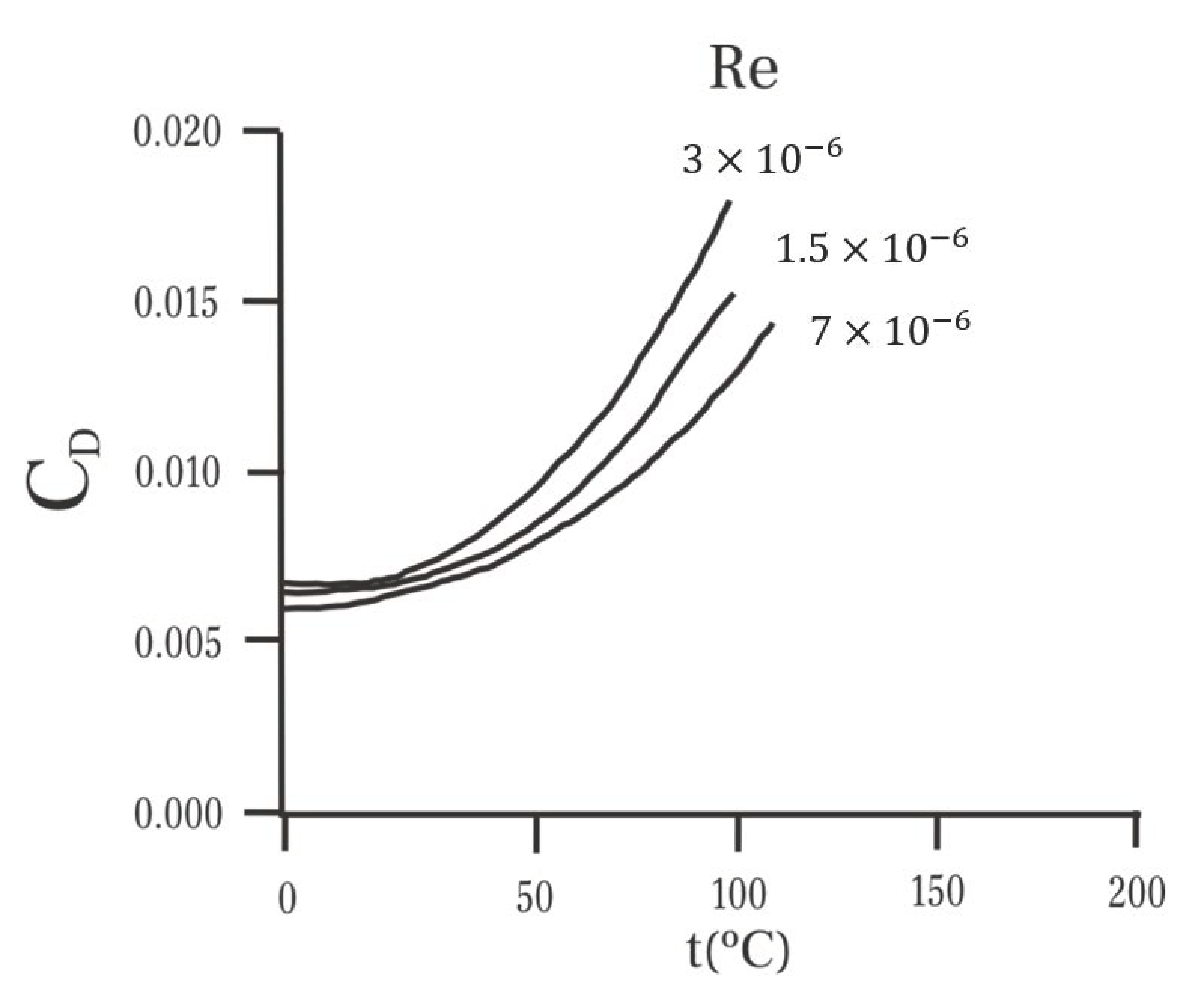
The drag force can be expressed as follows:

$$F_D=k{v}^2=\frac{\rho C_{D}A}{2}{v}^2$$

(11)

where the coefficient, C_D, is dependent on Reynolds number, and the air density is dependent on the temperature, as is described in the following.

$$\rho =\left[-3x{10}^{-8}{\left(t_C\right)}^3+2x{10}^{-5}{\left(t_C\right)}^2-0.0056t_c+1.3\right]\left(kg/m^3\right)$$

(12)

The C_D coefficient barely changes with the Reynolds number for low range of temperature, as it can be observed in Figure 1; in fact, for a temperature change of 50 °C, the C_D coefficient adopts a maximum variation of 3%.

Therefore, if the drag coefficient is considered constant for a relatively wide range of temperature, 0 °C to 40 °C, it is only dependent on air density; thus, the global force expression adopts the following form.

$$F={\displaystyle \sum _{i=1}^n\left(m{a}_i+\rho \frac{C_{D}A}{2}{v}_i^2+\mu mg+mg\sin {\beta }_i\right)}$$

(13)

Power and energy demand to propel the vehicle are supplied by the battery; thus, ξ_EV = ξ_bat. Converting mechanical power into energy is performed by using the following:

$$CV=F<v>\Delta t$$

(14)

from which we obtain the following:

$$CV={\displaystyle \sum _{i=1}^n\left[\left(m{a}_i+k{v}_i^2+\mu mg+mg\sin {\beta }_i\right)<v_i>{\left(\Delta t\right)}_i\right]}$$

(15)

where the time interval, Δt_i, is the duration of every segment of the trip

Battery voltage decays as charge is extracted; thus, the voltage cannot be taken as a constant in Equation (15). To determine the battery voltage at every time, we should know the evolution with respect to time; for lithium batteries, which are the most widely used in electric vehicles, the voltage decay follows a linear pattern that can be expressed as follows:

$$V_i=V_o-s{(DOD)}_i$$

(16)

where V_o is the initial voltage at a fully charged state, s is the slope of the voltage decay line and DOD is the depth of discharge.

The parameter V_o depends on the type and structure of the battery, and it is currently provided by the manufacturer; the slope is obtained from the technical data sheet of the battery, which is also provided by the manufacturer, or experimentally determined. Although the slope of the voltage decay line for any kind of batteries depends on the discharge rate, in the case of lithium batteries, there is only a slight influence; thus, the parameter s can be considered constant between certain limits.

By applying the aforementioned condition, we deduce the following:

$$s=\frac{V_o-V_{off}}{100}$$

(17)

where V_off represents the cut-off voltage of the battery

The depth of discharge is defined as the fraction of charge extracted from the battery related to its global capacity. Global capacity, also called nominal capacity, is the charge a battery can deliver from a fully charged state until completely discharged for a reference time, which is a value that is usually provided by the manufacturer (20 h most of the times).

Since the battery voltage decays for a time interval corresponding to a segment of the trip, Equation (12) must be expressed in the following form.

$$C\left(V_o-V_{off}\right)={\displaystyle \sum _{i=1}^n\left[\left(m{a}_i+k{v}_i^2+\mu mg+mg\sin {\beta }_i\right)<v_i>{\left(\Delta t\right)}_i\right]}$$

(18)

The energy from the battery is transmitted to the electric engine throughout a powertrain that operates at a specific efficiency level depending on the power train configuration. A previous study on this subject [55] shows the efficiency of different powertrain systems operating at different efficiency values depending on the type of protocol, NEDC or HWFET. Since NEDC is very conservative and it is no longer accepted as a reference, the HWFET cycle is used. According to results from the study, the efficiency of the different powertrain configurations is rather constant once the powertrain configuration is set up (see Figure 2).

By using a single motor configuration (SM), we can observe that there is not much difference between the SM1ST or SM2ST configuration, with an average value of 85% for the entire interval. Therefore, we can use this value as a reference parameter that modifies the energy conversion from battery to electric engine, thus converting Equation (18) into the following:

$$C\left(V_o-V_{off}\right)=\frac{1}{{\eta }_{PWT}}{\displaystyle \sum _{i=1}^n\left[\left(m{a}_i+k{v}_i^2+\mu mg+mg\sin {\beta }_i\right)<v_i>{\left(\Delta t\right)}_i\right]}$$

(19)

where η_PWT indicates powertrain efficiency.

We then apply Equation (16) and obtain the following.

$$Cs{\left(DOD\right)}_{\max }=\frac{1}{{\eta }_{PWT}}{\displaystyle \sum _{i=1}^n\left[\left(m{a}_i+k{v}_i^2+\mu mg+mg\sin {\beta }_i\right)<v_i>{\left(\Delta t\right)}_i\right]}$$

(20)

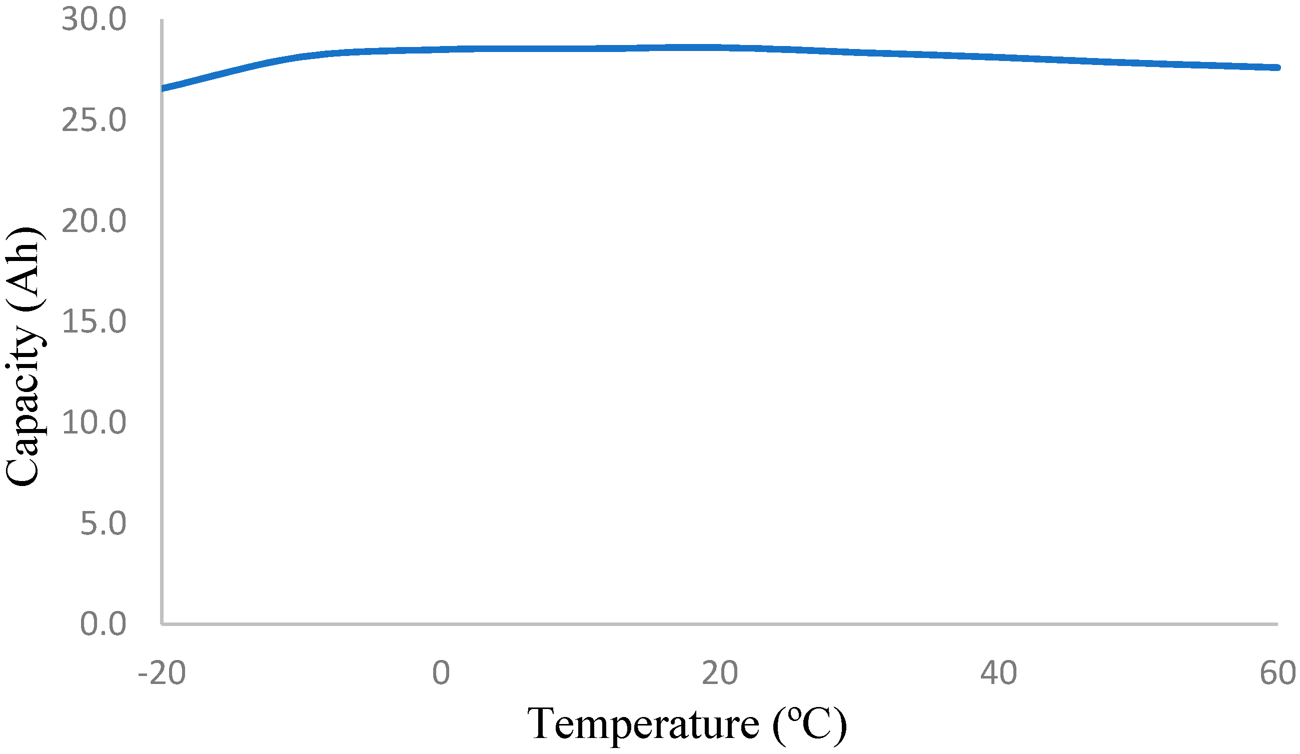
Battery capacity depends on temperature, although the dependence is a function of type and structure of the battery; therefore, for the lithium-ion battery type used for the simulation, we have recovered test results from a previous investigation where we observed that the capacity of the battery remains almost constant for the entire range of the temperature test (Figure 3) [56]

The analysis of the results shown in Figure 3 indicates that the variation of battery capacity in the temperature range from −10 °C to 60 °C is of 3.5%; therefore, we assume that the battery capacity is constant.

Battery capacity is also dependent on the type of discharge rate; for a lithium battery, this dependence has been found [57].

$$C_i=C_n\left(f_i/f_{ref}\right)$$

(21)

C_i represents the real capacity of the battery for a specific discharge rate, while C_n is the nominal capacity at fully charge state. The f-factor is the so-called capacity correction factor, and it is obtained from the following expression [26]:

$$f_i=0.9541{\left(t_i\right)}^{0.0148}$$

(22)

$$f_{ref}=0.9541{\left(t_{ref}\right)}^{0.0148}$$

(23)

where the reference discharge time, t_ref, is currently taken as 20 h, and the discharge time, t_i, can be calculated from the following equation.

$$t_i=\left(C_n/I_i\right)$$

(24)

By combining Equations (20)–(22), we obtain the following.

$$C_i=C_n{\left(I_{ref}/I_i\right)}^{0.0148}$$

(25)

Since a daily trip can be represented as a combination of several segments, each one having specific dynamic conditions, average speed, acceleration and slope of the road, the battery capacity cannot be assumed to have a unique value; therefore, Equation (12) must be applied to every single segment of the daily trip, resulting in the following.

$$C_n{\left(\frac{I_{ref}}{I_i}\right)}^{0.0148}\left[V_o-s{(DOD)}_i\right]=\frac{1}{{\eta }_{PWT}}\left(m{a}_i+k{v}_i^2+\mu mg+mg\sin {\beta }_i\right)<v_i>{\left(\Delta t\right)}_i$$

(26)

By applying Equation (18), we obtain the following.

$$\frac{C_n}{100}{\left(\frac{I_{ref}}{I_i}\right)}^{0.0148}\left(V_o\left[100-{(DOD)}_i\right]+V_{off}{(DOD)}_i\right)=\frac{1}{{\eta }_{PWT}}\left(m{a}_i+k{v}_i^2+\mu mg+mg\sin {\beta }_i\right)<v_i>{\left(\Delta t\right)}_i$$

(27)

In general terms, the mathematical equation for the DOD coefficient can be expressed as follows:

$${\left(DOD\right)}_i=Q_i/C_i=I_i{\left(\Delta t\right)}_i/C_i$$

(28)

where Q_i accounts for the extracted charge from the battery.

Since the discharge process is continuous, the DOD coefficient must be expressed in terms of the cumulative charge extracted from the battery; thus, the following is the case.

$${\left(DOD\right)}_i={\displaystyle \sum _{j=1}^i\frac{Q_j}{C_j}}$$

(29)

By using Equation (25), we obtain the following.

$${\left(DOD\right)}_i=\frac{1}{C_n{\left(I_{ref}\right)}^{0.0148}}{\displaystyle \sum _{j=1}^i{\left(I_j\right)}^{1.0148}{\left(\Delta t\right)}_j}$$

(30)

Now, by replacing in Equation (27), we obtain the following.

$$\frac{1}{100}{\left(\frac{1}{I_i}\right)}^{0.0148}\left[100V_o{C}_n{\left(I_{ref}\right)}^{0.0148}-\left(V_o-V_{off}\right){\displaystyle \sum _{j=1}^i{\left(I_j\right)}^{1.0148}{\left(\Delta t\right)}_j}\right]=\frac{1}{{\eta }_{PWT}}\left(m{a}_i+k{v}_i^2+\mu mg+mg\sin {\beta }_i\right)<v_i>{\left(\Delta t\right)}_i$$

(31)

Equation (31) represents the energy balance at every single segment of a daily trip for the electric vehicle.

7. Electric Vehicle Driving Range

The range of an electric vehicle, based on a daily trip, can be defined as the maximum number of days the electric vehicle can use the battery before recharging is required. By using the expression for daily energy consumption, ξ_day, which is given by the following:

$${\xi }_{day}=\frac{1}{100}{\left(\frac{1}{I_i}\right)}^{0.0148}\left[100V_o{C}_n{\left(I_{ref}\right)}^{0.0148}-\left(V_o-V_{off}\right){\displaystyle \sum _{j=1}^i{\left(I_j\right)}^{1.0148}{\left(\Delta t\right)}_j}\right]\frac{1}{{\eta }_{PWT}}$$

(32)

We can obtain the autonomy from the following equation.

$${{\rm T}}_{aut}=\frac{CV{\eta }_{PWT}}{\frac{1}{100}{\left(\frac{1}{I_i}\right)}^{0.0148}\left[100V_o{C}_n{\left(I_{ref}\right)}^{0.0148}-\left(V_o-V_{off}\right){\displaystyle \sum _{j=1}^i{\left(I_j\right)}^{1.0148}{\left(\Delta t\right)}_j}\right]}$$

(33)

Equation (33) indicates that the lower the powertrain efficiency, the shorter the autonomy.

Nevertheless, the battery capacity and voltages do not remain constant as the discharge process is occurring; therefore, the CV product must be expressed as follows.

$$CV={\displaystyle \sum _{i=1}^n{C}_i{V}_i}={\displaystyle \sum _{i=1}^n\left[C_n{\left(I_{ref}/I_i\right)}^{0.0148}\right]}\left[\frac{V_o\left[100-{\left(DOD\right)}_i\right]+V_{off}{\left(DOD\right)}_i}{100}\right]$$

(34)

By replacing Equation (33), we obtain the following.

$$\begin{array}{l}{\mathsf{{\rm T}}}_{aut}=\frac{{\displaystyle \sum _{i=1}^n\left[C_n{\left(I_{ref}/I_i\right)}^{0.0148}\right]}\left\{V_o\left[100-\frac{1}{C_n{\left(I_{ref}\right)}^{0.0148}}{\displaystyle \sum _{j=1}^i{\left(I_j\right)}^{1.0148}{\left(\Delta t\right)}_j}\right]+V_{off}\frac{1}{C_n{\left(I_{ref}\right)}^{0.0148}}{\displaystyle \sum _{j=1}^i{\left(I_j\right)}^{1.0148}{\left(\Delta t\right)}_j}\right\}}{{\left(\frac{1}{I_i}\right)}^{0.0148}\left[100V_o{C}_n{\left(I_{ref}\right)}^{0.0148}-\left(V_o-V_{off}\right){\displaystyle \sum _{j=1}^i{\left(I_j\right)}^{1.0148}{\left(\Delta t\right)}_j}\right]}{\eta }_{PWT}\\ \end{array}$$

(35)

Equation (32) provides the range of the electric vehicle on a daily trip basis as a function of characteristic parameters of the battery, nominal capacity C_n, reference discharge current I_ref, open circuit voltage V_o and cut-off voltage V_off, as well as a function of the operational parameters, discharge current I_i and time of running, (Δt)_i.

It can be observed that discharge current adopts two forms, I_i and I_j, both corresponding to the same parameter. The difference in the subindex notation corresponds to the cumulative effect when calculating the depth of discharge coefficient, where the discharge current subindex is noted as j in order to distinguish from an individual segment of the discharge for which the subindex is noted as i.

8. Simulation Process

To evaluate the autonomy of an electric vehicle, a simulation process has been developed; the simulation is based on a model that reproduces the performance of the real prototype. To perform this, the characteristics of the electric vehicle as well as of the battery must be known in order to establish the modeling values; these characteristics are, on the side of the vehicle, the mass, the operational voltage of the electric engine, the wheel radius, the model of the vehicle, the type of tires and road type. On the side of the battery, the characteristics include battery energy, nominal capacity, open circuit and cut-off voltage and reference discharge time.

To simulate the performance of the battery, the aforementioned characteristics are essential since they are variables of the mathematical expression that determines the available power and energy of the battery for the specific operational conditions.

Vehicle mass is used to obtain global force while the operational voltage of the electric engine sets up the battery voltage. The wheel radius, combined with the angular speed of the engine, is used to determine the vehicle speed, which is one of the parameters involved in the calculation of the global force; the model of the vehicle determines its shape and size and, thus, the drag coefficient. Finally, the type of tires and road establishes the rolling factor, which also intervenes in the determination of global force.

Vehicle speed and acceleration, below the limits imposed by the manufacturer, are subject to the driver’s decision, which means that they depend on the driving mode. Three different driving modes have been considered: aggressive, moderate or normal and gentle. The three modes are distinguished by the acceleration rate, for which its values are indicated in

Table 1. Acceleration values for the different driving modes.

Driving Mode	Acceleration (m/s2)	t (s) (0–100 km/h)
Aggressive	3.50	6.9
Moderate/Normal	2.50	11.1
Gentle	1.50	18.5

.

The values presented in Table 1 match, within a low margin error, the current values of combustion engine vehicles that are currently commercialized.

The first category with the highest acceleration rate corresponds to luxury and expensive vehicles with very powerful engines but are not accessible to most of the drivers. Moderate or normal acceleration range includes the majority of urban utility vehicles, compact, saloon or SUVs. The gentle acceleration category is devoted for small cars with low power engines and very high mileage rates.

To facilitate the driver’s decision, the simulation will provide the option to users to decide whether or not the default option is chosen. Default option is automatically selected by the control system according to set up parameters that search for optimum performance of the battery service for a specific vehicle and trip. The default option, in our simulation, has been assigned to the moderate/normal acceleration rate. Drivers, however, can enter the advanced mode where the control system allows choosing the acceleration rate that is preferred, thus rearranging the calculation according to the driver’s selection.

The simulation has the goal of reproducing real driving situations based on an urban daily trip. The trip has been divided into five segment categories: normal driving, acceleration and deceleration process and ascending or descending roads. Normal driving has been configured to maintain constant vehicle speed, while acceleration or deceleration processes correspond to segments where the vehicle speed is increasing or decreasing due to the mechanical action on the vehicle’s dynamic state, which means pressing or releasing the accelerator pedal. Ascent and descent segments are those where the slope of the road exceeds a threshold that is either positive or negative.

Drag coefficient and rolling factor are currently set up according to the vehicle mass range; the typical values have been represented in

Table 2. Drag coefficient and rolling factor for EV’s.

Mass (kg)	k	μ
1000–2500	0.578	0.15
3000–3500	1.458	0.15

.

The average vehicle speed is calculated by the classical expression of kinematics, v = d/t, where the travelling distance and the time are retrieved by using the Google Maps application. However, when our software determines the route to be taken, it will not determine all the fractions of the route in the form of the five algorithms. In fact, our software will transcribe the path in the form of the following (Figure 4):

• A horizontal path (which takes into account normal walking, acceleration and deceleration);
• An ascending part;
• A descending part.

The path can then be simplified as represented in the following figure.

It is important to know that there is no access to descent or ascent percentages on Google Maps, and consequently this application does not allow us to obtain all the necessary information; therefore, the Google Maps application will only be used to define the route and to determine the distance and duration of the trip from which we can calculate the average speed.

To determine the inclination of the road, different solutions are possible, but the preferred solution is the inclinometer [58,59,60,61]. This solution will allow obtaining the inclination of the daily route taken by the user in order to determine the final angle of ascent and descent.

In our model, we have chosen this last system because of its major sensitivity to changes in road tilt. The vehicle speed is calculated by using the following expression [62,63]:

$$v=\frac{\pi D\omega r_g}{\left(1000/60\right)}$$

(36)

where D is the wheel diameter, ω the engine rotational speed in rpm and r_g the gear box ratio. These three parameters are currently known from the vehicle manufacturer data sheet.

In the case where the trip segment is made up of up and down sections, we have to group all ascent sections in one as well as another section for the descent; in such a case, the equivalent tilt angle of the road, either with respect to ascent or descent, is given by the following:

$$\beta =\frac{{\displaystyle \sum _{i=1}^n{d}_i{\beta }_i}}{{\displaystyle \sum _{i=1}^n{d}_i}}$$

(37)

where the subindex i corresponds to the number of sections within the segment, and n is the number of sections.

9. Software Development

To simulate the performance of a prototype vehicle under specific driving conditions, it is necessary to develop a software program that reproduces the different steps of daily driving. This program commands a control system that receives information of the variables intervening in the daily driving.

The driver can obtain useful information from his/her daily driving route as follows:

-

The energy spent in percentage (%);

-

The remaining battery charge in percentage (%);

-

The autonomy of the battery and, therefore, of the EV in hours (h).

Moreover, all the data on the power spent for each stage (acceleration, normal driving, deceleration, ascent and slope) will be displayed, as well as the distances traveled at every segment.

The process is described in the following charts (Figure 5 and Figure 6).

Driving mode

The user chooses his/her driving mode, i.e., aggressive, normal or gentle.

According to this mode, the acceleration taken into account in the calculations is different (Table 1). In order to validate his choice, it is necessary to select one of the three proposals. An informative message appears when the user has already selected one of the options.

Percentage in horizontal path (Percentage)

In this second window, the user selects the percentages for acceleration, normal driving and deceleration on a horizontal path. The default values are already set up, but they can be changed depending on the driver’s choice.

If the sum of the percentages is not 100%, a warning message appears, otherwise an OK message shows up. It is necessary for the user to click on the VALIDATE button at the bottom of the tab in order to save the chosen values.

Choice of the path (Google Maps)

The user is directed to Google Maps through an informative page to enter his destination, from which distance and duration of the journey are provided. The user will then have to convert the values in kilometers and minutes on the software in order to make calculations.

As soon as this is performed, it is necessary to click on the CALCULATE button and an information message will appear to inform the user that the calculations have been performed.

Display of characteristic data (Data)

The user should have access to the necessary characteristic values of the battery and the electric vehicle. In other words, we have the following:

-

Percentage of energy dissipated (%);

-

Autonomy (h);

-

Remaining charge in the EV (%).

Characteristics of the pathway

On this tab, the user can check the characteristics of the path. These data are only for the driver’s information.

Simulation data (Simulation)

This tab provides useful information for the simulation with the setup explained in the next main part.

10. Carbon Emissions

Carbon emissions can be direct or indirect; in the case of road transport, indirect emissions are due to the manufacturing process, which in almost 100% of the cases uses fossil fuels. By neglecting these effects because they affect any type of vehicle (whether electric or internal combustion engines), only direct emissions remain.

Direct emissions come from the combustion of fossil fuels or hydrocarbon materials. In the case of road transport, the emissions are produced by the combustion of gasoline and diesel, which are the main energy sources for ICE vehicles.

Many tools have been used to predict the evolution of the CO₂ content in the atmosphere, showing that the predicted threshold for environmental preservation has been surpassed long ago, especially in urban areas.

The avoidance of these types of emissions can be realized by using full electric vehicles (EV) or hybrid, HEV or PHEV. The latter type of electric vehicles only partially remedy CO₂ emissions; therefore, it is out of focus. It is true that in urban traffic the use of hybrid electric vehicles helps to reduce air pollution level, but it does not solve the problem at the necessary rate; therefore, the replacement of ICE vehicles by full electric ones (EV’s) is mandatory if we intend to invert the increasing trend of CO₂ emissions.

To obtain the carbon footprint of a vehicle, the determination of fuel consumption is necessary. Nevertheless, the carbon footprint is different from ICE vehicles to electric vehicles, HEV, PHEV or EV. In the case of ICE vehicles, once the fuel consumption is known, carbon emissions are obtained by using the following expression:

$$m_{{\left(C{O}_2\right)}_g}=2.196kg/l_f$$

(38)

$$m_{{\left(C{O}_2\right)}_d}=2.471kg/l_f$$

(39)

where subindexes g and d account for gasoline and diesel, and l_f is the fuel consumption in liters.

The above expressions should be changed if we express fuel consumption in gallons, which is common in the American market; in such a case, the carbon emissions are given by the following.

$$m_{{\left(C{O}_2\right)}_g}=18.324pounds/gallon$$

(40)

$$m_{{\left(C{O}_2\right)}_d}=20.619pounds/gallon$$

(41)

Hybrid and plug-in electric vehicles generate carbon emissions since they operate partially with an electric engine; however, their emissions are out of focus since the analysis in this paper has been developed only for full electric vehicles.

Based on modelling and simulation of the driving range, we can establish the carbon emissions savings as follows.

$$S_{C{O}_2}=m_{{\left(C{O}_2\right)}_{g,d}}\left(FC\right)\left(DR\right)$$

(42)

The average fuel consumption should be expressed as follows.

$$FC={\displaystyle \sum _{i=1}^n{\left(FC\right)}_i=\frac{1}{\rho {\eta }_{th}CH}{\displaystyle \sum _{i=1}^n{P}_i{t}_i}}$$

(43)

Therefore, the following is the case.

$$S_{C{O}_2}=m_{{\left(C{O}_2\right)}_{g,d}}\frac{DR}{\rho {\eta }_{th}CH}{\displaystyle \sum _{i=1}^n{P}_i{t}_i}$$

(44)

Equation (43) provides an expression to determine the carbon emissions savings as a function of the driving range that can be obtained by applying the proposed model in this paper.

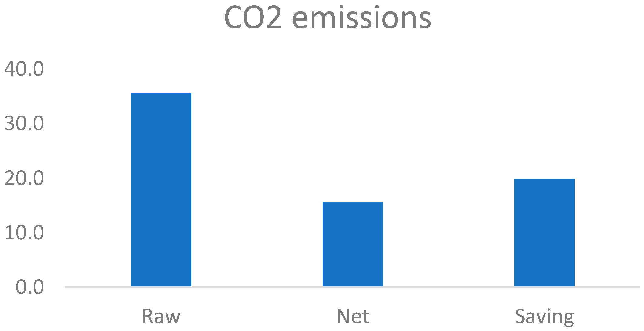
The CO₂ emission savings, due to the use of electric vehicles (EV’s), can be treated under two different points of view: raw saving and net saving. Raw saving is the one generated by avoiding carbon emissions from the exhaust pipe of an ICE vehicle; net saving takes into account emissions due to the electricity generated when recharging the batteries of the electric vehicles.

The calculation of net saving is rather complicated since electricity generation differs from one process to another; in the case where electricity is generated by renewable energy sources such as photovoltaics, wind energy, tidal or waves systems or hydraulic power plants, we can consider that there are no carbon emissions due to electricity generation, at least in terms of direct emissions. On the other hand, if electricity is generated in fossil fuel power plants, there is a carbon footprint that should be taken into consideration.

To determine this footprint, it is necessary to know the type of fuel used, the kind of thermodynamic cycle and the efficiency of the process. Since there are many options, it would be tedious to analyze all cases; however, a standard case can be used as a reference. Neglecting nuclear plants that are currently in sharp decline due to fear of radioactive waste, the most effective method for electricity generation is the combined cycle power plants; these plants use gas as fuel to generate electricity in a gas turbine and water vapor in a secondary vapor turbine. Since water vapor is generated through heat recovering from the enthalpy of the released gas at the gas turbine, only the gas used in the primary section produces carbon emissions.

According to the literature [64], natural gas emits around 204 g (CO₂)/kWh_t. Considering an average efficiency of 70% in the combined cycle, which is a realistic value, the net CO₂ emissions is 291.4 g (CO₂)/kWh_e. On the other hand, in order to recharge electric vehicles, electricity must be carried from the power plant to the recharging point, a process that generates energy losses. Although the energy loss coefficient depends on different factors, we can assume a 1%−2% loss associated with transportation and 5−6% loss with respect to distribution [65]; therefore, a global 7% loss, on average, represents the power loss coefficient.

The carbon mass emissions are obtained from the following.

$$M_{C{O}_2}=m_{{\left(C{O}_2\right)}_g}(FC)(DR)/100$$

(45)

Using values from the simulation, we obtain the following.

$$M_{C{O}_2}=(2.196)(5.7)(284.5)/100=35575.2g$$

(46)

This result corresponds to raw CO₂ emissions saving. The value has been obtained for the aggressive mode, but it is the same for the other two modes since the driving distance remains constant.

The associated emissions with respect to the required electricity generation for recharging the battery of the electric vehicle are calculated by using the following equation:

$$M_{{}_{C{O}_2}}^{el}=\frac{m_{{}_{\left(C{O}_2\right)}}^g{C}_{bat}}{{\eta }_{PW}f}$$

(47)

where C_bat is the capacity that equips the electric vehicle.

Applying the aforementioned values to the CO₂ emissions, we obtain the following.

$$M_{{}_{C{O}_2}}^{el}=\frac{(204)(50)}{(0.7)(0.93)}=15668.2g$$

(48)

The net CO₂ emissions saving is, therefore, described as follows.

$$\Delta M_{C{O}_2}=M_{C{O}_2}-M_{{}_{C{O}_2}}^{el}=35575.2-15668.2=19907g$$

(49)

This represents a reduction of 56%.

The simulation results can be seen in Figure 7.

11. Comparative Analysis

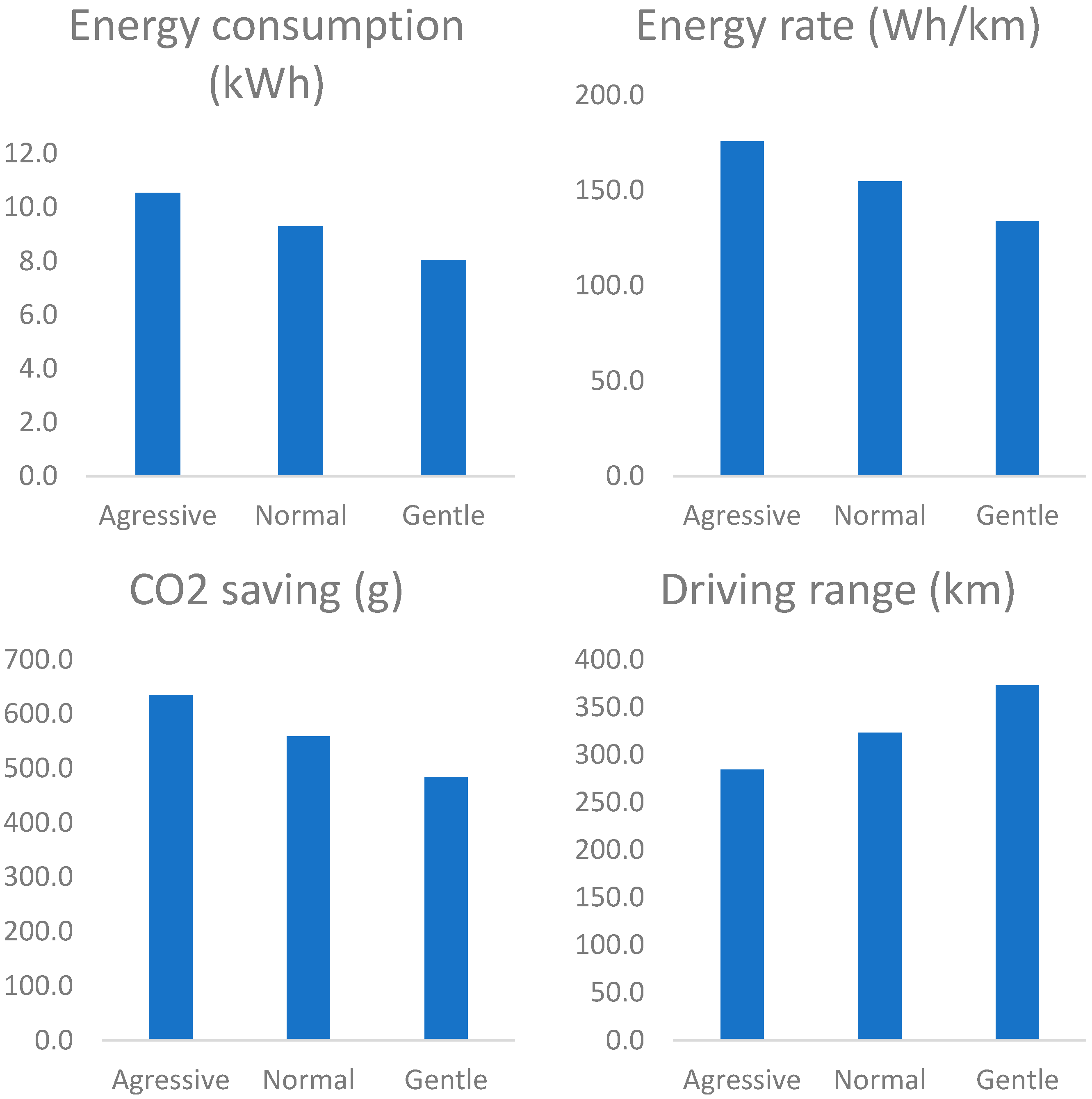
The method of driving influences energy consumption since acceleration depends on it. To show how the type of driving modifies the driving range, we have to consider specific driving and vehicle conditions, with the only difference being the acceleration value. For a standard electric vehicle of 1500 kg of mass equipped with a battery of 50 kWh, driving for a distance of 15 km at an average speed of 60 km/h with a maximum ascent or descent tilt of 3%, we obtain the following results for the three types of driving (Figure 5).

The analysis of the numerical results indicates that there is a reduction of about 30% in the energy consumption, energy rate and CO₂ emissions saving when selecting the aggressive mode compared to the gentle one. The driving range is reduced at 24% if the aggressive mode is selected.

Figure 8 shows a graph representation of the energy consumption, energy rate, CO₂ saving and driving range from the simulation process.

12. Conclusions

A new method to determine an electric vehicle range has been proposed. The method uses online real driving conditions in order to improve the accuracy of the predictions. The protocol software is based on the type of driving modes and on road characteristics.

Driving modes have been associated with an acceleration value, representing most current habits of today’s drivers, but other values can be implemented in the software. The protocol software is adaptive since most of the involved parameters can be updated at the user’s will.

The influence of the variation of battery capacity with discharge rate has been considered for the calculation of available energy; since driving conditions define discharge rate, the calculation of battery power and energy are adjusted with respect to the real situation.

The model predicts a severe reduction in driving range, up to 30%, when operating in the aggressive mode compared to the gentle one. This reduction is of 15% if the normal driving mode is used.

Driving range has been found to be consistent with current values for standard electric vehicles operating in urban routes for a battery specific capacity of 50 kWh. The minimum driving range produced by the simulation is 284.5 km for the aggressive mode, while the maximum driving range of 373.2 km is obtained for the gentle mode.

The new method allows accurate predictions of electric vehicle range as well as the remaining charge in the battery at the end of a daily trip, thus warning the user the need for battery recharge based on predictions of the energy required for the next day trip.

The proposed methodology improves the existing methods since it takes into account real online values of parameters involved in the calculation, thus rendering the calculation of the electric vehicle driving range more accurate. It also can be applied to any driving conditions or driving mode, rendering the model more reliable.

Real fuel consumption is obtained by using the proposed expression that takes real driving conditions into account. Carbon emission savings can also be determined from the estimated driving range by applying the proposed model.

The values obtained for the energy rate throughout the simulation are comparable to those of standard electric vehicles operating today; the values are in the range from 134 Wh/km for the gentle mode to 175.8 Wh/km for the aggressive mode.

A simulation for the CO₂ emissions has been developed, showing a significant reduction by the use of EVs instead of ICE cars. The reduction has been estimated at 56%.