Oil Friction Loss Evaluation of Oil-Immersed Cooling In-Wheel Motor Based on Improved Analytical Method and VOF Model

Abstract

Oil-immersed cooling provides an effective cooling scheme for high-power hub motors with compact structure and serious heating problems. However, with this cooling method, some oil friction loss will be generated, making the output torque and efficiency of the motor lower, which limits its application in the motor. It is essential to get an exact calculation of the oil friction loss so that it can be reduced in the future research. Firstly, a new method was proposed to improve the accuracy of oil friction loss calculated by an existing analytical method (Kori’s method), while the influence laws of oil-soaked depth and rotation speed on it were explored. Secondly, a three-dimensional transient Computational Fluid Dynamic (CFD) model based on Volume of Fluid (VOF) was established, considering the actual complex structure and the disorderly mixing of oil and air inside the motor. Finally, the oil friction loss calculated with an improved analytical method and a VOF model was verified by a testing. It was indicated that the VOF model was more precise but more time-consuming. The proposed method has the second highest accuracy but takes less time.

1. Introduction

An in-wheel motor is the development trend of electric vehicles, towards the trend of high power, large torque, and small volume [1,2,3]. However, the serious heating problem caused by the increase of power density is bound to bring the risk of temperature rise of the motor beyond the safe operation range. Directly oil cooling is one of the solutions, owing to the better cooling effect [4,5,6]. It could contact heating parts with cooling oil to take away heat, overcoming the “Motor Heat Island Effect” of conventional cooling methods such as air cooling [7] and water cooling [8], making heat dissipation more uniform. Directly oil cooling includes oil spray cooling and oil-immersed cooling, both of which have good cooling performance. The oil spray cooling overcomes the flow loss pressure drop in the oil circuit by pressurizing through the oil pump, and then jets the cooling oil to the end of the winding through the oil injection nozzle, so the winding is cooled.

Various studies have been conducted on the thermal performance of the oil-spraying cooling. Ye et al. [9] reformed a motor cooled only by water into one cooled by both water and oil. The cooling oil was injected directly to the end winding through the nozzle which is fixed in the end cover. The temperature rise of the motor was obviously decreased by 40–50%. Tanguy [10] experimentally investigated factors on thermal performance of the oil-spraying cooling motor, including different injector nozzles and the oil flow rate, etc. In order to improve the heat transfer, the dripping injector and a higher flow rate were recommended. The cooling effect of these studies is satisfactory and can greatly reduce the temperature rise of the motor, with nearly no oil friction loss due to rotor rotation. However, there is a disadvantage in the oil-spraying cooling hub motor. Water cooling is used when the matching inverter power is large. Thus, the electric drive system requires two independent cooling systems. The water-cooling system needs water pipes, water pumps, heat exchangers, etc. The oil cooling system also requires oil pipes, oil pumps, oil cooler, etc. This entails increasing parts cost and installation space. In addition, the oil-spraying cooling approach exhibits another drawback of heat dissipation with the existence of some dead zones, such as winding coils in the slots, magnets, where the cooling oil cannot be touched.

The oil-immersed cooling is more suitable for in-wheel motors integrated with reducers and inverters [11]. In this cooling scheme, a certain amount of cooling oil is directly sealed inside the motor, exchanging heat with water used to cool the inverter beforehand. The installation space and cost are greatly saved because some devices reduce. Although the rotor rotation improves the heat transferability, oil friction loss occurs between the rotor and the cooling oil, which not only cuts down the output torque and efficiency of the motor, but also makes it difficult to calculate accurately the temperature increase. Hence, the accurate calculation of oil friction loss is significant to evaluate the performance of the motor and further optimize the design, so that the application of the oil-immersed cooling motor can be popularized in the electric vehicle.

At present, there are some reports about the oil friction loss of an oil-immersed cooling motor, most of those are the analytical method. Montonen [12] presented thermal analyses of a partial oil-immersed cooling Permanent Magnet Synchronous Motor (PMSM). The error of oil friction loss between the calculation using the formulas derived from the gear pair power loss model [13] and measurement was nearly 50%. Ponomarev [14], based on some laws of fluid mechanics, deduced the calculation formula of oil friction loss in a hydraulic motor pump, whereas it can only be used to calculate the loss generated at the air gap, ignoring the loss generated on both sides of the rotor. The same method as Ponomarev was utilized to obtain the oil friction loss at the air gap by Kori and Sugimoto [11], while the loss on both sides of the motor is expressed by an empirical equation. Thus, the error of oil friction loss between the calculation and measurement was down to about 30% at maximum.

In addition, due to the existence of two-phase medium (oil and air) inside the motor, the Volume of Fluid (VOF) model in CFD is often used to evaluate thermal characteristics of directly oil cooling motors [15]. Park [16] established a fluid VOF model for an oil-cooled hollow shaft structure, studied the motion law of oil inside the motor, and elucidated the cooling effect. Nevertheless, the studies on the oil friction loss obtained by VOF model of CFD have not been reported. Therefore, based on the theoretical derivation of Kori [11], an improved analytical method was developed for calculating oil friction loss in this present work. Then, a VOF model of a 200 kW oil-immersed cooling in-wheel motor was built, to truly reflect the actual stirring flow field of the cooling oil. A relevant testing of oil friction loss is carried out in the end.

2. Methods

2.1. An Improved Analytical Derivation

The key to calculate the oil friction loss is to obtain the oil velocity field inside the motor, which is usually obtained by solving the Navier–Stokes equations. The equation is a nonlinear partial differential one with multivariate, so it is very difficult to solve directly. Considering the particularity of each solution to be solved, the following assumptions must be made for the flow of cooling oil under the action of rotor rotation:

(1)

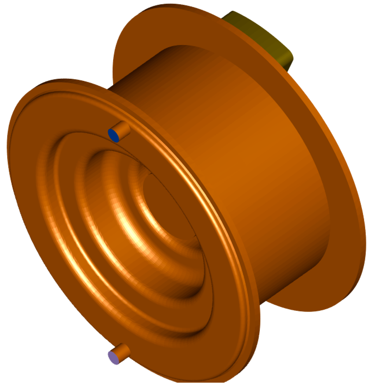
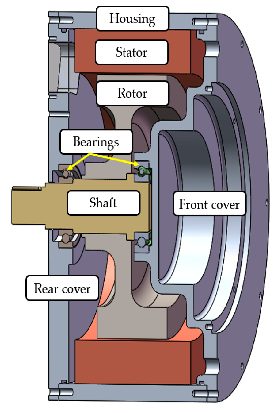
The rotor and stator are both simplified to cylinders, as shown in Figure 1. The oil friction loss is divided into two parts: oil friction loss generated in air gap and oil friction loss generated at both ends of the bottom of the cylinder, which are calculated respectively.

(2)

The fluid motion in the air gap is considered as circular steady laminar flow, so the axial and radial velocities are approximately 0. The mass force is ignored, and there is no pressure difference in the axial direction.

(3)

The fluid flow at the end of the cylinder is assumed to be a steady flow, the velocity does not change with θ, and the mass force is ignored.

The motion of the oil inside the motor can be regarded as the incompressible flows. Each fluid micelle in the oil satisfies the Navier–Stokes Equations of viscous fluid (under cylindrical coordinates):

$$\{\begin{array}{l}\frac{\partial {\upsilon }_r}{\partial t}+{\upsilon }_r\frac{\partial {\upsilon }_r}{\partial r}+\frac{{\upsilon }_{\theta }}{r}\frac{\partial {\upsilon }_r}{\partial \theta }-\frac{{\upsilon }_{\theta }^2}{r}+{\upsilon }_z\frac{\partial {\upsilon }_r}{\partial z}=f_r-\frac{1}{\rho }\frac{\partial p}{\partial r}+\nu (\frac{{\partial }^2{\upsilon }_r}{\partial r^2}+\frac{1}{r}\frac{\partial {\upsilon }_r}{\partial r}-\frac{{\upsilon }_r}{r^2}+\frac{1}{r^2}\frac{{\partial }^2{\upsilon }_r}{\partial {\theta }^2}-\frac{2}{r^2}\frac{{\partial }^2{\upsilon }_{\theta }}{\partial \theta }+\frac{{\partial }^2{\upsilon }_r}{\partial z^2})\\ \frac{\partial {\upsilon }_{\theta }}{\partial t}+{\upsilon }_r\frac{\partial {\upsilon }_{\theta }}{\partial r}+\frac{{\upsilon }_{\theta }}{r}\frac{\partial {\upsilon }_{\theta }}{\partial \theta }-\frac{{\upsilon }_r{\upsilon }_{\theta }}{r}+{\upsilon }_z\frac{\partial {\upsilon }_{\theta }}{\partial z}=f_{\theta }-\frac{1}{\rho r}\frac{\partial p}{\partial \theta }+\nu (\frac{{\partial }^2{\upsilon }_{\theta }}{\partial r^2}+\frac{1}{r}\frac{\partial {\upsilon }_{\theta }}{\partial r}-\frac{{\upsilon }_{\theta }}{r^2}+\frac{1}{r^2}\frac{{\partial }^2{\upsilon }_{\theta }}{\partial {\theta }^2}-\frac{2}{r^2}\frac{{\partial }^2{\upsilon }_{\theta }}{\partial \theta }+\frac{{\partial }^2{\upsilon }_{\theta }}{\partial z^2})\\ \frac{\partial {\upsilon }_z}{\partial t}+{\upsilon }_r\frac{\partial {\upsilon }_z}{\partial r}+\frac{{\upsilon }_{\theta }}{r}\frac{\partial {\upsilon }_z}{\partial \theta }+{\upsilon }_z\frac{\partial {\upsilon }_z}{\partial z}=f_z-\frac{1}{\rho }\frac{\partial p}{\partial z}+\nu (\frac{{\partial }^2{\upsilon }_z}{\partial r^2}+\frac{1}{r}\frac{\partial {\upsilon }_z}{\partial r}+\frac{1}{r^2}\frac{{\partial }^2{\upsilon }_z}{\partial {\theta }^2}+\frac{{\partial }^2{\upsilon }_z}{\partial z^2})\end{array}$$

(1)

Meanwhile, the continuity equation is satisfied as follows:

$$\frac{\partial {\upsilon }_r}{\partial r}+\frac{{\upsilon }_r}{r}+\frac{1}{r}\frac{\partial {\upsilon }_{\theta }}{\partial \theta }+\frac{\partial {\upsilon }_z}{\partial z}=0$$

(2)

where ${\upsilon }_r$,${\upsilon }_{\theta }$,${\upsilon }_z$ are the components of the velocity vector $\upsilon (r, \theta , z)$ of the fluid in three directions.$f_r$, $f_{\theta }$, $f_z$ are the components of the unit mass force vector $f(r, \theta , z)$ of the fluid in three directions. $p$ is the pressure in fluid field. $\nu$ is the kinematic viscosity. $\rho$ is fluid density.

Based on assumptions (1) and (2), it can be concluded that the oil friction loss at the air gap should meet the following requirements:

$$\{\begin{array}{l}{\upsilon }_r={\upsilon }_z=0, {\upsilon }_{\theta }={\upsilon }_{\theta }(r)\\ \frac{\partial }{\partial t}=0, \frac{\partial }{\partial \theta }=0\\ f_r=f_{\theta }=f_z=0, P=P(r)\\ \rho =const\end{array}$$

(3)

Substituting Equation (3) into Equation (2) and Equation (1) can obtain:

$$\{\begin{array}{l}-\frac{{\upsilon }_{\theta }^2}{r}=-\frac{1}{\rho }\frac{dP}{dr}\\ 0=\rho \nu \left[\frac{1}{r}\frac{d}{dr}\left(r\frac{d{\upsilon }_{\theta }}{dr}\right)-\frac{{\upsilon }_{\theta }}{r^2}\right]\end{array}$$

(4)

Equation (4) is a second-order nonhomogeneous differential equation, and its solution is as follows:

$${\upsilon }_{\theta }(r)=C_1\frac{r}{2}+\frac{C_2}{r}$$

(5)

where C₁, C₂ is the undetermined coefficient, which can be solved by the following boundary conditions:

$$\{\begin{array}{l}r=R_o, {\upsilon }_{\theta }=\omega R_o\\ r=R_s, {\upsilon }_{\theta }=0\end{array}$$

(6)

where $R_o$,$R_s$ are the outer diameter of the rotor and the inner diameter of the stator respectively, so the velocity field at the air gap is as follows:

$${\upsilon }_{\theta }(r)=\frac{\omega R_o^2}{R_s^2-R_o^2}\left(\frac{R_s^2}{r}-r\right)$$

(7)

Equation (7) describes the motion law of oil inside the motor, which is also one of the improvements made in this paper compared with Kori’s method [11]. It indicates that the velocity distribution of oil in the air gap is nonlinear. The shear stress on the outer surface of the rotor is obtained according to the generalized Newton’s law of internal friction:

$${\tau }_{\theta r|r=R_o}=-\rho \nu r\frac{\partial }{\partial r}\left(\frac{{\upsilon }_{\theta }}{r}\right)|{}_{r=R_o}=\frac{2\rho \nu \omega R_s^2}{R_s^2-R_o^2}$$

(8)

By surface integration on the outer surface of the rotor, the oil friction loss at the air gap can be obtained as:

$$P_{gap}={\displaystyle \underset{s}{\int }{\tau }_{\theta r}}ds=\frac{4\rho \nu \pi L{R}_s^2{R}_o^2{\omega }^2}{R_s^2-R_o^2}$$

(9)

where L is the axial length of the rotor.

Furthermore, based on assumptions (1) and (3), for the oil friction loss at the end, Equations (1) and (2) can be simplified as:

$$\{\begin{array}{l}{\upsilon }_r\frac{\partial {\upsilon }_r}{\partial r}+{\upsilon }_z\frac{\partial {\upsilon }_r}{\partial z}-\frac{{\upsilon }_{\theta }^2}{r}=-\frac{1}{\rho }\frac{\partial p}{\partial r}+\nu (\frac{{\partial }^2{\upsilon }_r}{\partial r^2}+\frac{1}{r}\frac{\partial {\upsilon }_r}{\partial r}+\frac{{\partial }^2{\upsilon }_r}{\partial z^2})\\ {\upsilon }_r\frac{\partial {\upsilon }_{\theta }}{\partial r}-\frac{{\upsilon }_r{\upsilon }_{\theta }}{r}+{\upsilon }_z\frac{\partial {\upsilon }_{\theta }}{\partial z}=\nu (\frac{{\partial }^2{\upsilon }_{\theta }}{\partial r^2}+\frac{1}{r}\frac{\partial {\upsilon }_{\theta }}{\partial r}+\frac{{\partial }^2{\upsilon }_{\theta }}{\partial z^2})\\ {\upsilon }_r\frac{\partial {\upsilon }_z}{\partial r}+{\upsilon }_z\frac{\partial {\upsilon }_z}{\partial z}=-\frac{1}{\rho }\frac{\partial p}{\partial z}+\nu (\frac{{\partial }^2{\upsilon }_z}{\partial r^2}+\frac{1}{r}\frac{\partial {\upsilon }_z}{\partial r}+\frac{{\partial }^2{\upsilon }_z}{\partial z^2})\\ \frac{\partial {\upsilon }_r}{\partial r}+\frac{{\upsilon }_r}{r}+\frac{\partial {\upsilon }_z}{\partial z}=0\end{array}$$

(10)

where ${\upsilon }_r(\omega , \nu , z, r)$,${\upsilon }_{\theta }(\omega , \nu , z, r)$,${\upsilon }_z(\omega , \nu , z, r)$, and $p(\omega , \nu , z, r)$ are respectively functions of speed $\omega$, kinematic viscosity $\nu$, axial length $z$, and arbitrary radius $r$. We can obtain that ${\upsilon }_z$ is independent of $r$, supposing that ${\upsilon }_r$ and ${\upsilon }_{\theta }$ are proportional to $r$ under centrifugal force. The $\pi$ theorem is used to convert a function with four independent variables into a function with only one dimensionless variable $\xi (z^{*})$, $\phi (z^{*})$, $\kappa (z^{*})$, $P(z^{*})$ the non-dimensional variable $z^{*}=z\sqrt{\omega /\nu }$, and satisfies:

$$\{\begin{array}{l}{\xi }^2+{\xi }^{\prime }\kappa -{\xi }^{″}-{\phi }^2=0\\ 2\xi \phi +\kappa {\phi }^{\prime }+{\phi }^{″}=0\\ P^{\prime }+\kappa {\kappa }^{\prime }-{\kappa }^{″}=0\\ 2\xi +{\kappa }^{\prime }=0\end{array}$$

(11)

$$\{\begin{array}{l}{z}^{*}=0, \xi =0, \kappa =0, \phi =1, P=0\\ z^{*}=\infty , \xi =0, \phi =0\end{array}$$

(12)

Although the multivariable partial differential equation in Equation (10) is simplified into the above constant coefficient differential equation in Equation (11), it is still difficult to solve it directly, and numerical integration method can be used to solve it under the boundary conditions in Equation (12).

Thus, the shear stress of the rotor end face is:

$${\tau }_{z\theta |z=0}=\rho \nu \frac{\partial {\nu }_{\theta }}{\partial z}|{}_{z=0}=0.616\rho \sqrt{\nu {\omega }^3}r$$

(13)

The surface integral of the rotor end face with a radius can be used to obtain the oil friction loss at the end face. This is the second improvement compared with Kori’s method [11], and it corrects the relationship between the loss and the speed and viscosity:

$$P_{end}=2\omega {\displaystyle \underset{s}{\int }{\tau }_{z\theta |z=0}ds=}0.616\pi \rho \sqrt{\nu {\omega }^5}{R}_o^4$$

(14)

When the rotor is partly soaked in the cooling oil, the oil-soaked depth is assumed to be h, as shown in Figure 1. The air gap coefficient $k_{h\_gap}$ and end face coefficient $k_{h\_end}$ are used to consider the effect of partial oil immersion, which are obtained by Equation (15):

$$\{\begin{array}{l}{k}_{h\_gap}=2\theta /2\pi ={\cos }^{-1}((H-h)/R_o)/\pi \\ k_{h\_end}={\cos }^{-1}((H-h)/R_o)/\pi -0.5\sin \left[2{\cos }^{-1}((H-h)/R_o)\right]/\pi \end{array}$$

(15)

Thus, the loss of oil friction $P_f$ can be as follows:

$$P_f=P_{gap}\times k_{h\_gap}+P_{end}\times k_{h\_end}$$

(16)

2.2. Numerical Analysis Procedure

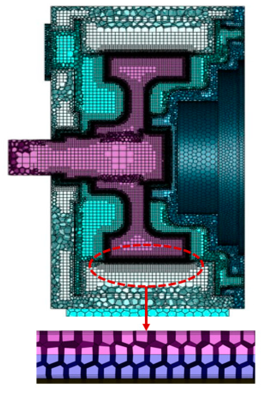
2.2.1. Model Definition and Mesh

The main parameters of the in-wheel motor used in this paper are shown in

Table 1. Parameters of in-wheel motor.

Parameter	Value
Rated power/kW	200
Peak power/kW	445
Rated power/rpm	1000
Maximum speed/rpm	5000
Slots	36
Stator Diameter/mm	430
Air gap/mm	2
Rotor Diameter/mm	316
Axial length of iron core/mm	104
inner cavity volume/mL	8300

. The coolant greatly affects cooling performance, and the automatic transmission fluid (ATF) oil is used because of its excellent insulation performance, low value of viscosity, and high thermal conductivity, which meet the insulation and lubrication technical requirements of an oil cooling type electric vehicle motor [17]. The material properties of oil and air are shown in

Table 2. Parameters of oil and air at 20 centigrade under standard atmospheric pressure.

Medium	Density (kg/m3)	Dynamic Viscosity (Pa × s)
Oil-ATF220	867.2	0.07805
air	1.205	1.81 × 10−5

.

A three-dimensional geometric model of a 200kW hub motor was established, as shown in Figure 2. The structural components include stator, rotor, shaft, housing, and covers. To save the calculation cost, the stator with windings was simplified into a regular cylinder. Since this motor was a surface PMSM, the pole arc coefficient was 0.972, close to 1, and the permanent magnet was fixed radial by 0.8 mm thick carbon fiber circular sheath, fluid disturbance caused by circumferential clearance between each pole could be ignored. In such condition, the permanent magnet, rotor, and sheath were combined together.

The internal space of the motor was extracted into a fluid domain, as shown in Figure 3, which includes cooling oil and air. Poly-hexahedron elements were employed to create a 3D mesh with a minimum size set at 1 mm, as shown in Figure 4, the number of volume cells is 4.85 million, and the maximum skewness is less than 0.57, which indicates that the element quality is fine.

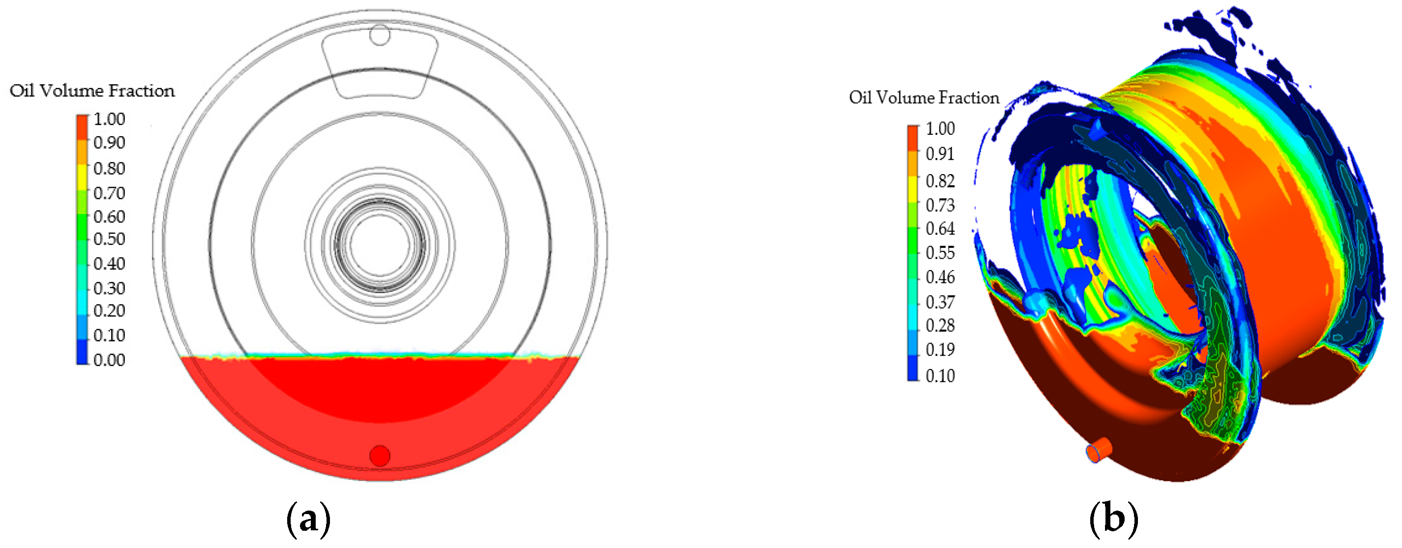
2.2.2. Governing Equation

When the oil-immersed cooling is used, the flow inside the motor involves two phases: oil and air. It is an unsteady Gas-Liquid Cocurrent Flow problem that the oil and air mix in disorder and their interfaces change with time during the motor rotation. The VOF model was used to track the interface between two incompatible phases by a volume fraction $\alpha$. For the oil-air two-phase flow problem, its density $\rho$, dynamic viscosity μ, and volume fraction $\alpha$ satisfy the following relations:

$$\rho ={\alpha }_{oil}{\rho }_{oil}+{\alpha }_{air}{\rho }_{air}$$

(17)

$$\mu ={\alpha }_{oil}{\mu }_{oil}+{\alpha }_{air}{\mu }_{air}$$

(18)

$${\alpha }_{oil}+{\alpha }_{air}=1$$

(19)

In addition, the continuity and momentum equations also need to be followed.

Continuity equation in a mixture:

$$\frac{\partial \rho }{\partial t}+\nabla \cdot \left(\rho \stackrel{\rightharpoonup }{u}\right)=0$$

(20)

Momentum equation in a mixture:

$$\frac{\partial }{\partial t}\left(\rho \stackrel{\rightharpoonup }{u}\right)+\nabla \cdot \left(\rho \stackrel{\rightharpoonup }{u}\stackrel{\rightharpoonup }{u}\right)-\nabla p-\rho \stackrel{\rightharpoonup }{F}=0$$

(21)

where $\stackrel{\rightharpoonup }{u}$ is a velocity vector, $\frac{\partial }{\partial t}\left(\rho \stackrel{\rightharpoonup }{u}\right)+\nabla \cdot \left(\rho \stackrel{\rightharpoonup }{u}\stackrel{\rightharpoonup }{u}\right)$ is the inertial forces per unit volume, $\nabla p$ represents divergence of stress tensor per unit volume, and $\rho \stackrel{\rightharpoonup }{F}$ is the mass force per unit volume.

2.2.3. Sliding Mesh Method and Boundary Conditions

The modeling of rotation in CFD is crucial due to the strong effects of rotation on the internal flow in the oil-immersed cooling motors. The sliding mesh method is used to model flows where the shape of the domain is changing with time due to motion on the domain boundaries. It is useful to solve the unsteady Gas-Liquid Cocurrent Flow problem. Consequently, an interface boundary between the rotation fluid and static fluid domain is necessary. In addition, the boundary near the wall is set to Wall.

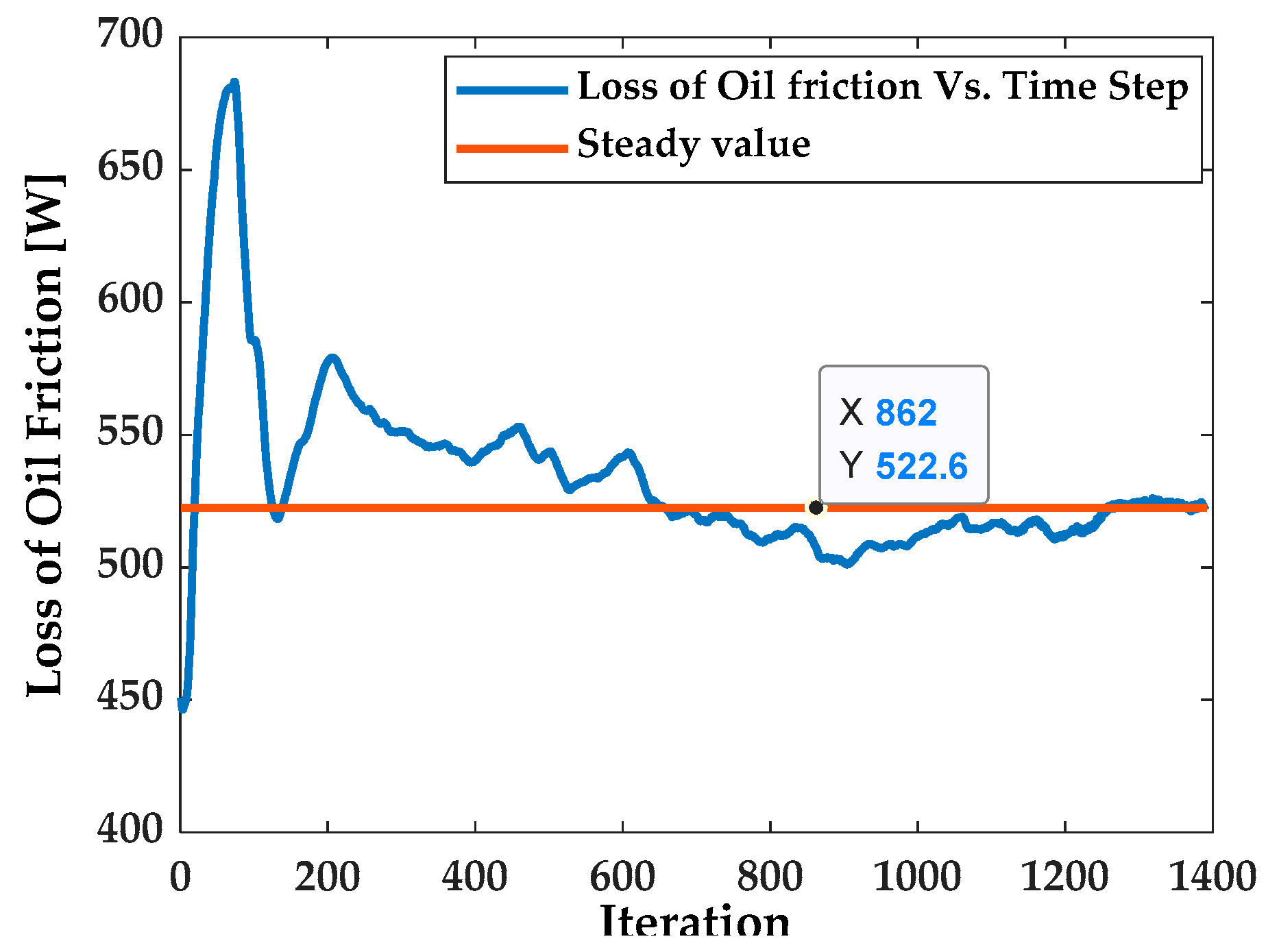
2.2.4. Convergence Criteria

The convergence criteria in CFD are often judged by the residual. The residual is a measure of the local imbalance of each conservative control volume equation. It is the most important measure of convergence as it relates directly to whether the equations have been solved accurately. In this study, the residual value of some quantities, such as the continuity, the velocity, the volume of fluid, etc., is suggested to be set 1 × 10⁻⁵,which is good convergence, as given by the Fluent help manual.

2.3. Experimental Procedure

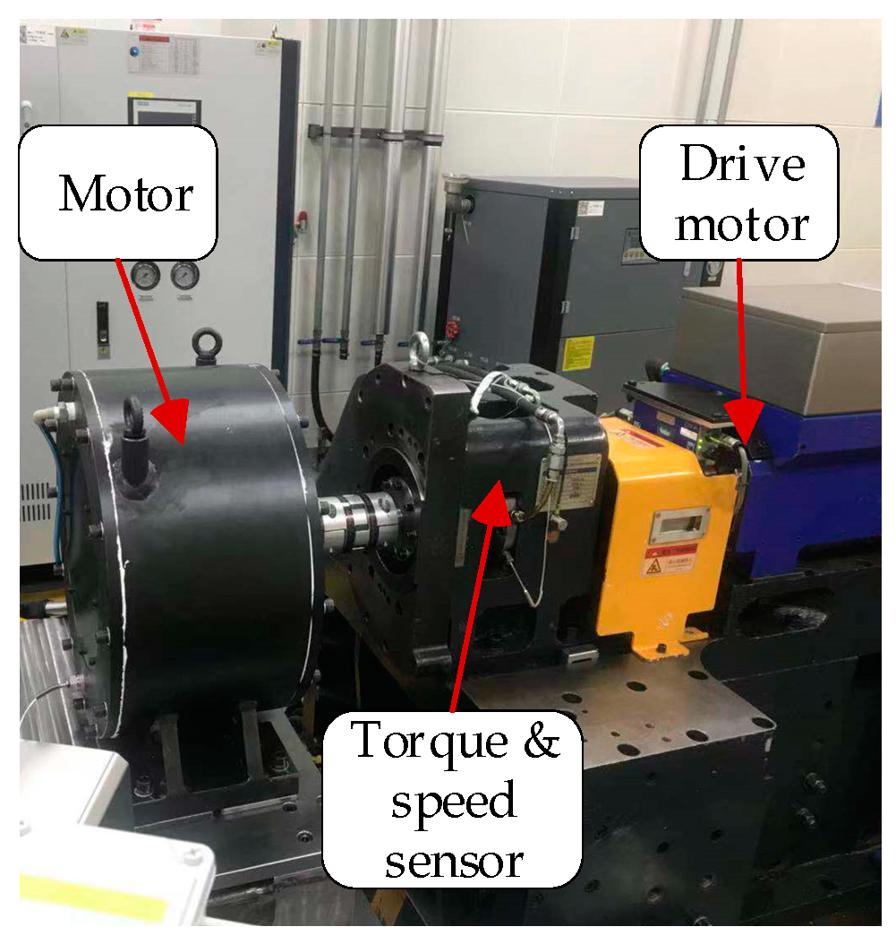
2.3.1. Setup

To verify the effectiveness of the improved analytical formula in Section 2.1 and the accuracy of the VOF numerical model established in Section 2.2, which takes the mixing effect of oil and air into account, a testing of oil friction loss was designed, as shown in Figure 5. The measuring cup was used to accurately take a certain amount of oil. The drive motor was used to change the rotation speed, which can allow the shaft to rotate at up to 12,000 rpm. The torque and speed sensor were used to test the mechanical loss of the motor with or without oil inside. All the measurements are carried out in an open circuit.

2.3.2. Loss Measurement

The oil friction loss can be obtained by formula (22), where $P_{oilfriction}$ is the oil friction loss, $\omega$ is the electric motor speed, $T_{shaft}$ is the electric motor torque, $T_{oilfriction}$ is the torque resulting from the oil friction, and $T_{mech}$ is the torque resulting from the mechanical friction, including air friction, bearing friction:

$$P_{oilfriction}=\omega T_{oilfriction}=\omega (T_{shaft}-T_{mech})$$

(22)

Therefore, the detailed test procedure is as follows:

Test the loss without oil inside the motor. Set the speed of the drive motor to 1000 rpm, and drag the testing motor rotating together. Record the torque while the measured data being stable. Then, change the speed and operate repeatedly.

(1)

Test the loss with a fixed oil-soaked depth inside the motor. Pour 1500 mL of ATF cooling oil into the testing motor, which is equivalent to the oil-soaked depth of 112.5 mm. The equivalent method can be followed as formula (23), which is obtained by numerical fitting of the fifth-degree polynomial. Record the stable torque with different speeds.

(2)

Testing the loss with different oil-soaked depths. Set a fixed speed of 1000 rpm, pour 800 mL of ATF cooling oil into the testing motor firstly, and record the stable torque. Then, change the oil quantity and record the stable torque:

$$h=0.2713\times V^5-2.963\times V^4+14.6\times V^3-39.64\times V^2+88.53\times V+32.51$$

(23)

where $h$ is the oil-soaked depth whose unit is mm, and $V$ is the volume of the cooling oil whose unit is L.

2.3.3. Uncertainly Analysis

The uncertainty of the torque measurement can be represented in equation form as follows:

$$u(T)=\sqrt{{[u(T_t)]}^2+{[u(T_0)]}^2}$$

(24)

where the uncertainty in the torque transducers $u(T_t)$ is less than 0.002 Nm; and the $u(T_0)$ is the torque transducer offset. Finally, the uncertainty of the measured torque is 0.0076 Nm at low speeds and 0.0050 Nm at high speeds.

3. Results

The improved analytical formula of the oil friction loss in Section 2.1 is as follows:

$$P_f=\frac{4\rho \nu L{R}_s^2{R}_o^2{\omega }^2{\cos }^{-1}((H-h)/R_o)}{R_s^2-R_o^2}+0.616\rho \sqrt{\nu {\omega }^3}{R}_o^4\left\{{\cos }^{-1}((H-h)/R_o)-0.5\sin \left[2{\cos }^{-1}((H-h)/R_o)\right]\right\}$$

(25)

It could be seen that the oil friction loss is affected by some physical parameters of the cooling oil and the structural sizes of the motor. In view of these factors, reasonable selection of cooling oil and optimization design of motor structure are of great significance to reduce the loss.

Six hours later, the simulation was done. Figure 6 shows the oil distribution at oil-soaked depth h = 0.1125 m. Figure 6a shows the oil distribution when the rotor is still, and Figure 6b shows the oil distribution when the damping torque generated by oil stirring is stable at rotation speed n = 1000 rpm. It can be seen that the oil rotates with rotor, and some oil is thrown up and splashed to the end of the stator winding.

Figure 7 shows the velocity field of oil inside the motor when the flow state of oil gets steady at rotation speed n = 1000 rpm and oil-soaked depth h = 0.1125 m. It can be seen that the velocity of the oil close to the wall is 0, and the oil in the rotor rotation region has the maximum velocity and moves together with the rotor, which indicates the applicability of the VOF model for solving such problems. After 1400 iterations, the loss of oil friction gradually converges to 522.6 W, as shown in Figure 8.

Figure 9 shows the comparison between the calculation with three methods and testing values of the oil friction loss. Figure 9a shows the relationship between the loss and the oil-soaked depth at a rotation speed of 1000 rpm. Both calculation and measurement indicate that oil friction loss is proportional to the depth of oil soaked inside the motor. Figure 9b shows the relationship between the loss and the rotating speed when the oil-soaked depth h is 0.1125 m, which points out that oil friction loss increases exponentially with the rotation speed.

In addition, the values calculated by the improved analytical method are closer to the experimental value than Kori’s method, but worse than the VOF numerical model. Furthermore, the maximum calculation error of the improved method is reduced to approximatively 13%, that of Kori’s method is nearly 55%, as shown in

Table 3. The calculation and testing values of oil friction loss at variable speed and a fixed h = 0.1125 m.

Speed (rpm)	1000	2000	3000	4000	5000
Kori’s method/kW [Error/%]	0.31 [42]	1.24 [33]	2.80 [47]	4.97 [54]	7.77 [55]
Improved method/kW [Error/%]	0.46 [13]	2.06 [−11]	5.04 [4.0]	9.56 [12]	15.8 [8.7]
VOF model/kW [Error/%]	0.52 [1.8]	1.70 [8.6]	4.78 [8.9]	11.5 [−5.2]	16.1 [6.9]
Testing value/kW	0.53	1.86	5.25	10.93	17.3

and

Table 4. The calculation and testing values of oil friction loss at variable h and a fixed n = 1000 rpm.

h (m)	0.0843	0.1014	0.1125	0.2125
Kori’s method/kW [Error/%]	0.22 [30]	0.28 [36]	0.31 [42]	0.55 [54]
Improved method/kW [Error/%]	0.28 [12]	0.39 [11]	0.46 [13]	1.12 [6.7]
VOF model/kW [Error/%]	0.29 [9.0]	0.41 [6.8]	0.52 [1.8]	1.16 [3.3]
Testing value/kW	0.32	0.44	0.53	1.20

. It demonstrates the effectiveness of the proposed improvement method; however, the calculation accuracy is still lower than that of the VOF numerical model because the actual complex motor structure and actual flow field cannot be considered.

4. Conclusions

In order to accurately calculate the oil friction loss of PMSM with oil-immersed cooling, an improved analytical method and a three-dimensional transient VOF model were used, and the calculation was verified by a load-independent mechanical loss testing. The following conclusions can be drawn:

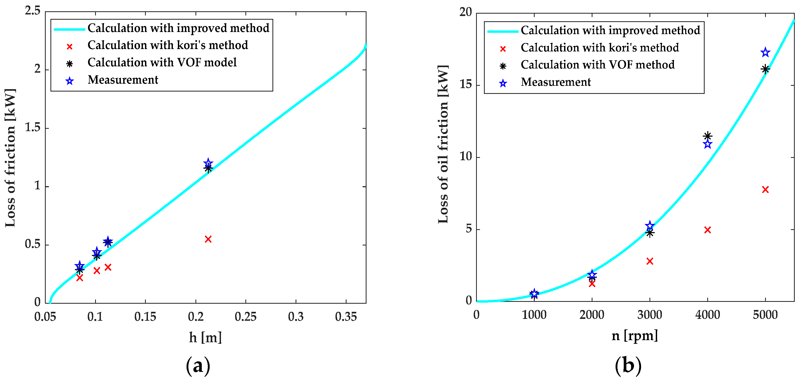
• The improved method analytical has higher computational accuracy than those previously studied. It is suitable for the early design of an oil-immersed cooling motor. When the design parameters need to be adjusted, the designer can quickly calculate the oil friction loss.
• The VOF model can accurately reflect the law of oil friction loss under the rotation speed and oil-soaked depth. The maximum error between theoretical calculation and testing data is less than 10%. It is useful in the later optimization design of the oil-immersed cooling motor, and the oil friction loss caused by the variation of local structure can be calculated by the model.
• The oil friction loss is proportional to the first power of the oil-soaked depth and the 2nd–3rd power of the rotational speed.

References

1. Wang, X.; Gao, P. Application of Equivalent Thermal Network Method and Finite Element Method in Temperature Calculation of in-Wheel Motor. Electr. Mach. Control 2016, 31, 26–33. [Google Scholar]
2. Guo, F.; Zhang, C. Oil-Cooling Method of the Permanent Magnet Synchronous Motor for Electric Vehicle. Energies 2019, 12, 2984. [Google Scholar] [CrossRef] [Green Version]
3. Liu, C.; Gerada, D.; Xu, Z.; Chong, Y.C.; Michon, M.; Goss, J.; Zhang, H. Estimation of Oil Spray Cooling Heat Transfer Coefficients on Hairpin Windings with Reduced-parameter Models. IEEE Trans. Transp. Electrif. 2020, 7, 793–803. [Google Scholar] [CrossRef]
4. Ponomarev, P.; Polikarpova, M.; Pyrhonen, J. Thermal modeling of directly-oil-cooled permanent magnet synchronous machine. In Proceedings of the XXth International Conference on Electrical Machines, Marseille, France, 2–5 September 2012; IEEE: Manhattan, NY, USA; pp. 1882–1887. [Google Scholar]
5. Zeng, J.; Sun, X.; Qian, Z. Thermal simulation of an oil-cooled permanent magnet synchronous motor. In Proceedings of the 2017 IEEE International Electric Machines and Drives Conference (IEMDC), Miami, FL, USA, 21–24 May 2017; pp. 1–7. [Google Scholar]
6. Ponomarev, P.; Polikarpova, M.; Pyrhonen, J. Conjugated fluid-solid heat transfer modeling of a directly-oil-cooled PMSM using CFD. In Proceedings of the International Symposium on Power Electronics Power Electronics, Electrical Drives, Automation and Motion, Sorrento, Italy, 20–22 June 2012; IEEE: Manhattan, NY, USA, 2012; pp. 141–145. [Google Scholar]
7. Kim, S.C.; Kim, W.; Kim, M.S. Cooling performance of 25 kW in-wheel motor for electric vehicles. Int. J. Automot. Technol. 2013, 14, 559–567. [Google Scholar] [CrossRef]
8. Zhang, Y.; Shen, Y.H.; Zhang, W.M. Multi-Objective Optimization Analysis of Motor Cooling System in Articulated Dump Truck. Adv. Mater. Res. 2012, 383–390, 4715–4720. [Google Scholar] [CrossRef]
9. Ye, L.; Tao, F.; Qi, L.; Xuhui, W. Experimental investigation on heat transfer of directly-oil-cooled permanent magnet motor. In Proceedings of the 2016 19th International Conference on Electrical Machines and Systems (ICEMS), Chiba, Japan, 13–16 November 2016; IEEE: Manhattan, NY, USA, 2017; pp. 1–4. [Google Scholar]
10. Davin, T.; Pellé, J.; Harmand, S.; Yu, R. Experimental study of oil cooling systems for electric motors. Appl. Therm. Eng. 2015, 75, 1–13. [Google Scholar] [CrossRef]
11. Sugimoto, S.; Kori, D. Cooling Performance and Loss Evaluation for Water- and Oil-Cooled without Pump for Oil. In Proceedings of the 2018 XIII International Conference on Electrical Machines (ICEM), Alexandroupoli, Greece, 3–6 September 2018; pp. 1136–1141. [Google Scholar]
12. Montonen, J.; Nerg, J.; Polikarpova, M.; Pyrhönen, J. Integration Principles and Thermal Analysis of an Oil-Cooled and -Lubricated Permanent Magnet Motor Planetary Gearbox Drive System. IEEE Access 2019, 7, 69108–69118. [Google Scholar] [CrossRef]
13. Nutakor, C.; Montonen, J.; Nerg, J.; Heikkinen, J.; Sopanen, J.; Pyrhönen, J. Development and validation of an integrated planetary gear set permanent magnet electric motor power loss model. Tribol. Int. 2018, 124, 34–45. [Google Scholar] [CrossRef]
14. Ponomarev, P.; Polikarpova, M.; Heinikainen, O.; Pyrhönen, J. Design of integrated electro-hydraulic power unit for hybrid mobile working machines. In Proceedings of the 2011 14th European Conference on Power Electronics and Applications, Birmingham, UK, 30 August–1 September 2011; IEEE: Manhattan, NY, USA, 2011. [Google Scholar]
15. Hirt, C.W.; Nichols, B.D. Volume of fluid (VOF) method for the dynamics of free boundaries. J. Comput. Phys. 1981, 39, 201–225. [Google Scholar] [CrossRef]
16. Park, M.H.; Kim, S.C. Thermal characteristics and effects of oil spray cooling on in-wheel motors in electric vehicles. Appl. Therm. Eng. 2019, 152, 582–593. [Google Scholar] [CrossRef]
17. Liu, M.; Li, Y.; Ding, H.; Sarlioglu, B. Study on ATF Oil Resistant Insulating Material and System for Electric Vehicle Motors. Insul. Mater. 2018, 2, 18–22. [Google Scholar]
Figure 1. Abridged general view.
Wevj 12 00164 g001
Figure 2. 3D structure.
Wevj 12 00164 g002
Figure 3. Fluid domain.
Wevj 12 00164 g003
Figure 4. VOF numerical model.
Wevj 12 00164 g004
Figure 5. The testing platform.
Wevj 12 00164 g005
Figure 6. The oil distribution at oil-soaked depth h = 0.1125 m: (a) the oil distribution when the rotor is still; (b) the oil distribution when the rotation speed is at n = 1000 rpm.
Wevj 12 00164 g006
Figure 7. The velocity field of oil at rotation speed n = 1000 rpm.
Wevj 12 00164 g007
Figure 8. The convergence curve of the loss.
Wevj 12 00164 g008
Figure 9. Comparison between the calculation with three methods and testing values of the oil friction loss: (a) relationship between oil friction loss and the oil-soaked depth h; (b) relationship between oil friction loss and the rotation speed n.
Wevj 12 00164 g009