1. Introduction
In order to limit carbon emissions and its consequences, the European Union (EU) has set ambitious greenhouse gas reduction targets. Greenhouse gas emissions are to be reduced by 40% by 2030 and by at least 80% by 2050 compared to 1990. The transportation sector has a major impact on the achievement of these goals since it accounts for 19.8% of EU greenhouse gas emissions [
1]. The transportation sector is the only sector with increased greenhouse gas emissions since 1990, and also the only sector for which the EU does not expect a reduction of 80% by 2050 [
2].
Electrically powered vehicles seem to be the ideal solution to this problem. For this, however, the electric powertrain must be designed as realistically and precisely as possible to represent the actual driving behavior of the driver in order to prevent unnecessary over dimensioning and the associated increase in energy consumption and battery aging, which in turn leads to a reduced driving range [
3]. In order to describe this driving behavior, vehicle developers need precise knowledge of the real vehicle use case, the driving speed, acceleration, stop phases, and the covered distance.
By recording and evaluating real driving data in fleet tests, the described parameters could be determined. One way of displaying these parameters is by using driving cycles. These speed-time profiles play an important role in the development process of vehicles in order to simulate the behavior of a vehicle, and thus, enable an insight into the behavior during the real operation [
4]. Standardized driving cycles could provide an initial assessment but generally, only reflect everyday driving to a limited extent and are, therefore, not significant enough for a realistic determination [
5].
The most significant method to determine reliable, realistic driving behavior lies in the evaluation of real driving data. Therefore, real driving data were collected and analyzed within the scope of this paper. The driving data could then be used to create a representative driving cycle for different drivers and vehicle classes in order to investigate different driving behaviors. Using the operating points of the created driving cycles, the necessary machine design could be derived and the different required machine characteristics can be identified.
2. State of the Art
State of the art first introduces the classification of different vehicle classes, since they exhibit different mobility behaviors, e.g., city and motorway journeys have different requirements regarding the powertrain [
6]. After an assessment of the regarded driving data, the resulting driving cycle can be derived depending on the significant driving behaviors and the impact on a realistic design of future electric powertrains can be analyzed.
2.1. Classification of Vehicle Categories
Vehicle classes are defined internationally in the International Organization for Standardization (ISO) 3833:1977. This standard distinguishes vehicle classes according to technical characteristics and is valid for all vehicles approved for road use. In the context of this work, a classification of the Kraftfahrtbundesamt (KBA) is used, which is used for the creation of the “Mobility in Germany” database (MiD) [
6]. The KBA distinguishes between four main vehicle classes—small cars, compact class, middle class, and large cars. The annual mileage of the different vehicle classes, are shown in
Table 1.
In addition to the classification of vehicles according to their technical characteristics, a classification according to the intended use of the vehicle could also take place using the MiD. The average distance traveled in a single journey considering their various purposes is shown in
Table 2.
This shows that on average, business trips require the most distance for a single trip, followed by leisure trips and home commute. The distance traveled for errands and to educational institutions shows the lowest average distance per journey.
2.2. Conventional Driving Cycles
Each vehicle class has different and typical mobility behavior. However, this is not only vehicle-specific, but also depends on the routes traveled. The MiD distinguishes between city, overland, and motorway journeys [
6]. For a more detailed differentiation, the roads could be divided according to the degree of street quality, the purpose of use, location in the city, and speed limit.
A driving cycle describes a fixed timetable for vehicle operation that allows an emissions test to be carried out under standardized laboratory conditions for high reproducibility. They are usually defined by vehicle speed and gear selection as a function of time. Emission levels depend on many parameters, including vehicle-related factors such as vehicle type and fuel type, as well as operational factors such as speed, acceleration, and gear selection. Therefore, different driving cycles have been developed for different mobility behaviors [
7].
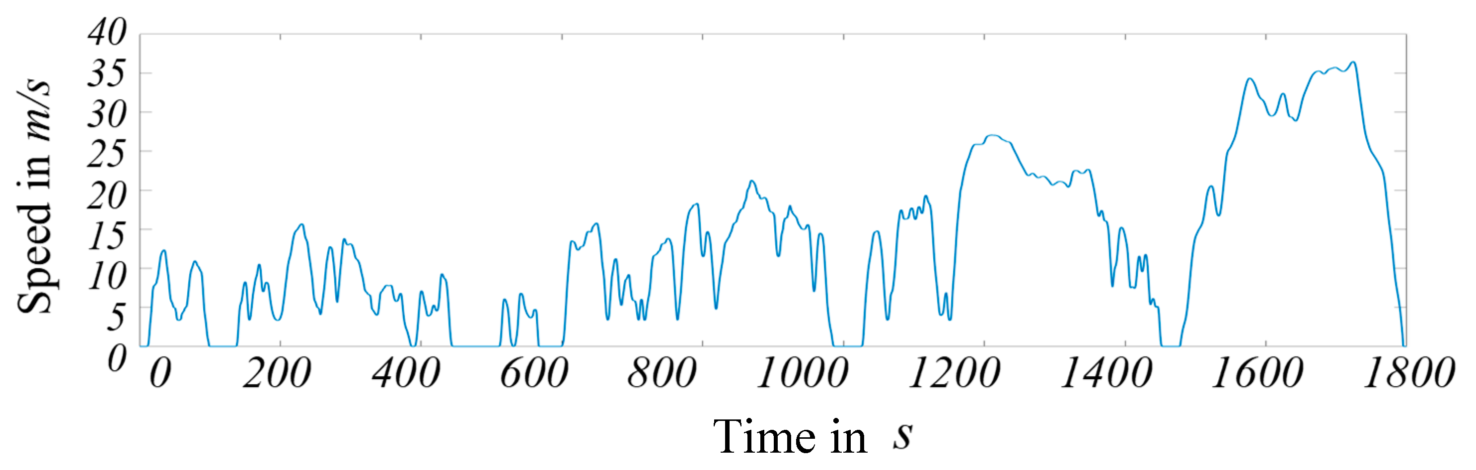
Driving cycles such as the New European Driving Cycle (NEDC) or the worldwide harmonized light vehicles test procedure (WLTP) are widely used to determine the consumption and emissions of vehicles. They are currently the subject of criticism, as they usually cannot reflect real consumption with satisfactory accuracy. Nevertheless, they can be used to generate comparable measurement results between different vehicles. The WLTP (
Figure 1) has been designed to be more dynamic with a significantly higher average and maximum accelerations. In addition to a longer driving time than the NEDC, the average and maximum speed were increased. With a cycle length of 23.25 km, it is also significantly longer than the NEDC [
8,
9,
10].
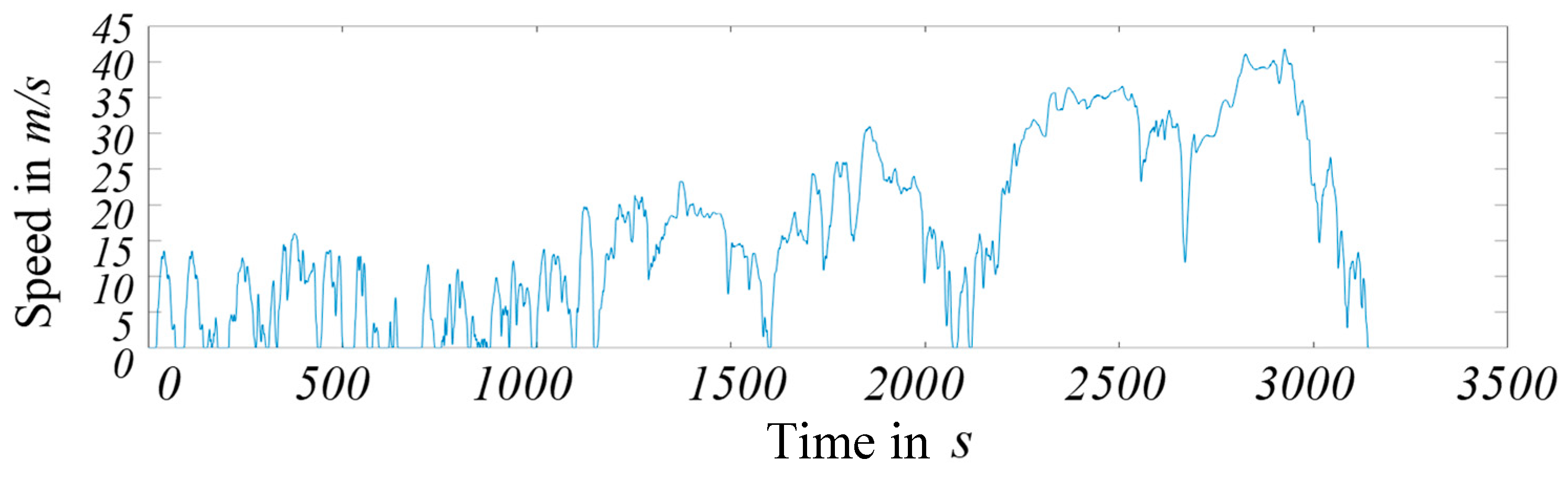
Another common conventional driving cycle is the Assessment and Reliability of Transport Emission Models and Inventory Systems (ARTEMIS) cycle. This cycle was generated using real, European driving data and has the goal of enabling the most realistic possible estimation of emissions for a variety of vehicles. It is divided into three segments-city, rural, and motorway (
Figure 2). The maximum speed of city driving is defined as 57.3 km/h, while the maximum speed of rural areas is set to 111.1 km/h [
11].
The city cycle, for example, essentially consists of portions of flowing, dense and congested traffic. This can be clearly seen in the number of stops, the duration of idle times, and the speeds driven. The driving cycles for rural traffic and motorway journeys are differentiated according to similar principles.
2.3. Methods for Creating a Driving Cycle from Real Data
There are various ways to create a driving cycle, whereas the most common methods use microtrips, acceleration speed matrices (AV matrix), or clusters. Since the raw data is often available in driving sections from a few minutes to several hours, it cannot be used directly for the creation of a driving cycle. First, these speed/time combinations must be divided into short sequences, so-called microtrips. A microtrip is defined as a speed-time curve between two consecutive stops [
12]. This method, in which the start and endpoints have a velocity of zero, is widely used in practice. However, if this method is to be used to divide motorway journeys into microtrips, it may happen that their duration does not lie within the range of the specified cycle length. SHI et al. [
12] define an optimal microtrip to have a maximum duration of 300 s in which the acceleration at the beginning and end is zero. This makes it possible to subdivide longer trips and take them into account when creating a cycle.
An AV matrix is a widely used method for categorizing driving behavior, where the acceleration and speed values of a driving sequence are linked by frequency. The speed and acceleration axis is divided into equal intervals so that each individual point of a driving situation can be clearly assigned in the matrix [
12,
13].
Cluster-analytical methods are used to combine data sets into homogeneous groups, called clusters [
14]. All clusters have a cluster center called centroid [
14]. The Kmeans cluster method is a partitioning method in which the dataset is first divided into a certain number of clusters. Each data point is then assigned to the center closest to it. After this assignment, the centers are recalculated using the current clusters, and the data points are reassigned to the closest centroids. This algorithm is repeated until the centers are hardly or no longer distinguishable [
15]. In this paper, microtrips are divided into a fixed number of groups by using Kmeans clustering.
3. Real Driving Data
The driving data analyzed in this paper were recorded by the Institute of Automotive Technology at the Technical University of Munich [
16]. The data originate from different test series in the private, business, and taxi sector and was, therefore, collected using different vehicles. All necessary signals were recorded using sensors of smartphones with which each vehicle was equipped, using a recording rate of 1 Hz, as stated in [
17]. The x-, y- and z- coordinates, height differences, and speed profiles provide the main measuring points over time.
The recorded data are made up of 4034 datasets for private vehicles and 162,540 datasets for taxis. The private driving data were obtained by the research project sun2car within the e-GAP model municipality of Garmisch-Partenkirchen and focused on the investigation of customer acceptance behavior [
18]. The data sets were recorded by 58 private users, mostly driving an Audi A1 e-tron or A3 g-tron. The taxi data was recorded by 90 taxi drivers within the project Vem Taxi in the general area of Munich, including vehicles like the Mitsubishi i-MIEV, Mercedes e-Vito and the Tesla Model S, as well as a few medium-sized combustion engine vehicles. In total, an overall distance of 4,347,194 km and 145,869 driving hours were recorded [
17].
The maximum speed and requested torque, which depend on the required acceleration and required gradient behavior, are essential for the creation of a load spectrum for the powertrain. The acceleration
a is determined by the differentiation of the current and subsequent speed values
v divided by the time difference Δ
t.
To determine the gradient, it is relevant to calculate the difference in height that has been covered (Δ
elevn):
In addition to the difference in altitude, the distance traveled is required to determine the gradient, by calculating the quotient of the height difference and the horizontally traveled distance:
4. Analysis of Real Driving Data
With the assignment of gradient and acceleration, the relevant parameters are now assigned to the velocity. The classification into city, rural, and motorway was made on the basis of the ARTEMIS cycle [
8], as shown in
Table 3:
4.1. Speed Profile Taxi
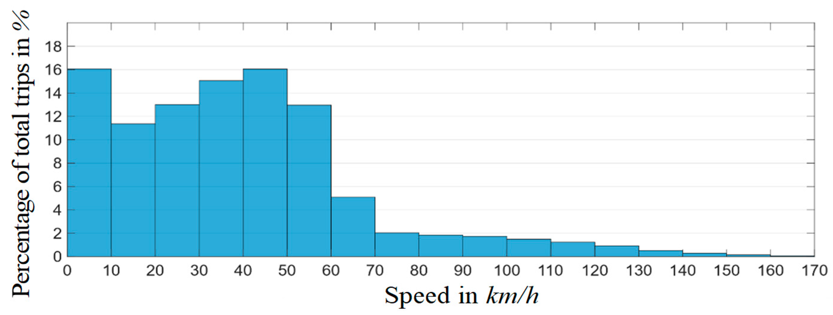
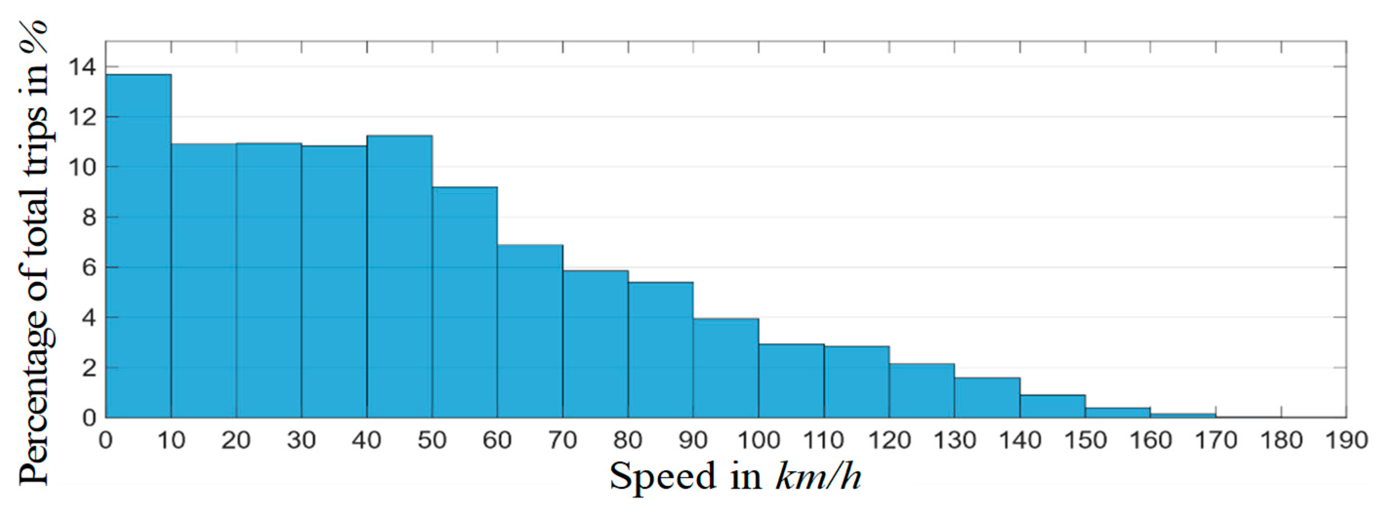
The speed profiles traveled by the recorded taxi trips could be classified into the main route types as follows: 82% city, 15% rural, and 3% motorway. Most of the taxi trips take place within the city. At 15% and 3%, respectively, the proportion of rural roads is comparatively small, while the proportion of motorways is particularly small. These values indicate that the main use of taxis is in the city or urban areas. The speed distribution of the recorded taxi trips is shown in
Figure 3.
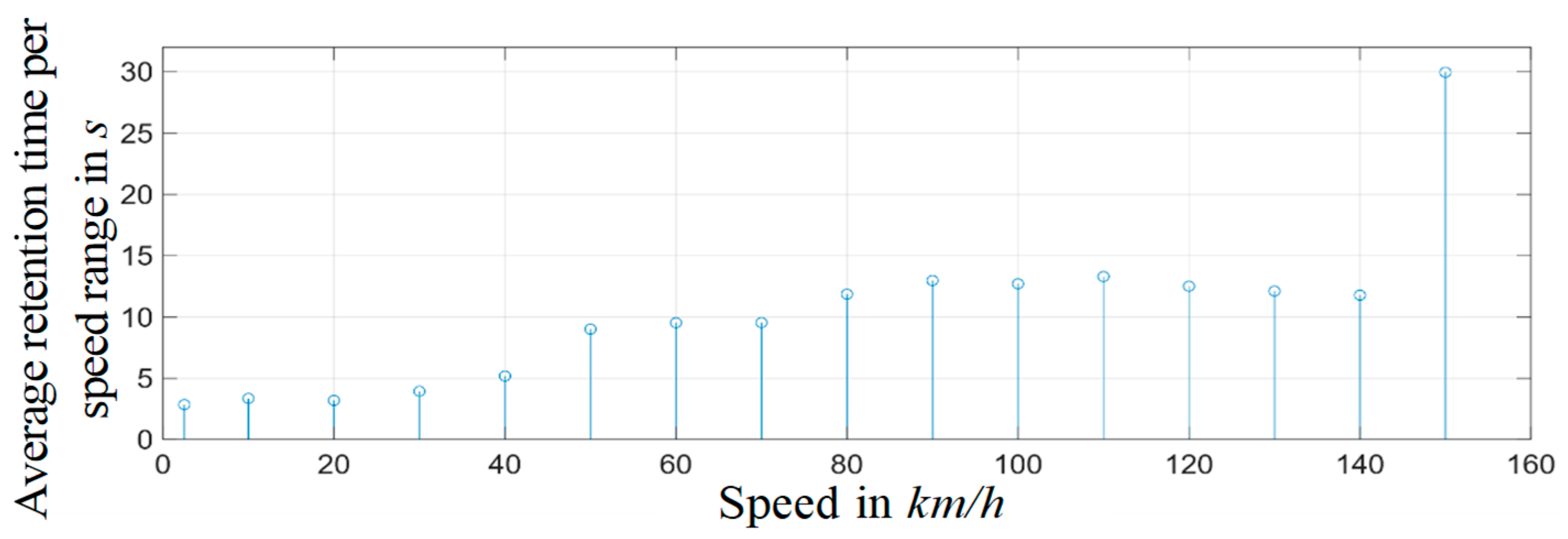
The majority of taxi journeys take place at speeds below 60 km/h, as could already be expected since 82% of the journeys are recorded in the city. From 70 km/h onwards, the frequency decreases steadily. The comparatively low frequency of trips in the range of 10 to 20 km/h is also noticeable. From this range, the frequency rises again up to 50 km/h. It could, therefore, be assumed that this is the desired speed of the drivers, in this case, the maximum possible speed in the city, but in some cases, lower speeds have to be driven due to traffic and road conditions. A further look at the retention times in each speed range serves to examine the speed profiles more closely (
Figure 4).
The retention times in the speed range below 50 km/h are comparatively short, i.e., they are rather “passed through” than held. This is due to the fact that the acceleration in this area is very high and the respective drivers attempt to reach the desired maximum allowed velocity quickly, e.g., after a traffic light or congested traffic. Above 150 km/h, the speed ranges are combined.
4.2. Speed Profile Private Vehicles
The speed analysis of private and commercial users also enables an initial, rough division into the three route types, with the resulting percentage as follows: 65% city, 27% rural, and 8% motorway. More than half of the measuring points are assigned to city trips, mainly in the Munich city area. Nevertheless, compared to the taxi trips, the share of rural road journeys has doubled, and the number of motorway journeys has almost tripled in direct comparison. It can be seen that private and commercial vehicles are driven outside the city more often than taxis. The speed distribution, resulting from the sample of private drivers, is shown in
Figure 5.
The range between 0 to 10 km/h is also the most frequently operated by private individuals and businesses. At speeds above 50 km/h, the frequency decreases, but not as steeply as for taxi drives, with an approximately linear decrease up to 170 km/h.
4.3. Acceleration Profile Taxi
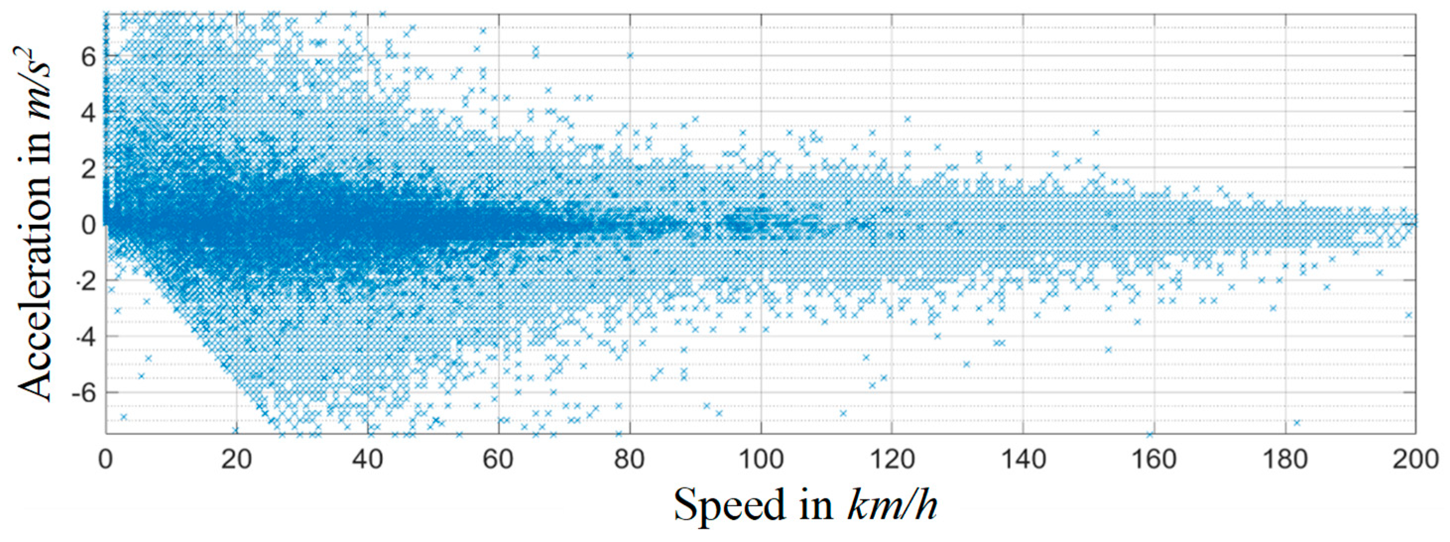
In order to enable an initial analysis and assessment of the driving data, the acceleration/speed combination can be regarded. The evaluated taxi data shows the following acceleration behavior in
Figure 6.
It can be seen that a rather small part of the accelerations are in high or low areas (light area), while a large part of the accelerations is close to the x-axis at low speeds (dark area). This shows that the maximum possible accelerations are rarely reached. Possible explanations for this are more comfortable driving behavior, as well as dense and congested traffic. For speeds over 30 km/h, the accelerations are approximately symmetrical to the x-axis. At lower speeds and negative accelerations, the data points form a linear trend. The explanation for this is that at low speeds, for reasons of comfort, the driver no longer brakes fully.
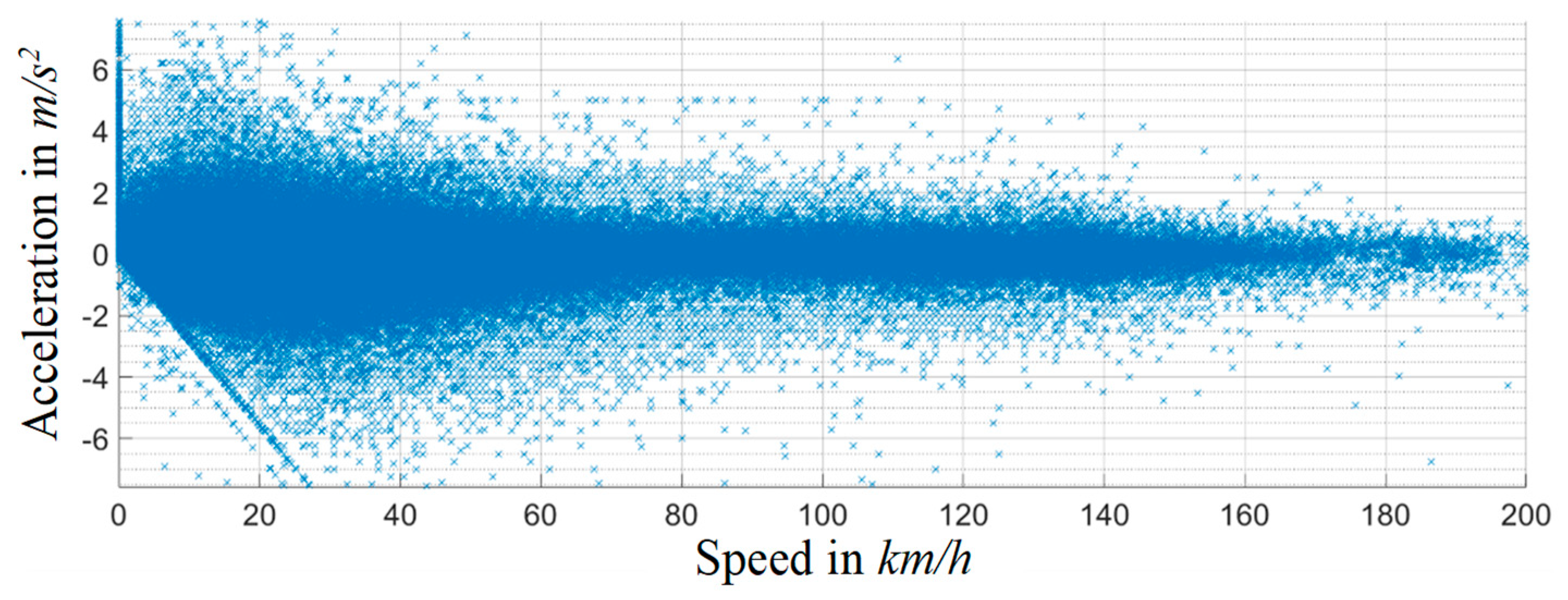
4.4. Acceleration Profile Private Vehicles
Figure 7 shows all acceleration-speed combinations for the recorded driving data of private drivers. The measured values are distributed similarly to the taxi data. With increasing speed, the acceleration decreases, but less steeply than for the taxi data. Also, the gap of the negative accelerations at low speeds is acutely more recognizable. The brighter, less frequented area is smaller than for taxi drivers. This is due to the higher speed levels for private trips, which increases the density of measuring points at higher speeds. Since the scattering of the acceleration points is smaller for private vehicles, it can also be assumed that the ownership of private vehicles leads to less aggressive acceleration behavior.
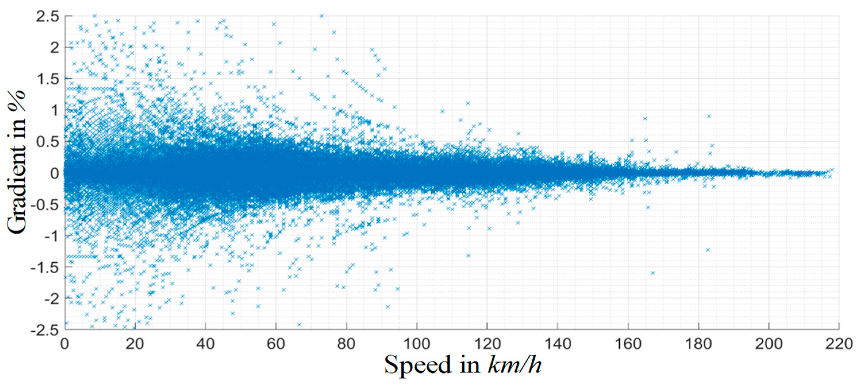
4.5. Gradient Distribution Taxi
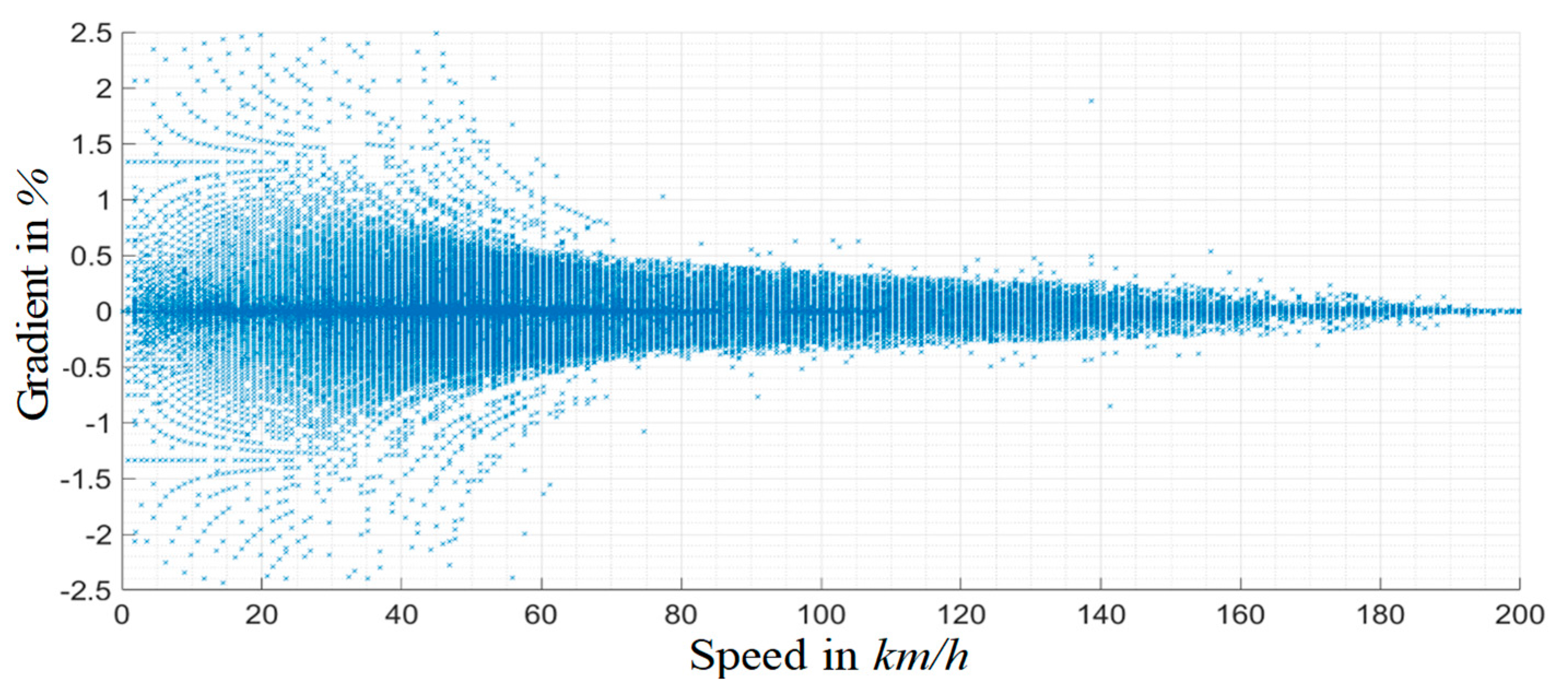
With regard to the design of the powertrain, the assignment of the gradient to the speed is also relevant.
Figure 8 shows the assignment of the gradient over the respective speed.
Over 64% of trips take place on a gradient of ∓0.5%, due to the circumstances in the Munich city area, where most of the data was recorded. The remaining gradients are distributed almost symmetrically around the x-axis. Thus, 7% of the journeys are still in the gradient area of ∓0.5–1.5%, as well as 3% in the gradient area of ∓1.5–2.5%. The remaining data points are distributed among the larger gradient areas. As the speed increases, the gradients decrease and vice versa.
4.6. Gradient Distribution Private Vehicles
The distribution of all gradients from the private driving data is shown in
Figure 9.
It can be seen that the gradients are also distributed approximately symmetrically around the x-axis. The main area of the gradients, i.e., from −0.5% to +0.5% is, however, approached less frequently than for the taxi data. From a gradient of ∓5%, the relative frequency for larger gradients is less than 1%. The gradients decrease with increasing speed, but more gradually than the taxi data. Up to 100 km/h, there are still noticeable deviations from the x-axis for the measured values. At maximum speed, only marginal gradients can be observed.
5. Results and Discussion
5.1. Creation of the Driving Cycle
The analysis uses the default parameters in
Table 4 based on existing driving cycles and investigations in [
8] in order to form the respective microtrips.
The reason for using thresholds is the diversity of the data collection. This reduces the probability that information about vehicle stops will be lost due to smoothing of the speed curve. The speed and acceleration thresholds determine when the vehicle is considered stationary or unaccelerated. The time threshold for parking was introduced for the case that the vehicle is permanently stationary. The vehicle is assumed to be parked if the speed does not exceed the speed threshold for the specified period. A consideration of stops at traffic lights or in traffic jams is, thus, taken into account, whereas parking the vehicle does not falsify the driving behavior due to long stops [
3].
A spectrum of 20 to 30 min is ideal to obtain a representative amount of driving characteristics [
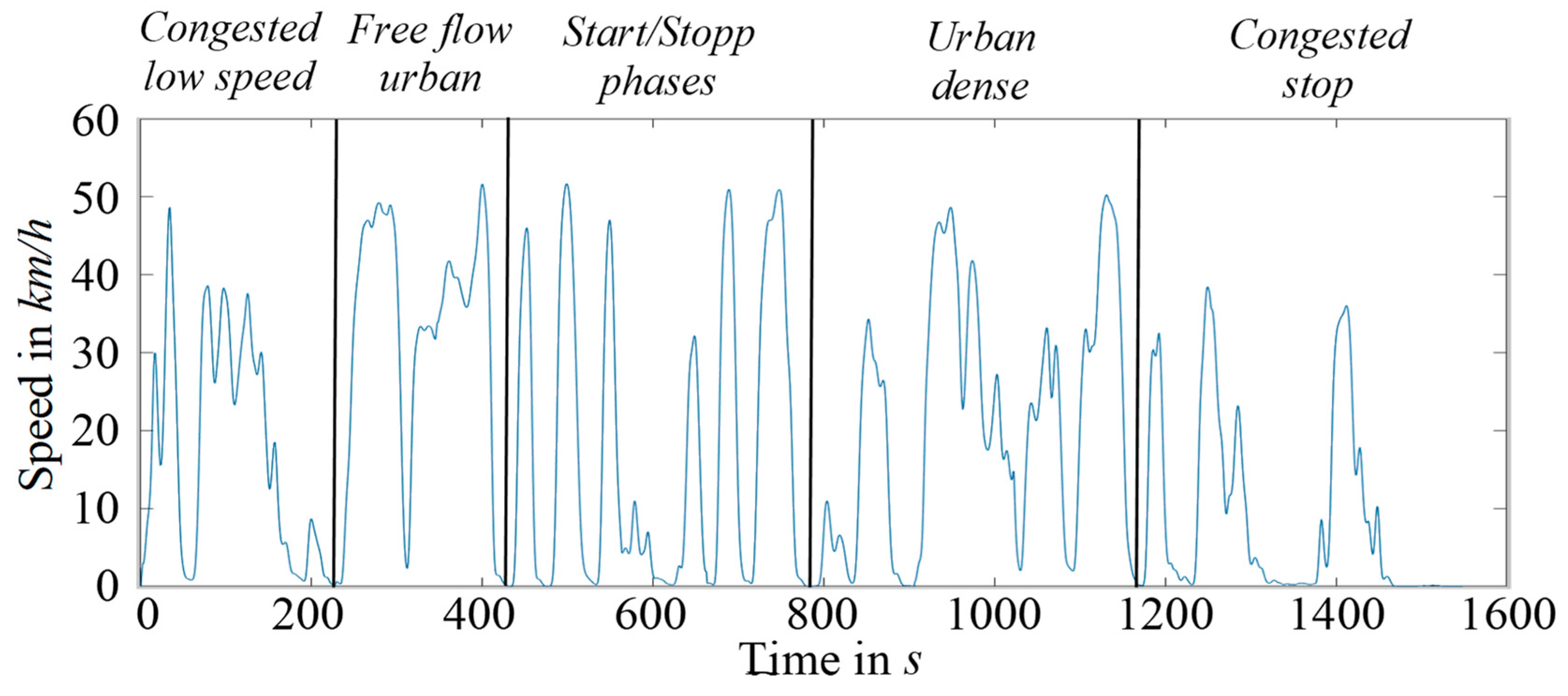
8]. However, the exact length of a driving cycle cannot be set to a fixed length, since it depends on the length of the respective characteristic microtrips used in the creation of the cycle, which could vary in length depending on the regarded driving data. In order to show exemplary results, the derived driving cycle based on the recorded real driving data for the taxi drivers is illustrated in
Figure 10.
It can be seen that in regard to the classification of the ARTEMIS and the KBA, the created driving cycle mostly demonstrates characteristics of an urban or city cycle. Considering the classification used in [
13], the derived driving cycle was divided into the illustrated sections. The first section from the beginning of the cycle to approximately 220 s into the cycle can be characterized as congested low-speed traffic. The following section to approximately 420 s symbolizes a version of free flow urban traffic. This section is followed by a long section with frequent Start/Stop phases, indicating a high number of consecutive traffic lights. From approx. 800 s to 1200 s; the traffic could be characterized as urban dense, followed by the last section of the cycle which represents a traffic behavior with frequent congestions and stops.
5.2. Requirements for Electric Machine Design
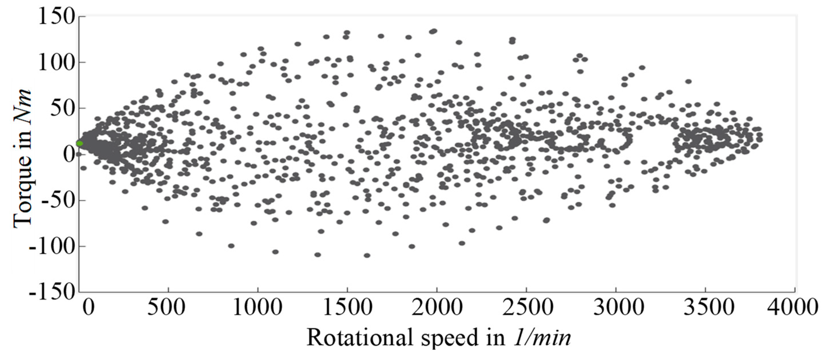
The operating points of a vehicle are individually dependent on the respective application and use case, have a direct impact on the overall machine and powertrain design and should, therefore, be considered in the future design process of electric vehicles. In the following
Figure 11, the operating points of the created driving cycle for the taxi driving data are illustrated, which are determined using the machine design tool presented in [
19] and a longitudinal dynamics simulation tool based on [
20].
The characteristics of a driving cycle are of great importance for the design of the powertrain of a vehicle, especially for the machine design. Therefore, the electric machine needs to be designed according to the occurring operating points of a specific vehicle and application. The operating points are dependent on the distribution of torque to rotational speed combinations during vehicle operation. They determine the necessary maximum torque, maximum rotational speed, and nominal values of the electric machine. The maximum vehicle speed is determined by the necessary maximum rotational speed of the electric machine, which mainly depends on the machine topology and incurred centrifugal forces. The continuous power, defined by the cooling type and dimensions of the machine, is determined by the frequency that the maximum torque is operated within a certain period of time, e.g., how many times in a row a red traffic light is dynamically approached or the number of accelerations on a winding mountain path, i.e., maximum cruise speed and acceleration time from 0–100 km/h. The maximum torque determines the diameter of the electric machine and depends on the maximum current of the implemented power electronics. It characterizes the overload capability of an electric machine and poses a great advantage for dynamic acceleration [
21].
Overall, the operating points of the created cycle based on real driving data from taxi trips show a combination of high torque and relatively low rotational speed. The distribution shows an elliptical form, with frequent operating points located in low rotational speed and low-torque areas and higher rotational speeds with low torque combinations, as well as high torque areas in between. This is primarily due to the fact that most of the driving data was recorded in the city and high rotational speeds are not obtained due to lack of frequent motorway trips. The high torque supports the assumption of a high frequency of start/stop phases, e.g., consecutive traffic lights, as well as congested traffic.
For the machine design, this means that the focus should be on operating points with high torque and low rotational speed combinations. The low rotational speed indicates low mechanical losses, e.g., bearings and air-friction in the machine design. Due to the high torque, howevers great emphasis needs to be set on the copper losses of the machine, since higher torque directly correlates to the current flow of the machine. Therefore, the machine needs to be designed for higher current flow and nominal power, as well as the consideration of higher insulation. This leads to a general increase in the diameter of the overall machine, which needs to be considered in the package design.
5.3. Cycle Efficiency
In order to showcase exemplary results in this paper, an analysis of the electric machine of the BMW i3 was conducted using conventional, as well as the created driving cycle. The BMW i3 offers a reasonable comparison since most machine parameters are released by the Original Equipment Manufacturer (OEM). An overview of the vehicle parameters is presented in
Table 5; the respective literature is indicated behind each value. The values for the auxiliary consumers [
22] and gear efficiency are a rough estimation since the aim is solely a relative comparison.
The electric machine design of the regarded BMW i3 model is specified in
Table 6. The electric machine of the BMW i3 is a hybrid permanent magnet synchronous machine (Hybrid PSM) combined with a reluctance machine with double-layered integrated permanent magnets, liquid cooling, and an overall weight of about 55 kg [
25]. Several input parameters for the 2016 model were defined prior to the analysis in this paper using [
25,
26,
27] and the technical data sheet of the BMW Group [
23].
The input parameters of the electric machine can then be used to calculate the efficiency diagram using the open-source electric machine design tool presented in [
19]. In order to calculate the energy consumption and range of the exemplary vehicle with the conventional and created driving cycles, a longitudinal dynamics simulation (LDS) using a backward simulation based on [
19] with a time step of 1 s is initiated, considering the driving cycles, vehicle parameters, as well as the results from the electric machine design. The LDS tool implemented by the institute of the authors is used to calculate the energy consumption, range in the cycle, as well as cycle efficiency for the respective machine design and regarded driving cycles, see
Table 7. The respective cycle efficiency is calculated using the efficiency diagrams of the machine in combination with the speed/torque combinations of the operating points of the vehicle in each driving cycle.
The results of the conducted LDS show, that for the same electric machine the cycle efficiency during operation deviates due to different operating points. Therefore, solely increasing the overall machine efficiency is not reasonable without considering the actual operating points of the desired application use case.
6. Summary
Driving cycles, in general, represent an important tool in order to enable a representative comparison between different vehicles. But they reach their limitation in regard to the actual driving characteristics of different use cases when trying to illustrate a variety of vehicle classes and driving behaviors realistically.
It was shown that different applications, in this case, taxis and private drivers, have different mobility behaviors. The mobility profiles of taxi drivers and private or commercial drivers differ, especially in the speed distribution. In the case of taxi journeys, the city area is more pronounced with speeds below 60 km/h, while for private drivers, more journeys take place at higher speeds. For the acceleration behavior, only small differences between the taxi and the private or commercial users can be seen. The gradients were somewhat lower for taxi journeys, which in turn can be attributed to the frequent inner-city journeys.
Driving cycles, however, differentiate primarily according to technical aspects and disregard the actual use case, e.g., even the maximum speed of the WLTP of approx. 130 km/h is not sufficient for driving on German motorways. For the private drivers analyzed in the regarded data sets, this affects more than 5% of all journeys. The maximum accelerations in the WLTP are considerably lower than those of the real data and are more in the range of the average values of the recorded driving data. The maximum speeds are higher for all investigated user groups than for the conventional driving cycles. The average speed of the driving data is higher than in the driving cycles, at least for the private drivers. The actually requested maximum accelerations of both user groups are far higher than the maximum accelerations of the conventional driving cycles. Since driving cycles are not recorded with gradients, no comparison between real data and driving cycles could be made for this parameter.
In conclusion, the utilization of driving cycles is reasonable to a certain extent when solely a relative comparison of the energy consumption of different vehicles is desired, but they reach their limitation when trying to represent the actual energy consumption during realistic operation. Furthermore, applying one or a few driving cycles to a variety of different application use cases is not realistic, since the requirements and efficiency during operation of not only the electric machine but the overall vehicle strongly depend on the actual use case and operating points individually. For electric vehicles, for example, the full torque is available from the first revolution and can thus achieve significantly higher maximum accelerations. Therefore, a driving cycle for electric vehicles should have a higher maximum acceleration than a cycle for combustion engines. This makes it possible to achieve a more dynamic driving behavior and must be taken into account in the design process. Therefore, higher requirements should be integrated into driving cycles and the application (e.g., taxi, commercial, private use), the vehicle classification (e.g., small or large vehicles such as sport utility vehicle (SUV), trucks, and city vehicles), as well as nowadays the type of powertrain (e.g., combustion, electric) need to be considered in the design process of driving cycles in the future.
Author Contributions
As the first author, S.K. drew up the overall concept of this paper, contributed the tool for the application-based design of the electric machines and conducted the requirement analysis. L.B. supported during his semester thesis with the creation of the data analysis. M.L. made an essential contribution to the conception of the research project. He revised the paper critically for important intellectual content. M.L. gave final approval of the version to be published and agrees to all aspects of the work. As a guarantor, he accepts responsibility for the overall integrity of the paper.
Funding
This work was funded by the organization Bayern Innovativ within the research project DeTailED—Design of Tailored Electrical Drivetrains.
Conflicts of Interest
The authors declare no conflict of interest. The funders had no role in the design of the study; in the collection, analyses, or interpretation of data; in the writing of the manuscript, or in the decision to publish the results.
References
- European Commission. Factsheet Climate Change 2015; European Commission: Brüssel, Belgium, 2015. [Google Scholar]
- European Commission. The Roadmap for Transforming the EU into a Competitive, Low-Carbon Economy by 2050; European Commission: Brüssel, Belgium, 2011. [Google Scholar]
- Proff, H.; Fojcik, T.M. Mobilität und Digitale Transformation: Technische und Betriebswirtschaftliche Aspekte; Gabler: Wiesbaden, Germany, 2018. [Google Scholar]
- Robert, F. Fahrzyklen. Available online: https://tu-dresden.de/bu/verkehr/iad/fm/forschung/forschungsfelder/ebr/fahrzyklen?set_language=en (accessed on 24 September 2019).
- Bargende, M.; Reuss, H.-C.; Wiedemann, J. 18. Internationales Stuttgarter Symposium: Automobil-und Motorentechnik; Springer Vieweg: Wiesbaden, Germany, 2015. [Google Scholar]
- Bundesministerium für Verkehr und digitale Infrastruktur. Available online: http://www.mobilitaet-in-deutschland.de/pdf/MiD2017_Ergebnisbericht.pdf (accessed on 24 September 2019).
- Barlow, T.J.; Latham, S.; McCrae, I.S.; Boulter, P.G. A Reference Book of Driving Cycles for Use in the Measurement of Road Vehicle Emissions; TRL: Berkshire, UK, 2009. [Google Scholar]
- Giakumes, E.G. Driving and Engine Cycles; Springer Nature: Cham, Switzerland, 2017. [Google Scholar]
- Verband der Automobilindustrie, E.V. WLTP—Neues Testverfahren Weltweit am Start: Fragen und Antworten zur Umstellung von NEFZ auf WLTP; VDA: Berlin, Germany, 2018. [Google Scholar]
- Verband der Automobilindustrie. WLTP—Weltweit Harmonisierter Zyklus für Leichte Fahrzeuge. Available online: https://www.vda.de/de/themen/umwelt-und-klima/ab-gasemissionen/wltp-weltweit-harmoni sierter-zyklus-fuer-leichte-fahrzeuge.html (accessed on 24 September 2019).
- Dieselnet. Common Artemis Driving Cycles (CADC). Available online: https://www.dieselnet.com/standards/cycles/artemis.php (accessed on 24 September 2019).
- Shi, S.; Wei, S.; Kui, H.; Liu, L.; Huang, C.; Liu, M. Improvements of the design method of transient driving cycle for passenger car. In Proceeding of the 2009 IEEE Vehicle Power and Propulsion Conference, Dearborn, MI, USA, 7–10 September 2009. [Google Scholar]
- André, M.; Keller, M.; Sjödin, Å.; Gadrat, M.; Crae, I.M. The ARTEMIS European Tools for Estimating the Pollutant Emissions from Road Transport and their Application in Sweden and France. In Proceedings of the 17th International Conference Transport and Air Pollution, Graz, Austria, 19–20 June 2008. [Google Scholar]
- Stein, P.; Vollnhals, S. Grundlagen clusteranalytischer Verfahren; University Duisburg-Essen: Duisburg, Germany, 2011. [Google Scholar]
- Clusteranalyse: K-Means. Available online: http://www-m9.ma.tum.de/material/felix-klein/clustering/Methoden/K-Means.php (accessed on 24 September 2019).
- Wittmann, M.; Lohrer, J.; Betz, J.; Jäger, B.; Kugler, M.; Klöppel, M.; Waclaw, A.; Hann, M.; Lienkamp, M. A holistic framework for acquisition, processing and evaluation of vehicle fleet test data. In Proceedings of the 20th International Conference on Intelligent Transportation Systems, Yokohama, Japan, 16–19 October 2017. [Google Scholar]
- Jäger, B.; Hann, M.; Lienkamp, M. VEM-Virtuelle Elektromobilität im Taxi—und Gewerbeverkehr München: Neuartiger Ansatz zur Untersuchung von technischen, wirtschaftlichen und ökologischen Gesichtspunkten einer elektrifizierten Fahrzeugflotte; Technische Universität München: Garching, Germany, 2016. [Google Scholar]
- Kugler, M.; Osswald, S.; Frank, C.; Lienkamp, M. Mobility Tracking System for CO2 Footprint Determination. In Proceedings of the AutomotiveUI ′14 6th International Conference on Automotive User Interfaces and Interactive Vehicular Applications, Seattle, WA, USA, 17–19 September 2014. [Google Scholar]
- Kalt, S.; Erhard, J.; Danquah, B.; Lienkamp, M. Electric Machine Design Tool for Permanent Magnet Synchronous Machines. In Proceedings of the International Conference on Ecological Vehicles and Renewable Energies (EVER), Monte-Carlo, Monaco, 8–10 May 2019. [Google Scholar]
- Pischinger, S.; Seiffert, U. Vieweg Handbuch Kraftfahrzeugtechnik; Springer Vieweg: Wiesbaden, Germany, 2016. [Google Scholar]
- Juraschek, S.; Buchner, A.; Schinnerl, B. Die elektrische Antriebstechnologie der BMW Group. In Proceedings of the International Vienna Motor Symposium, Vienna, Austria, 26–27 April 2018. [Google Scholar]
- Wallentowitz, H.; Freialdenhoven, A.; Olschewski, I. Strategien zur Elektrifizierung des Antriebstranges—Technologien, Märkte und Implikationen; Springer Nature: Cham, Switzerland, 2010. [Google Scholar]
- BMW Group, Technische Daten BMW i3. Available online: https://www.press.bmwgroup.com/deut schland/article/attachment/T0259598DE/359586 (accessed on 24 September 2019).
- ADAC Autotest BMW i3. Available online: https://www.adac.de/_ext/itr/tests/Autotest/AT5542_ BMW_i3_94_Ah/BMW_i3_94_Ah.pdf (accessed on 24 September 2019).
- Staton, D.; Goss, J. Open Source Electric Motor Models for Commercial EV & Hybrid Traction Motors. In Proceedings of the CWIEME, Berlin, Germany, 20–22 June 2017. [Google Scholar]
- Elektroauto-News.net. Test- und Fahrbericht des BMW i3—eine Woche elektrifiziert unterwegs. Available online: https://www.elektroauto-news.net/bmw-i3-test-fahrbericht-erfahrung (accessed on 24 September 2019).
- Merwerth, J.; BMW Group. The Hybrid-Synchronous Machine of the New BMW i3 & i8. Available online: http://hybridfordonscentrum.se/wp-content/uploads/2014/05/20140404_BMW.pdf (accessed on 24 September 2019).
© 2019 by the authors. Licensee MDPI, Basel, Switzerland. This article is an open access article distributed under the terms and conditions of the Creative Commons Attribution (CC BY) license (http://creativecommons.org/licenses/by/4.0/).


