Abstract
The electrification of bus-based public transportation contributes to the goal of reducing the adverse environmental impacts caused by urban transportation. However, the penetration of electric vehicles has been slow due to their lower vehicle range and total costs in comparison to vehicles driven by internal combustion engines. By improving the powertrain efficiency, the total costs can be reduced for the same vehicle range. Therefore, this paper proposes a holistic design exploration approach to investigate and identify the optimal powertrain concept for electric city buses based on the component costs and energy consumption costs. The load profiles of speed, slope, and passenger occupancy profiles are derived for a selected bus route in Singapore, which is used in a powertrain design exploration for a 30-passenger vehicle. Six different powertrain architectures are analyzed, together with single and multi-speed gearbox configurations, to identify the optimal powertrain architecture and the resulting component sizes. The powertrain configurations are further analyzed in terms of their influence on the vehicle characteristics and total costs. Multi-motor configurations were found to have better vehicle characteristics and lower total costs in comparison to single rear motor configurations. Concepts with motors on the front and a rear axle could shift the load points to a higher efficiency region, resulting in lower energy consumption and energy costs. The optimal powertrain concept was a fixed-speed two-motor configuration, with a booster motor on the front axle and a motor on the rear axle.
1. Introduction
Electrification of the powertrain has been considered as one of the most viable solutions in the automotive industry for reducing the environmental impacts of urban mobility and hence improving the air quality. Governments are implementing strategies to electrify road-based public transportation systems. To evaluate the benefits of battery electric vehicles in comparison to alternative technologies like diesel, alternative fuel, hybrid electric, or fuel cell electric buses, research has focused on life cycle assessments regarding costs and carbon dioxide emissions [1,2,3]. Further investigations have addressed the design of the required charging infrastructure [4,5] and the respective impact on the battery capacity of the bus [6,7]. Although vehicle concept optimization and powertrain concept optimization represent a state of research for electric passenger cars and enable the identification of an optimal solution regarding multi-criteria design objectives [8,9,10,11], there is limited research at the vehicle concept level for electric city buses.
The powertrain concept is a subsystem of the vehicle concept, which significantly influences the energy consumption, and thus the range, of an electric vehicle. The powertrain consists of a battery, power electronics, an electric motor, and transmission. To improve the efficiency of the powertrain, research has been conducted at various levels, ranging from component improvements [12,13,14,15] and topology/structure [16,17] to vehicle concept level optimization [9]. Lajunen [18] investigated different powertrain configurations for electric city buses and showed differences in the energy consumptions of up to 11%, in comparison to a single rear motor configuration. However, the influence of component sizing was not investigated and only five powertrain configurations were compared. Krapf et al. [19] conducted a holistic design exploration to identify the optimal powertrain configuration for electric city buses. The results showed that the overall efficiency of the powertrain is strongly influenced by the load points arising from the driving resistances. The powertrain structure, transmission design, and motor sizing were thus varied to identify concepts where the load points were shifted to regions of a higher efficiency. However, a constant passenger load was used, which could have resulted in an imprecise estimation of the load points, leading to an improper design of the powertrain concept.
Therefore, this paper derives the load profiles for a selected bus route in Singapore by obtaining the speed, slope, and passenger occupancy profiles. The resulting load profiles are subsequently used in a holistic and broad powertrain design exploration for a 30-passenger electric city bus. The impacts of the respective design decisions on the energy consumption, as well as on the powertrain costs, of electric city buses are evaluated to identify an optimal powertrain configuration. The results are compared against load profiles with a constant average passenger occupancy to evaluate the influence of passenger mass variation on the powertrain design.
2. Methodology
The powertrain design for a 30-passenger electric bus that would drive on a specific route in Singapore is analyzed in this paper. Figure 1 shows the overall approach of this paper, consisting of input, calculation, and optimization stages. The inputs are the derived load profiles of speed, passenger occupancy and slope profiles for the route, the vehicle parameters, and the requirements that the powertrain design must satisfy. In the calculation step, a powertrain design is created using the vehicle parameters of the powertrain architecture, motor power, number of motors, and gears. The mass of the powertrain design is calculated, which, along with the vehicle parameters and load profiles, is used in a longitudinal dynamics simulation to calculate the energy and total costs. In the optimization step, the vehicle characteristics of top speed, range, acceleration, and gradeability are evaluated and the best concepts that fulfil the requirements are identified through the design exploration.
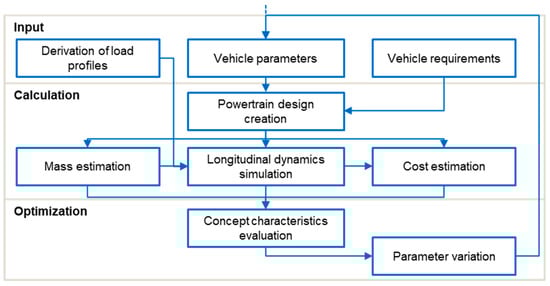
Figure 1.
Powertrain concept optimization methodology.
Angerer et al. [16] summarized existing powertrain concept optimization approaches and provided the basis for the choices of modeling methods. Based on [14], an optimization framework was implemented in MATLAB, as demonstrated in Figure 1, and a forward simulation approach was used to simulate the vehicle longitudinal dynamics in MATLAB Simulink.
The powertrain design can improve the energy consumption through three major effects:
- Powertrain weight;
- Powertrain efficiency;
- Load Point Shifting.
The framework enables the simulation of a variation of the component type, the component size, and the powertrain architecture, to investigate the influence on the powertrain weight and overall efficiency. Furthermore, multiple motor configurations and multi-speed transmissions can shift the load point and move the operation towards areas of a higher motor efficiency.
2.1. Derivation of a Realistic Speed and Slope Profile
A speed profile for the vehicle is required to calculate the operational load points of the powertrain and the resulting energy consumption. Koch et al. [20] provided the optimal speed profile of the vehicle for the selected bus route, assuming that the vehicle drives on a dedicated bus lane without traffic, since the vehicle under consideration would have similar operational characteristics. The problem was formulated as an optimal control problem using a dynamic programming algorithm, to obtain the optimal speed profile for the route, as shown in Figure 2. The derived speed profile is further used as an input for the longitudinal vehicle simulation to calculate the energy consumption and in the estimation of the passenger occupancy using the inter-stop travel time.
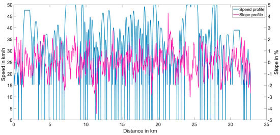
Figure 2.
Derived speed and slope profiles.
In addition, the road gradient influences the energy consumption of the vehicle. Therefore, the slope profile along the route was calculated by combining the bus route coordinates with satellite elevation data [21]. Figure 2 shows the slope profile of the route (in %).
2.2. Estimation of Passenger Occupancy
The passenger mass significantly contributes to the resistive forces of the vehicle that the powertrain must overcome to drive. If the powertrain concept is developed for maximum loading, oversizing of the components may occur, which could lead to a lower operational efficiency [12]. The influence of the passenger mass variation should therefore be taken into consideration during the design of the powertrain concept.
The passenger occupancy in the vehicle along the route is evaluated through a fleet simulation. The fleet simulation is conducted in three steps. An origin-destination matrix of the passengers is first estimated to evaluate the flow of passengers between stops, followed by calculation of the passenger arrival time at each bus stop and the simulation of vehicles departing and arriving at bus stops for a given timetable. The boarding and alighting process of passengers is subsequently simulated to obtain the passenger occupancy for each vehicle along the route.
The origin-destination (O-D) matrix is estimated by analyzing the hourly boarding and alighting passenger counts at each stop obtained from the smart card data of the public transport network. The origin and destination of the passenger flow along the route are reconstructed from the data using the Bayesian inference model proposed by Li [22]. Figure 3 shows the flow of passengers along the route and introduces the variables used in the inference model, where yi is the count of passengers boarding at stop i, zj is the count of passengers alighting at stop j, and xij is the number of passengers on-board the vehicle. The inference model uses a Markov chain to calculate the alighting probability matrix Pij, using the transitional probability qij, that a passenger will alight at stop i given that the passenger is in the vehicle at the i-1 stop, as shown in Equation (1). The probability qj is calculated in a Bayesian analysis by using a beta distribution to calculate the posterior probability, which is taken to be the posterior mean of the beta distribution, given by Equation (2). The alighting probability matrix is calculated by substituting the transitional probability into Equation (1) from which the trip O-D matrix is estimated using Equation (3).
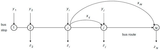
Figure 3.
Flow of passengers along the route [22].
To calculate the passenger occupancy in each operating vehicle, the passenger arrival and the vehicle fleet are simulated for the operational hours of the service. The arrival time of each passenger at each bus stop is calculated by modeling the passenger arrival process as a Poisson process using the hourly boarding count data at each stop obtained from the smart card data. Next, the fleet simulation is conducted using the departure times of the vehicles from the terminal of the route, which is known prior to the test from the bus frequencies published in [23]. The passengers at the terminal that have arrived before the departure time of the vehicle are permitted to board and the corresponding alighting stop for each boarded passenger is calculated from the derived O-D trip matrix. Using the inter-stop driving time from the derived speed profile, the arrival time of the vehicle at the next stop is calculated. The vehicle occupancy at the next stop is updated with the alighting passengers, and the boarding passengers that have arrived before the vehicle; under the constraint that the on-board passenger count cannot exceed the vehicle capacity. The alighting stop for the boarded passengers is then evaluated and the dwelling time of the vehicle is calculated using the empirical model given in [24]. The calculation is repeated for the next stops and the subsequent vehicle departures.
In total, 304 departures were calculated using the fleet simulation to obtain the passenger occupancy along the route. Figure 4 shows the frequency of the vehicle occupancy for all the departures. The variation of vehicle occupancy along the day follows a normal distribution, with a mean occupancy of 25.1% and standard deviation of 7.6%. There are two outliers with a high occupancy of 59.4% and 77% that occurred only once.
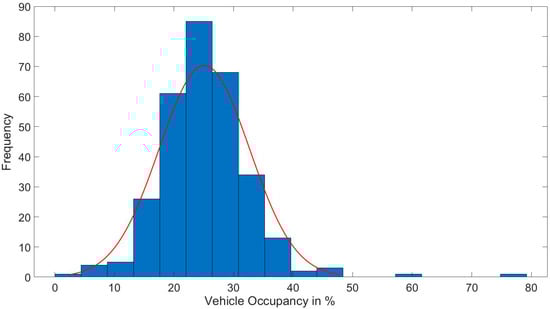
Figure 4.
Frequency distribution of passenger occupancy for all simulated vehicle departures.
From the 304 departures, the occupancy profiles of the mean and high occupancy (the outlier) were selected for further analysis, with and without the effects of passenger mass variation, shown in Figure 5. The selected profiles are of a high and mean passenger occupancy with a constant passenger mass, and mean and high occupancy profiles with passenger mass variation. Figure 5 further shows a change in travel time observed for the different passenger profiles, which is due to the difference in the accumulated dwelling time of the vehicle along the route. These profiles are used as an input for the longitudinal simulation of the powertrain to analyze their influence on the powertrain design.
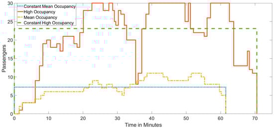
Figure 5.
Mean and high passenger occupancy profiles with/without passenger variation.
2.3. Vehicle Specification and Design Requirements
The inputs for the longitudinal vehicle simulation are the derived speed, slope, and passenger occupancy profiles. The vehicle specification is further required and is provided in Table 1. To ensure that only valid powertrain designs are analyzed from the simulated results, vehicle requirements that the powertrain concept must satisfy are defined. The requirements are shown in Table 1, which include the maximum vehicle speed (r1), gradeability (r2) requirement at the maximum passenger occupancy, acceleration (r3), and range (r4) requirement for the given vehicle specifications [19].

Table 1.
Vehicle requirements and parameters [13].
2.4. Simulation Model for Vehicle Longitudinal Dynamics
The longitudinal vehicle dynamics model calculates the driving resistances of the rolling, aerodynamic, and climbing forces, along with the component efficiencies, to obtain the resulting energy consumption of the vehicle. The derived load profiles of speed, slope, and passenger occupancy are used as an input for the longitudinal simulation.
Using the powertrain design variables of the powertrain architecture, motor power, number of motors, and gears, the initial cost and mass of the powertrain are estimated, which are then used in the longitudinal model to calculate the energy and total costs. The energy consumption calculation uses efficiency maps in the form of load point-dependent look-up tables for the electric motor, inverter, and transmission. The thermal effects are neglected.
Mueller et al. [25] provided a battery model for longitudinal vehicle simulation, as a single cell equivalent circuit model. For the battery design, the number of serial and parallel cells is calculated to achieve the desired battery capacity and voltage level. In the longitudinal simulation, the power load of the whole battery is broken down to a single cell load. Different battery cell types and aging effects are neglected. The cell model is used to calculate the open-circuit voltage, terminal voltage, and internal resistance from the state-of-charge of the cell, which is updated at each time step in the simulation to obtain the resulting power loss of the battery pack.
To simulate the electric motor behavior, an efficiency map of the BMW i3 (Bayerische Motoren Werke AG, Munich, Germany) provided by Kalt et al. [26] is used. To analyze different motor sizes, the torque axis is scaled proportionally to the power, while keeping the efficiency and motor speed constant. The inverter design is coupled to the electric motor. Inverter efficiency map generation is used, which is based on two models developed by Chang for a six-pack IGBT inverter and a MOSFET inverter in a cascaded H-Bridge topology [12]. Depending on the alternative motor design, the inverter map is scaled to the maximum power and maximum speed.
The simulation considers fixed-gear and multi-speed transmissions. The gear ratios of the gearbox are determined using a backwards calculation approach. The required maximum torque and the required maximum speed define the maximum and minimum gear ratio, respectively. The gear step is set to 1.7 to achieve a large total ratio of the transmission. The gear ratio of the final drive and the optional second gear stage are used to derive the desired gear ratio. The effect of the transmission design on the efficiency is considered qualitatively. A base map is created where the efficiency increases linearly from 0% to 100% for partial torques of 0% to 10% of the maximum torque. Furthermore, the efficiency decreases linearly from 100% to 95% for speeds of 0% to 100% of the maximum speed. The number of gears and the possible input torque reduce the maximum efficiency according to an approach by Seeger [27]. For each gear pair, an efficiency map is calculated.
The shift strategy for the gearbox combines the ideas presented by Ngo [28] and Lee et al. [29] for a heuristic energy optimal shift logic. For every load point, the algorithm checks whether a gear shift results in a higher efficiency of the powertrain. In this way, the three areas down shift (I), no shift (II), and up shift (III) are identified, as shown in Figure 6. Figure 6 shows the three areas with respect to the motor speed and the torque. The down shift area is expanded for a low motor speed or high required torques, whereas the up shift area is enlarged at high motor speeds to avoid an operation outside of the feasible operation area.
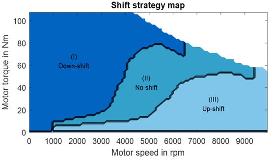
Figure 6.
Shift strategy map.
A powertrain with multiple motors is flexible to distribute the torque request unequally in order to operate the electric machines with less overall losses. This paper only considers different torques at the front and rear axle, while torque vectoring at the same axle is neglected. The model generates a static control map based on the approach proposed by Pesce [10]. For each load point in each possible gear combination, the optimal motor power is determined. Figure 7 shows an example of two 100 kW motors (one at the front axle (Figure 7a) and one at the rear axle (Figure 7b)), with their transmissions in first gear. A higher power is drawn from the front axle motor and the motor is operated alone for low speeds and torques. The rear axle motor serves as a support motor and is only operated alone for high speeds and low torques.
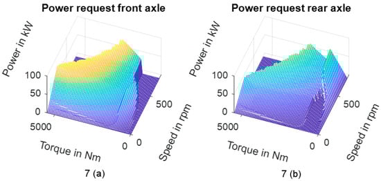
Figure 7.
Example of the motor power distribution between two 100 kW motors in first gear 7 (a) Power request at front axle; 7 (b) Power request at rear axle.
The driver controller is implemented as a Proportional Integral Derivtive (PID) controller. The automatic powertrain design leads to different power to weight ratios of the vehicle and would cause a different sensitivity of the driver for unequal power to weight ratios. Therefore, an inverse vehicle approach, as presented by Matz [9], is implemented. Using a backward calculation, a characteristic map is created that ensures an equal acceleration request by the driver for the same difference in the actual and target speed.
2.5. Energy Consumption Estimation
The model calculates the energy consumption of the defined electric vehicle powertrain concept in Simulink with a forward simulation approach. A predictive motor control unit estimates the power losses using the efficiency maps and determines the power required from the battery to achieve the required target torque. The motor operation strategy demands the power of each motor, as specified in the static control maps. The shift control evaluates whether a shift process leads to a lower energy consumption. Shifting is restricted for the duration of 1 s after a previous shift to avoid shift oscillation. Auxiliary and HVAC power is taken into account as a constant power demand. Energy generation is possible up to the maximum power of the components and is reduced by component power losses. Additional deceleration can be covered by the mechanical braking system at all times and wheel slip is neglected.
The Simulink model allows the simulation of all feasible powertrain structures. In theory, an inverter, a motor, and transmission can be installed. Hence, the model incorporates four subsystems of each component that can be switched on and off, depending on the selected powertrain design. Figure 8 illustrates the six options of the flexible powertrain architecture, which are implemented in MATLAB Simulink. The six architectures, as shown in the figure, are Figure 8a: Base version with one motor at the rear axle, Figure 8b: two rear motors, Figure 8c: booster motor with one rear motor, Figure 8d: booster with two rear motors, Figure 8e: two boosters with one rear motor, and Figure 8f: four motors.
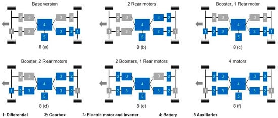
Figure 8.
Variation of powertrain architectures. 8 (a) Base version; 8 (b) 2 Rear motors; 8 (c) Booster, 1 Rear motor; 8 (d) Booster, 2 Rear motors; 8 (e) 2 Boosters, 1 Rear motor; 8 (f) 4 motors.
2.6. Mass and Cost Estimation
The mass of the battery is estimated by the sum of the mass of all cells and a factor to consider wiring and housing. The inverter weight, motor weight, motor inertia, tire weight, and tire inertia are calculated using the regression functions developed by Pesce [10]. The transmission weight and inertia are determined by a program from Seeger [27]. The battery costs are calculated as described in Fries et al. [30]. Inverter, motor, and transmission costs are calculated based on the models suggested by Angerer et al. [16]. The powertrain costs are composed of initial costs and energy costs over the lifetime, according to Equation (4). Table 2 summarizes a description of the symbols and their respective unit and value of the cost calculation.
Table 2.
Description of the symbols, their respective unit, and the value of the cost calculation [19].
2.7. Optimization Framework
An experimental approach is used to find the influence of the powertrain design variation on the vehicle characteristics and to identify the concepts that have the lowest total costs. To create different powertrain designs, the powertrain architecture, motor power, and number of gears are varied for the four different passenger occupancy profiles in Figure 5, which are a constant high passenger occupancy and mean passenger occupancy with and without passenger mass variation. The powertrain architecture is varied between the six powertrain structures provided in Figure 8. The motor power on each axle is varied in 5 kW increments from 20 kW to 240 kW to cover under- and oversized powertrain designs. The transmission for each motor can be a fixed gear, two speeds, or four speeds. The design variation results in a large number of solutions, so further constraints are specified to only simulate feasible concepts. The constraints require the rear axle to always be a driven axle. The minimum combined power of the front and rear axle cannot be less than 160 kW to be able to meet the gradeability requirement. The motor power of the front axle cannot exceed the installed power on the rear axle. The constrained variation leads to a design space of 10,000 unique solutions. Of the solutions created in the design of the experiments, eight design solutions are summarized in Table 3, where the bold letters indicate a modification in comparison to the base version. The base configuration (v1) is the simplest design, which satisfies the performance requirements, as discussed in Table 1. It is defined by a single rear wheel drive with a 240 kW installed power and a fixed gear transmission. The eight selected configurations all have an installed power of 240 kW for comparison.
Table 3.
Selected configurations for a detailed discussion.
The implemented optimization framework allows further design variables to be introduced, such as the battery energy content, the inverter type, and the gear ratio, as well as the shift strategy and the motor power distribution strategy. However, this is beyond the scope of this paper. The powertrain concepts from the design of experiments are simulated and analyzed to understand the influence of the design variation on the costs and vehicle characteristics.
With the design of experiments, the costs and the performance of each derived powertrain concept are obtained. To understand the underlying effects due to the change of the six powertrain architectures in Figure 8 and the multi-speed gearbox of two and four speeds, eight different concepts highlighted in Table 3 are selected for further discussion. The effects of load point shifting and the motor power distribution between the front and rear axle are analyzed to identify the concepts with the lowest total costs. The influence of the passenger occupancy variation on the powertrain design is then discussed.
3. Results
Through the simulation, the powertrain concepts from the design of experiments, the total costs, and the performance of each powertrain concept are calculated. To understand the underlying effects due to the change of the powertrain design, the subsequent subsections discuss the effects on the total costs, the vehicle characteristics, the effects of load point shifting, and the motor power distribution between the front and rear axles. The effects of passenger mass variation and passenger occupancy on the powertrain concept are finally discussed and the optimal solutions of the powertrain concept are presented.
3.1. Effect of Powertrain Architecture Vatiation on the Total Cost
The simulation of four different load profiles with the powertrain design exploration resulted in over 10,000 unique solutions of different powertrain concepts. The influence of the different powertrain architectures and installed powers on the total cost is analyzed in this section. The analysis is based on the six different configurations discussed in Figure 8. Figure 9 shows the cost dependency of installed power for different powertrain architectures. The solutions space is plotted as a box plot figure due to the high number of solutions at each installed power that have different costs. The box plots have a high standard deviation and error bars since they contain the results from the four load profiles and different gear and motor configurations, which results in some solutions having a higher cost at the same installed power. The cost minimum for the solution space is indicated in Figure 9, and the box plots are grouped according to the number of motors and represent the following architectures:
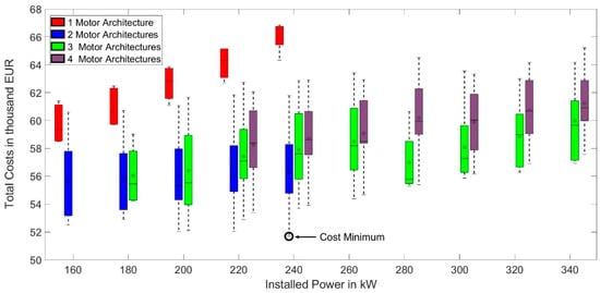
Figure 9.
Cost dependency of installed power for different powertrain architectures.
From Figure 9, it can be deduced that the total costs of the powertrain concept increase with the installed power. The valid solution space for the one-motor configurations is lower in comparison to the two-, three- and four-motor configurations. All the single motor solutions were found to be more expensive in comparison to the other configurations due to their lower energy efficiency and operating costs. The plot consistently displays the advantage of the multiple motor configurations. Although the initial cost of the multiple motor configurations is higher, the configurations prove to be cost-effective. This is due to the lower energy costs during the lifetime. Figure 9 shows that the concepts with two-motor and three-motor configurations with installed power in the range of 200–240 kW are the most cost competitive. The cost minimum indicated is a concept with the booster and one-rear motor architecture with an installed power of 235 kW, and has the lowest total cost of 51,670.23 EUR. The high variation (standard deviation) in total costs for the multi-motor configuration in Figure 9 is caused by the large number of configurations with different motor powers, powertrain architectures, transmission designs, and power distributions. The error bars represent the solutions that result in a high overall efficiency and thus low total costs, as well as solutions that have higher total costs due to incompatible combinations that result in a lower efficiency. Through the powertrain design exploration, the most cost-effective solutions for each architecture can therefore be identified. Figure 9 only provides an overview of the effects of installed power and number of motors on the total costs, and the impacts on the vehicle characteristics and the influence of the transmission, power distribution, and powertrain architecture are discussed in the following sections.
3.2. Effects of Powertrain Architecture Variation on Vehicle Characteristics
Table 1 defines the vehicle parameters and the requirements which the powertrain should satisfy. The requirements include the maximum vehicle speed, gradeability requirement, acceleration, and range. To understand the effect of variation in the powertrain architectures (as shown in Figure 8) on the vehicle characteristics, a radar diagram is used. The radar diagram illustrates the satisfaction of all the vehicle requirements. In addition, it includes the powertrain weight, initial costs, and energy costs. The minimum requirements are set to a value of 1 and the results from different architectures are normalized for comparison. The radar diagram, as shown in Figure 10, has values ranging between 0.5 and 1.5. The concepts that do not meet certain requirements have a value of less than 1. Some values exceed 1.5, but are set to be displayed as 1.5 for better visualization. For comparing other properties, including the powertrain weight, initial costs, and energy costs, the base version parameters are used as a reference and are normalized to 1.
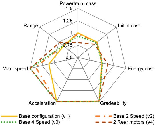
Figure 10.
Vehicle characteristics of versions 1–4.
The base version (v1) is the simplest design that meets all the requirements. It is defined by a single rear wheel drive with a 240 kW installed power and a fixed gear transmission. The powertrain weight accounts for 1186 kg, where the battery weighs 941 kg, the inverter weighs 26 kg, the motor weighs 54 kg, and the transmission weighs 59 kg. The cost estimation shows that the initial cost is 19,320 EUR, of which the battery costs 15,104 EUR. The energy consumption cost over the lifetime is 47,530 EUR. The seven selected configurations all have an installed power of 240 kW for comparison. Therefore, the configurations are considered better in comparison if the individual values exceed 1.
3.2.1. Rear Wheel Drive Powertrain Configuration
Figure 10 compares the vehicle characteristics of the base version (v1) and the three variations (v2–v4) that are rear wheel-driven. All the configurations meet the gradeability, acceleration, and speed requirements, with values greater than 1. However, none of the powertrain designs are able to meet the minimum range requirement. Figure 10 shows that the v4 configuration has the lowest powertrain mass rating (0.80) and initial cost rating (0.93). This is because an increase in the number of motors and inverters leads to an increase in the initial cost and powertrain mass. However, the v4 configuration has the lowest energy cost (value of 1.13). Hence, v4 with an energy cost of 42,191 EUR is the best rear axle design, compared to the three other variations (v1–v3).
3.2.2. All-Wheel Powertrain Configuration
Figure 11 illustrates the vehicle characteristics for the five configurations comparing v1 with four other configuration (v5–v8) that are all-wheel-driven. It can be seen that all the configurations meet the gradeability, acceleration, speed, and range requirements. The powertrain mass of the all-wheel powertrain designs is heavier compared to the base version, with the concept with four motors (v8) being the heaviest. In addition, v1 has the lowest initial costs. This is again due to the lower number of components of the powertrain. However, as seen from Figure 9, v1 has the highest energy cost when compared to all the other configurations.
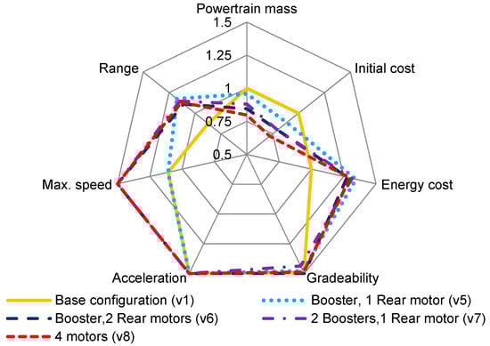
Figure 11.
Vehicle characteristics of versions 1 and 5–8.
To summarize, all the four-wheel drive concepts display a much lower energy consumption than the base version (v1) and the entire rear wheel drive configurations (v2–v4). The v5 configuration with a booster and one rear motor is the best solution in terms of the economical rating in comparison to all the eight concepts and satisfies all the simulation requirements.
3.3. Load Point Shifting (Transmission and Motor)
The change in powertrain configuration due to the variation of motor size, number of gears, and the change in powertrain architecture strongly influences the operating points on the combined efficiency map. Figure 12 compares the load points and resulting efficiency of three powertrain configurations of the base version (v1), base version with a multi-speed gearbox (v3), and a four-wheel drive configuration (v5), to illustrate the processes of load point shifting in detail.
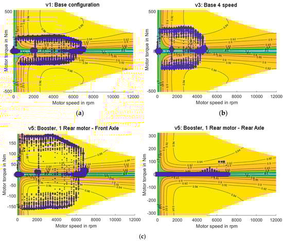
Figure 12.
Load point shifting by transmission (a) v1 configuration with fixed gear (b) 4 speed configuration (c) v5 Booster configuration.
Figure 12a shows the efficiency map and load points of the base version (v1). It can be seen that the majority of load points on the efficiency map are below the peak efficiency region as the gear ratio for a single speed gearbox is designed for the maximum torque requirement, which results in the load points occurring in a lower region of efficiency.
Figure 12b compares the four-speed transmission concept (v3) of the powertrain against the base version. The four-speed transmission has a higher overall efficiency compared to the base version (v1), as some of the operating points are moved to a higher efficiency level with the additional gear ratios; however, the concept fails to precisely find the peak efficiency area most of the time. In addition, some combinations of the multi-speed gearbox architecture even resulted in higher losses, despite the increased flexibility to select a load point, because of the higher number of gears and the increased mass of the transmission system.
The four-wheel drive configurations (v5) with the additional small motor at the front axle (v5) were found to be the most effective method to move the operating points to a higher region of efficiency. The four-wheel configuration distributes the load between the two motors and optimizes their operation. As seen in Figure 12c, the booster motor in the front axle is often sufficient to meet the requested power alone. The rear axle motor only provides additional torque when the required torque exceeds the maximum torque of the front motor. Furthermore, the load points are more often located in an area of high efficiency and even reach the maximum at times, as shown in Figure 12c. A high flexibility for choosing the load point between the motors proves to be an effective measure to reduce the energy consumption and overall costs.
3.4. Effects of Motor Power Distribution
The four-wheel drive architecture with the booster and one-rear motor configuration is shown to be effective to move the operational points to a higher efficiency region. Another important aspect is to understand the effects of the power distribution between the front axle and the rear axle and the effects of a multi-speed gear configuration that would influence the load points. Figure 13 shows the cost dependency of the motor power distribution between the front and rear axle. The single, two-speed, and four-speed gearbox configurations are considered for powertrain concepts with an installed power of 240 kW. Figure 13 shows that the concepts with fixed speed gear configurations have the lowest cost, which decreases to an optimum power distribution of 36% of installed power at the front axle. Similarly, the two-speed and four-speed gear configurations also showed the trend of decreasing costs at an optimal power distribution of 46% and 40%, respectively. Therefore, a booster and one-rear motor configuration with a fixed transmission would be an ideal powertrain architecture.
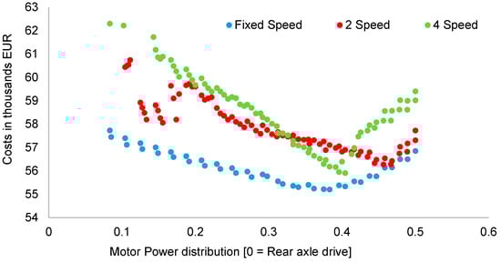
Figure 13.
Cost dependency of motor power distribution.
3.5. Influence of Passenger Mass Variation and Occupancy
Lastly, the influence of passenger occupancy on the powertrain concept is investigated. Out of all the valid solutions, Table 4 shows the top five concepts in terms of the total cost for the four different passenger occupancy profiles. The table shows different passenger loads; motor topologies; and the respective motor power, transmission, energy cost, and the total cost in Euros. As discussed in the previous section, the most cost-competitive architecture is the concept with the booster and one-rear motor configuration (Figure 8c) with fixed gear transmission. In addition, the total installed power ranges between 235 and 240 kW. From the four load profiles simulated, no concepts with a two-motor configuration at each of the front and/or rear axles achieved a total cost lower than the concepts listed in Table 4.
Table 4.
Five best cost-competitive configurations for different passenger loads.
The mean occupancy with and without passenger variation precisely has the same five best concepts. The energy costs of the concepts vary because of the difference in the passenger load. The high occupancy with a constant number of passengers has a similar power distribution. However, due to a constant high passenger load, this profile has the highest energy cost and hence total cost. The high occupancy with passenger variation has a different motor power distribution compared to the other three passenger load profiles. Since the passenger loading in this profile reaches up to 100%, the front axle motor size is increased to optimize the operational points of the two motors. Therefore, the change in the passenger load profile does not influence the ideal powertrain architecture. However, the power distribution changes to compensate for the variation in load.
4. Summary and Conclusions
This paper has presented a holistic powertrain design optimization framework for electric city buses by using realistic load profiles. Six different powertrain architectures with different numbers of gears and installed powers were investigated to determine their impacts on vehicle characteristics and total costs using realistic load profiles. In addition, the effects of passenger occupancy and passenger variation on the powertrain concept were investigated.
The developed simulation framework is capable of investigating the variation in component types, component sizes, and powertrain architectures. The methodology uses regression models to estimate the component weights and initial powertrain component costs. An equivalent circuit model, along with component efficiency maps for the motor, inverter, and transmission, are used in the energy consumption simulation and energy optimized static maps for the control strategy of the motor power distribution and shift process. The model can investigate the underlying effects of powertrain design decisions, such as the motor type, installed power, powertrain architecture, and number of gears, on the energy consumption, vehicle characteristics, and total costs.
The results of the paper showed the single rear motor configuration to be the least cost-effective, despite having the lowest acquisition costs. Multiple motor and multi-speed transmission configurations were further analyzed. Solutions with multiple gears were found to shift the operating load points to a higher efficiency region, but failed to find the peak efficiency operating point for most powertrain concepts. The load point shifting with multiple motors was found to be an effective method to increase the overall powertrain efficiency, which resulted in solutions with the lowest total costs. The power distribution between the front and rear axles was further found to influence the efficiency of the multi-motor powertrain architecture. The powertrain efficiency improves with increasing power split until an optimum, after which the efficiency degrades. Furthermore, the fixed speed gearbox for multiple motor configurations was found to have a higher efficiency compared to multi-speed gearboxes for multiple motors. In summary, multiple motor configurations were found to have better vehicle characteristics of maximum speed, acceleration, and top speed, in addition to lower energy costs, in comparison to the single rear motor configuration.
The effects on the powertrain design due to occupancy and passenger mass variation were investigated by simulating the passenger arrival process in combination with a fleet simulation to obtain the load profiles of mean passenger occupancy with and without a constant passenger mass, and a high passenger occupancy with and without a constant passenger mass. For the mean passenger occupancy, there was no influence on the powertrain concept with the variation of passenger mass. The high passenger occupancy with mass variation resulted in a different optimal powertrain concept; however, the architecture and total motor power remained constant.
Further research is required to refine parts of the method, such as the automated transmission design and the control strategies. Including battery aging costs and the maintenance costs may lead to a more realistic cost prediction. Additional design variables, such as the gear step of the transmission and the battery energy content, as well as a finer step size for the installed power, may lead to further improvement of the powertrain costs over the lifetime. However, a larger solution space increases the computational time and may make the application of optimization heuristics, such as genetic algorithms, necessary.
Author Contributions
The first two authors A.P. and G.S. contributed equally to this work. A.P. and S.K. predominantly accomplished the conceptualization, methodology, and simulations. Data curation, formal analysis, and validation were mainly accomplished by G.S., A.P. and G.S. contributed to writing/preparing the original draft. A.O. contributed to the project administration and review/editing. M.L. gave final approval of the version to be published and agreed to all aspects of the work. As a guarantor, he accepts responsibility for the overall integrity of the paper.
Funding
This work was financially supported by the Singapore National research Foundation (NRF) under its Campus for Research Excellence and Technological Enterprise (CREATE) program.
Acknowledgments
We would like to acknowledge the support of Christian Angerer during the development of the longitudinal model, as well as that of Alexander Koch and Olaf Teichert for the derivation of the speed and slope profiles.
Conflicts of Interest
The authors declare no conflict of interest.
References
- Cooney, G.; Hawkins, T.R.; Marriott, J. Life Cycle Assessment of Diesel and Electric Public Transportation Buses. J. Ind. Ecol. 2013, 451. [Google Scholar] [CrossRef]
- Ercan, T.; Zhao, Y.; Tatari, O.; Pazour, J.A. Optimization of transit bus fleet’s life cycle assessment impacts with alternative fuel options. Energy 2015, 93, 323–334. [Google Scholar] [CrossRef]
- Zhou, B.; Wu, Y.; Zhou, B.; Wang, R.; Ke, W.; Zhang, S.; Hao, J. Real-world performance of battery electric buses and their life-cycle benefits with respect to energy consumption and carbon dioxide emissions. Energy 2016, 96, 603–613. [Google Scholar] [CrossRef]
- Berthold, K.; Förster, P.; Rohrbeck, B. Location Planning of Charging Stations for Electric City Buses. In Operations Research, Proceedings of the International Conference of the German, Austrian and Swiss Operations Research Societies (GOR, ÖGOR, SVOR/ASRO), University of Vienna, Austria, 1–4 September 2015; Doerner, K., Ljubic, I., Pflug, G., Tragler, G., Eds.; Springer: Cham, Switzerland, 2017; pp. 237–242. ISBN 978-3-319-42901-4. [Google Scholar]
- Fusco, G.; Alessandrini, A.; Colombaroni, C.; Valentini, M.P. A Model for Transit Design with Choice of Electric Charging System. Procedia Soc. Behav. Sci. 2013, 87, 234–249. [Google Scholar] [CrossRef][Green Version]
- Gao, Z.; Lin, Z.; LaClair, T.J.; Liu, C.; Li, J.-M.; Birky, A.K.; Ward, J. Battery capacity and recharging needs for electric buses in city transit service. Energy 2017, 122, 588–600. [Google Scholar] [CrossRef]
- Pihlatie, M.; Kukkonen, S.; Halmeaho, T.; Karvonen, V.; Nylund, N.-O. Fully electric city buses—The viable option. In IEVC, Proceedings of the IEEE International Electric Vehicle Conference, Palazzo dei Congressi, Florence, Italy, 17–19 December 2014; IEEE: New York, NY, USA, 2015; pp. 1–8. ISBN 978-1-4799-6075-0. [Google Scholar]
- Kuchenbuch, K.; Vietor, T.; Stieg, J. Optimisation Algorithms for the Design of Electric Cars. ATZ Worldw. 2011, 113, 16–19. [Google Scholar] [CrossRef]
- Matz, S. Nutzerorientierte Fahrzeugkonzeptoptimierung in einer multimodalen Verkehrsumgebung. Ph.D. Thesis, Technical University Munich, Munich, Germany, 2015. [Google Scholar]
- Pesce, T. Ein Werkzeug zur Spezifikation von effizienten Antriebstopologien für Elektrofahrzeuge. Ph.D. Thesis, Technical University Munich, Munich, Germany, 2014. [Google Scholar]
- Schönknecht, A.; Babik, A.; Rill, V. Electric Powertrain System Design of BEV and HEV Applying a Multi Objective Optimization Methodology. Transp. Res. Procedia 2016, 14, 3611–3620. [Google Scholar] [CrossRef]
- Chang, F.; Ilina, O.; Hegazi, O.; Voss, L.; Lienkamp, M. Adopting MOSFET multilevel inverters to improve the partial load efficiency of electric vehicles. In Proceedings of the 19th European Conference on Power Electronics and Applications (EPE’17 ECCE Europe), Warsaw, Poland, 11–14 September 2017; pp. 1–13. [Google Scholar]
- Ghanaatian, M.; Radan, A. Modeling and simulation of Dual Mechanical Port machine. In Proceedings of the 4th Power Electronics, Drive Systems & Technologies Conference (PEDSTC), Tehran, Iran, 13–14 February 2013; pp. 125–129, ISBN 978-1-4673-4484-5. [Google Scholar]
- Ghanaatian, M.; Radan, A. Application and simulation of dual-mechanical-port machine in hybrid electric vehicles. Int. Trans. Electr. Energ. Syst. 2015, 25, 1083–1099. [Google Scholar] [CrossRef]
- Liu, Y.; Niu, S.; Ho, S.L.; Fu, W.N. A New Hybrid-Excited Electric Continuous Variable Transmission System. IEEE Trans. Magn. 2014, 50, 1–4. [Google Scholar] [CrossRef]
- Angerer, C.; Krapf, S.; Buß, A.; Lienkamp, M. Holistic Modeling and Optimization of Electric Vehicle Powertrains Considering Longitudinal Performance, Vehicle Dynamics, Costs and Energy Consumption. In Proceedings of the ASME 2018 International Design Engineering Technical Conferences and Computers and Information in Engineering Conference, Quebec City, QC, Canada, 26–29 August 2018. [Google Scholar]
- Fries, M.; Lehmeyer, M.; Lienkamp, M. Multi-criterion optimization of heavy-duty powertrain design for the evaluation of transport efficiency and costs. In Proceedings of the 20th International Conference on Intelligent Transportation Systems (ITSC), Yokohama, Japan, 16–19 October 2017; pp. 1–8. [Google Scholar]
- Lajunen, A. Comparison of Different Powertrain Configurations for Electric City Bus. In 2014 IEEE Vehicle Power and Propulsion Conference (VPPC), Proceedings of the 2014 IEEE Vehicle Power and Propulsion Conference (VPPC), Coimbra, Portugal, 27–30 October 2014; IEEE: Piscataway, NJ, USA, 2014; pp. 1–5. ISBN 978-1-4799-6783-4. [Google Scholar]
- Krapf, S.; Sethuraman, G.; Pathak, A.; Ongel, A.; Lienkamp, M. Improving electric city bus powertrain efficiency and costs using design space exploration. In Proceedings of the EVS 31 & EVTeC 2018, Kobe, Japan, 1–3 October 2018. [Google Scholar]
- Koch, A.; Teichert, O.; Kalt, S.; Ongel, A.; Lienkamp, M. Powertrain optimization for autonomous buses under optimal speed control. Energy 2019. (under review). [Google Scholar]
- Farr, T.G.; Rosen, P.A.; Caro, E.; Crippen, R.; Duren, R.; Hensley, S.; Kobrick, M.; Paller, M.; Rodriguez, E.; Roth, L.; et al. The Shuttle Radar Topography Mission. Rev. Geophys. 2007, 45, 1485. [Google Scholar] [CrossRef]
- Li, B. Markov models for Bayesian analysis about transit route origin–destination matrices. Transp. Res. Part B Methodol. 2009, 43, 301–310. [Google Scholar] [CrossRef]
- Land Transport Authority. TransitLink eGuide—Bus Enquiry. Available online: https://www.transitlink.com.sg/eservice/eguide/service_route.php?service=15 (accessed on 2 August 2019).
- Sun, L.; Tirachini, A.; Axhausen, K.W.; Erath, A.; Lee, D.-H. Models of bus boarding and alighting dynamics. Transp. Res. Part A Policy Pract. 2014, 69, 447–460. [Google Scholar] [CrossRef]
- Müller, S.; Rohr, S.; Schmid, W.; Lienkamp, M. Analysing the Influence of Driver Behaviour and Tuning Measures on Battery Aging and Residual Value of Electric Vehicles. In Proceedings of the Electric Vehicle Symposium 30 (EVS30), Stuttgart, Germany, 9–11 October 2017. [Google Scholar]
- Kalt, S.; Erhard, J.; Danquah, B.; Lienkamp, M. Electric Machine Design Tool for Permanent Magnet Synchronous Machines. In 2019 Fourteenth International Conference on Ecological Vehicles and Renewable Energies (EVER), Proceedings of the 2019 Fourteenth International Conference on Ecological Vehicles and Renewable Energies (EVER), Monte-Carlo, Monaco, 8–10 May 2019; IEEE: Piscataway, NJ, USA, 2019; pp. 1–7. ISBN 978-1-7281-3703-2. [Google Scholar]
- Seeger, F. Energetische Modellierung verschiedener Systeme zur Momentenverteilung für ein adaptives Antriebsstrangmodell. Semester Thesis, Technical University Munich, Munich, Germany, 2017. [Google Scholar]
- Ngo, D.V. Gear shift strategies for automotive transmissions. Ph.D. Thesis, Eindhoven University of Technology, Eindhoven, The Netherlands, 2012. [Google Scholar]
- Lee, T.; Kim, Y.; Nam, K. Loss minimizing gear shifting algorithm based on optimal current sets for IPMSM. In Proceedings of the 2017 IEEE Transportation Electrification Conference and Expo (ITEC), Chicago, IL, USA, 22–24 June 2017; pp. 135–140. [Google Scholar]
- Fries, M.; Kerler, M.; Rohr, S.; Sinning, M.; Schickram, S.; Lienkamp, M.; Kochhan, R.; Fuchs, S.; Reuter, B.; Burda, P.; et al. An Overview of Costs for Vehicle Components, Fuels, Greenhouse Gas. Emissions and Total Cost of Ownership—Update 2017; researchgate.com: Berlin, Germany, 2017. [Google Scholar]


© 2019 by the authors. Licensee MDPI, Basel, Switzerland. This article is an open access article distributed under the terms and conditions of the Creative Commons Attribution (CC BY) license (http://creativecommons.org/licenses/by/4.0/).