Ensemble of Networks for Multilabel Classification

Abstract

Multilabel learning goes beyond standard supervised learning models by associating a sample with more than one class label. Among the many techniques developed in the last decade to handle multilabel learning best approaches are those harnessing the power of ensembles and deep learners. This work proposes merging both methods by combining a set of gated recurrent units, temporal convolutional neural networks, and long short-term memory networks trained with variants of the Adam optimization approach. We examine many Adam variants, each fundamentally based on the difference between present and past gradients, with step size adjusted for each parameter. We also combine Incorporating Multiple Clustering Centers and a bootstrap-aggregated decision trees ensemble, which is shown to further boost classification performance. In addition, we provide an ablation study for assessing the performance improvement that each module of our ensemble produces. Multiple experiments on a large set of datasets representing a wide variety of multilabel tasks demonstrate the robustness of our best ensemble, which is shown to outperform the state-of-the-art.

1. Introduction

Multilabel learning extends the standard supervised learning model that associates a sample with a single label by simultaneously categorizing samples with more than one class label. In the past, multilabel learning has been successfully implemented in many different domains [1], such as bioinformatics [2,3,4], information retrieval [5,6], speech recognition [7,8], and online user reviews with negative comment classification [9,10].

As proposed by various researchers, one of the most intuitive handlings of multilabel classification is to treat it as a series of independent two-class binary classification problems, known as Binary Relevance (BR) [11,12]. However, this approach has several limitations: the performance is relatively poor; it lacks scalability; and it cannot retain label correlations. Researchers have tried improving these issues using chains of binary classifiers [13], feature selections [14,15,16], class dependent and label specific features [17], and data augmentation [5]. Among these investigations, the augmentation method in [5] has demonstrated the best performance on some multilabel datasets using Incorporating Multiple Cluster Centers (IMCC). In biomedical datasets, hML-KNN [18] has also proven to be one of the best multilabel classifiers, its success relying on feature-based and neighbor-based similarity scores.

Generating ensembles of classifiers is yet another robust and dependable method for enhancing performance on multilabel data [15,19], with bagging shown to perform well in several multilabel classification benchmarks [20,21]. However, a common problem in bagging is pairwise label correlation. To solve this problem, [22] invented a stacking technique where learners were trained on each label. The decisions of the classifiers were fed into stacked combinations combined with a meta-level classifier whose output produced a final decision. Another algorithm of note is the RAndom k-labELsets (RAkEL) [19], which constructed ensembles by training single-label learning models on random subsets of labels. The reader is referred to [23,24] for a discussion of some recent RAkEL variants.

Rather quickly, multilabel systems incorporating deep learners have risen to the top in classification performance. The impact deep learning has had on this field is visible in the large number of open source and commercial APIs currently providing deep learning solutions to multilabel classification problems. Some open source APIs are DeepDetect [25], VGG19 (VGG) [26], Inception v3 [27], InceptionResNet v2 [28], ResNet50 [29], MobileNet v2 [30], YOLO v3 [31], and fastai [32]. Some of the commercially available APIs include Imagga [33], Wolfram Alpha’s Image Identification [34], Clarifai [35], Microsoft’s Computer Vision [36], IBM Watson’s Visual Recognition [37], and Google’s Cloud Vision [38]. A comparison of performance across several multilabel benchmarks is reported in [39].

Despite these advances in deep multilabel learning, research using advanced techniques, including those for building ensembles, has lagged compared to work in other areas of machine learning. The few ensembles that have been built for multilabel problems apply simple techniques (we describe the state of the art in Section 2). More innovative ensembling techniques have yet to be explored. The most advanced is proposed in [9], where random forest [40] was used as the ensembling technique. Only a couple of studies have explored ensembling with deep learners [2,41]. There is a need to investigate cutting edge deep learning ensembling methods for the multilabel problem.

The goal of this paper is to experimentally derive a more advanced ensemble for multilabel classification that combines Long Short-Term Memory networks (LSTM) [42], GRU [43], and Temporal Convolutional Neural Networks (TCN) [44] using Adam variants [45] as the means of ensuring diversity. We posted some early preliminary results combining these classifiers on ArXiv [46]. Conceptually, a GRU is a simplified Bidirectional Long Short-Term Memory (LSTM) model. GRU and LSTM have hidden temporal states and gating mechanisms. Both networks have a problem with intermediate activations, a function of low-level features. To offset this shortcoming, these models must be combined with classifiers that discern high-level relationships. In the research presented here, we investigate the potential of TCN as a complement classifier since it offers the advantage of hierarchically capturing relationships across high, intermediate, and low-level timescales.

As mentioned, diversity in ensembles composed of LSTM, GRU, and TCN is assured in our approach by incorporating different Adam optimization variants. Adam finds low minima of the training loss, and many variants have been developed for augmenting Adam’s strengths and offsetting its weaknesses. As will be demonstrated, combining ensembles of LSTM, GRU, and TCN with IMCC [5] and a bootstrap-aggregated (bagged) decision trees ensemble (TB) [9] (carefully modified for managing multilabel data) further enhances performance.

Some of the contributions of this study are the following:

• To the best of our knowledge, we are the first to propose an ensemble method for managing multilabel classification based on combining sets of LSTM, GRU, and TCN, and we are the first to use TCN on this problem.
• Two new topologies of GRU and TCN are also proposed here, as well as a novel topology that combines the two.
• Another advance in multilabel classification is the application of variants of Adam optimization for building our ensembles.
• Finally, for comparison with future works by other researchers in this area, the MATLAB source code for this study is available at https://github.com/LorisNanni (accessed on 1 November 2022).

The effectiveness and strength of investigating more cutting-edge ensembling techniques are demonstrated in the experimental section where we evaluate the performance of different ensembles with some baseline approaches across several multilabel benchmarks. Our best deep ensemble is compared with the best multilabel methods tested to date and shown to obtain state-of-the-art performance across many domains.

This paper is organized as follows: In Section 2, we report on some recent work applying deep learning to multilabel classification. In Section 3 we describe the benchmarks and performance indicators used in the experimental section. In Section 4, each element and pre-processing in the proposed approach is detailed. This section covers a brief discussion of the preprocessing methods used and descriptions of GRU, TCN, IMCC, and LSTM networks. This section also describes pooling, training, and our method for generating the ensembles. In Section 5, Adam optimization and all the Adam variants tested here are addressed. In Section 6, experimental results are presented and discussed. Finally, in Section 7, we summarize the results and outline some future directions of research.

2. Related Works

One of the first works to apply deep learning to the problem of multilabel classification is [47]. The authors in that study proposed a simple feed-forward network using gradient descent to handle the functional genomics problem in computational biology. A growing body of research has since ensued that has advanced the field and application of deep learning to a wide range of multilabel problems. In [48], for example, a Convolutional Neural Network (CNN) combined with data augmentation using binary cross entropy (BCE) loss and adagrad optimization was designed to tackle the problem of land cover scene categorization. In [49], a CNN using multiclass cross entropy loss was developed to detect heart rhythm/conduction abnormalities. In that study, each element in the output vector corresponded to a rhythm class. An early ensemble was developed in [50], that combined CNN with LSTM to handle the multilabel classification problem of protein-lncRNA interactions, and in [2] an ensemble of LSTM combined with an ensemble of classifiers based on Multiple Linear Regression (MLR) was generated to predict a given compound’s Anatomical Therapeutic Chemical (ATC) classifications. Recurrent CNNs (RCNNs) have recently been evaluated in many multilabel problems, including identifying surgical tools in laparoscopic videos [51] using a GRU and in recommendation systems for prediagnosis support [52].

A growing number of researchers, in addition to [51], have explored the benefits of adding GRUs to enhance the performance of multilabel systems. In [53], for example, sentiment in tweets were analyzed by extracting topics with a C-GRU (Context-aware GRU). a sentiment in tweets were analyzed by extracting topics with a C-GRU (Context-aware GRU). In [54], a classifier system called NCBRPred was designed with bidirectional GRUs (BiGRUs) to predict nucleic acid binding residues based on the multilabel sequence labeling model. The BiGRUs were selected to capture the global interactions among the residues.

In terms of ensembles built to handle multilabel problems, GRUs have been shown to work well with CNNs. In [41], an Inception model using was combined with GRU network to identify nine classes of arrhythmias. Adam was used for optimization in [41], but no variants were used for building ensembles as in the system proposed here.

Table 1. Summary of existing deep learning studies. An X indicates whether a particular technique or model was used.

	[47]	[48]	[49]	[50]	[2]	[51]	[52]	[53]	[54]	[41]	[9]	Here
Ensemble					X					X	X	X
GRU						X		X	X	X		X
CNN		X	X	X		X	X
LSTM				X	X							X
TCN												X
RNN							X
Inception model										X
Random forest											X	X
Gradient descend	X									X
Stochastic gradient descend						X	X
Data augmentation		X		X		X			X
Multiple loss functions								X
Binary cross entropy (BCE) loss		X						X	X	X		X
Multiclass cross entropy loss			X
Logistic regression								X
Multiple linear regression					X
Quantile regression											X	X
Various optimization methods	X
Adagrad optimization		X
Variants of Adam optimization									X	X		X

compares existing models for deep learning, as discussed above, applied to the multilabel problem. The first column lists the techniques and models used in these systems and indicates whether ensembles were used in the study. An X means that the indicated technique or model was used.

3. DataSets

The following multilabel data sets were selected to evaluate our approach. These are standard benchmarks in multilabel research and run the gamut of typical multilabel problems (music, image, biomedical, and drug classifications). The names provided below are not necessarily those reported in the original papers but rather those commonly used in the literature.

• Cal500 [55]: This dataset contains human-generated annotations, which label some popular Western music tracks. Tracks were composed by 500 artists. Cal500 has 502 instances, including 68 numeric features and 174 unique labels.
• Scene [11]: This dataset contains 2407 color images. It includes a predefined training and testing set. The images can have the following labels: beach (369), sunset (364), fall foliage (360), field (327), mountain (223), and urban (210). Sixty-three images have been assigned two category labels and one image three, making the total number of labels fifteen. The images all went through a preprocessing procedure. First, the images were converted to the CIE Luv space, which is perceptually uniform (close to Euclidean distances). Second, the images were divided into a 7 × 7 grid, which produced 49 blocks. Third, the mean and variance of each band were computed. The mean represents a low-resolution image, while the variance represents computationally inexpensive texture features. Finally, the images were transformed into a feature vector (49 × 3 × 2 = 294 dimensions).
• Image [56]: This dataset contains 2000 natural scene images. Images are divided into five base categories: desert (340 images), mountains (268 images), sea (341 images), sunset (216 images), and trees (378 images). Categorizing images into these five basic types produced a large dataset of images that belonged to two categories (442 images) and a smaller set that belonged to three categories (15 images). The total number of labels in this set, however, is 20 due to the joint categories. All images went through similar preprocessing methods as discussed in [11].
• Yeast [57]: This dataset contains biological data. In total there are 2417 micro-array expression data and phylogenetic profiles. They are represented by 103 features and are classified into 14 classes based on function. A gene can be classified into more than one class.
• Arts [5]: This dataset contains 5000 art images, which are described by a total of 462 numeric features. Each image can be classified into 26 classes.
• Liu [15]: This dataset contains drug data used to predict side effects. In total it has 832 compounds. They are represented by 2892 features and 1385 labels.
• ATC [58]: This dataset contains 3883 ATC coded pharmaceuticals. Each sample is represented by 42 features and 14 classes.
• ATC_f: This dataset is a variation of the ATC data set described above. In this dataset, however, the patterns are represented by a descriptor of 806 dimensions (i.e., all three descriptors are examined in this dataset as described in [59]).
• mAn [4]: This dataset contains protein data represented by 20 features and 20 labels.
• Bibtex: This dataset is highly sparse and was used in [5].
• Enron: a highly sparse dataset used in [5].
• Health: a highly sparse dataset used in [5].

Table 2. Datasets summary.

Name	#Patterns	#Features	#Labels	LCard
CAL500	502	68	174	26.044
Image	2000	294	5	1.236
Scene	2407	294	5	1.074
Yeast	2417	103	14	4.24
Arts	5000	462	26	1.636
ATC	3883	42	14	1.265
ATC_f	3883	700	14	1.265
Liu	832	2892	1385	71.160
mAn	3916	20	20	1.650
bibtex	7395	1836	159	2.402
enron	1702	1001	53	3.378
health	5000	612	32	1.662

shows a summary of the benchmarks along with their names, number of patterns, features, and labels, as well as the average number of class labels per pattern (LCard).

For dataset 6 (Liu), a 5-fold cross-validation testing protocol is used, and the results are averaged. For datasets 7 to 9, a 10-fold protocol is used. Datasets 1–5 and 10–12 are in the MATLAB IMCC toolkit [5]. Available at https://github.com/keauneuh/Incorporating-Multiple-Cluster-Centers-for-Multi-Label-Learning/tree/master/IMCCdata (accessed on 24 September 22). All other datasets can be obtained from the references provided in their description above.

Performance Indicators

In the experimental section, several performance indicators are used to evaluate the classifiers on the multiclass benchmarks.

Let X be a dataset with m samples ${\mathit{x}}_i\in {\Re }^d$. A given sample has an actual label ${\mathbf{y}}_i \in {\left\{0, 1\right\}}^l$, where l is the number of total labels. Let H and F be the set of predicted labels, where ${\mathit{h}}_i \in {\left\{0, 1\right\}}^l$ is the predicted label vector for sample ${\mathit{x}}_i$, and ${\mathit{f}}_i\in {\Re }^l$ is the confidence relevance of each prediction. The performance indicators are defined for H and F as follows:

• Hamming loss is the fraction of misclassified labels,

  $$\mathrm{HLoss}\left(H\right)=\frac{1}{ml}{\displaystyle \sum }_{i=1}^m{\displaystyle \sum }_{j=1}^{l}I\left({\mathbf{y}}_i\left(j\right)\ne {\mathit{h}}_i\left(j\right)\right) ,$$

  (1)

  where I() is the indicator function. Hamming loss must be minimized. When hamming loss is 0, there is no error in the predicted label vector.
• One error is the fraction of instances whose most confident label is incorrect. The indicator should be minimized:

  $$\mathrm{OneError}\left(\mathrm{F}\right)=\frac{1}{m}{\displaystyle \sum }_{i=1}^{m}I\left({\mathit{h}}_i\left(\underset{j}{\mathrm{argmax}}{\mathit{f}}_i\right) \ne {\mathbf{y}}_i\left(\underset{j}{\mathrm{argmax}}{\mathit{f}}_i\right) \right) ,$$

  (2)
• Ranking loss is the average fraction of reversely ordered label pairs for each instance. It is derived from the confidence value by taking into account the number of confidence values correctly ranked (i.e., when a true label is ranked before a wrong label). Ranking loss is also an error. Therefore, it should be minimized.
• Coverage is the average number of steps needed to move down the ranked label list of an instance to cover all its relevant labels. As such, coverage should be minimized.
• Average precision is the average fraction of relevant labels ranked higher than a particular label. As such, average precision should be maximized.

Another set of indicators adopted by many researchers [60]:include:

• Aiming is the ratio of correctly predicted labels and practically predicted labels:

  $$\mathrm{Aiming}\left(H\right)=\frac{1}{m}{\displaystyle {\sum }_{i=1}^m}\frac{\left|\right|{\mathit{h}}_i{\displaystyle \cap }{\mathbf{y}}_i\left|\right|}{\left|\right|{\mathit{h}}_i\left|\right|}$$

  (3)
• Recall is the rate of the correctly predicted labels and actual labels:

  $$\mathrm{Recall}\left(H\right)=\frac{1}{m}{\displaystyle {\sum }_{i=1}^m}\frac{\left|\right|{\mathit{h}}_i\cap {\mathbf{y}}_i\left|\right|}{\left|\right|{\mathbf{y}}_i\left|\right|} .$$

  (4)
• Accuracy is the average ratio of correctly predicted labels over total labels:

  $$\mathrm{Accuracy}\left(H\right)=\frac{1}{m}{\displaystyle {\sum }_{i=1}^m}\frac{\left|\right|{\mathit{h}}_i\cap {\mathbf{y}}_i\left|\right|}{\left|\right|\mathit{h}\cup {\mathbf{y}}_i\left|\right|}.$$

  (5)
• Absolute true is the ratio of the perfectly correct prediction events and the total number of prediction events:

  $$\mathrm{AbsTrue}\left(H\right)=\frac{1}{m}{\displaystyle {\sum }_{i=1}^m}I\left({\mathit{h}}_i={\mathbf{y}}_i\right) .$$

  (6)
• Absolute false is the ratio of the completely wrong prediction events and total number of prediction events:

  $$\mathrm{AbsFalse}\left(H\right)=\frac{1}{m}{\displaystyle {\sum }_{i=1}^m}\frac{\left|\right|{\mathit{h}}_i\cup {\mathbf{y}}_i\left|\right|-\left|\right|{\mathit{h}}_i\cap {\mathbf{y}}_i\left|\right|}{l} .$$

  (7)

All ten indicators lie within the range [0, 1] and should be maximized, except for Absolute false.

4. Proposed Approaches

4.1. Model Architectures

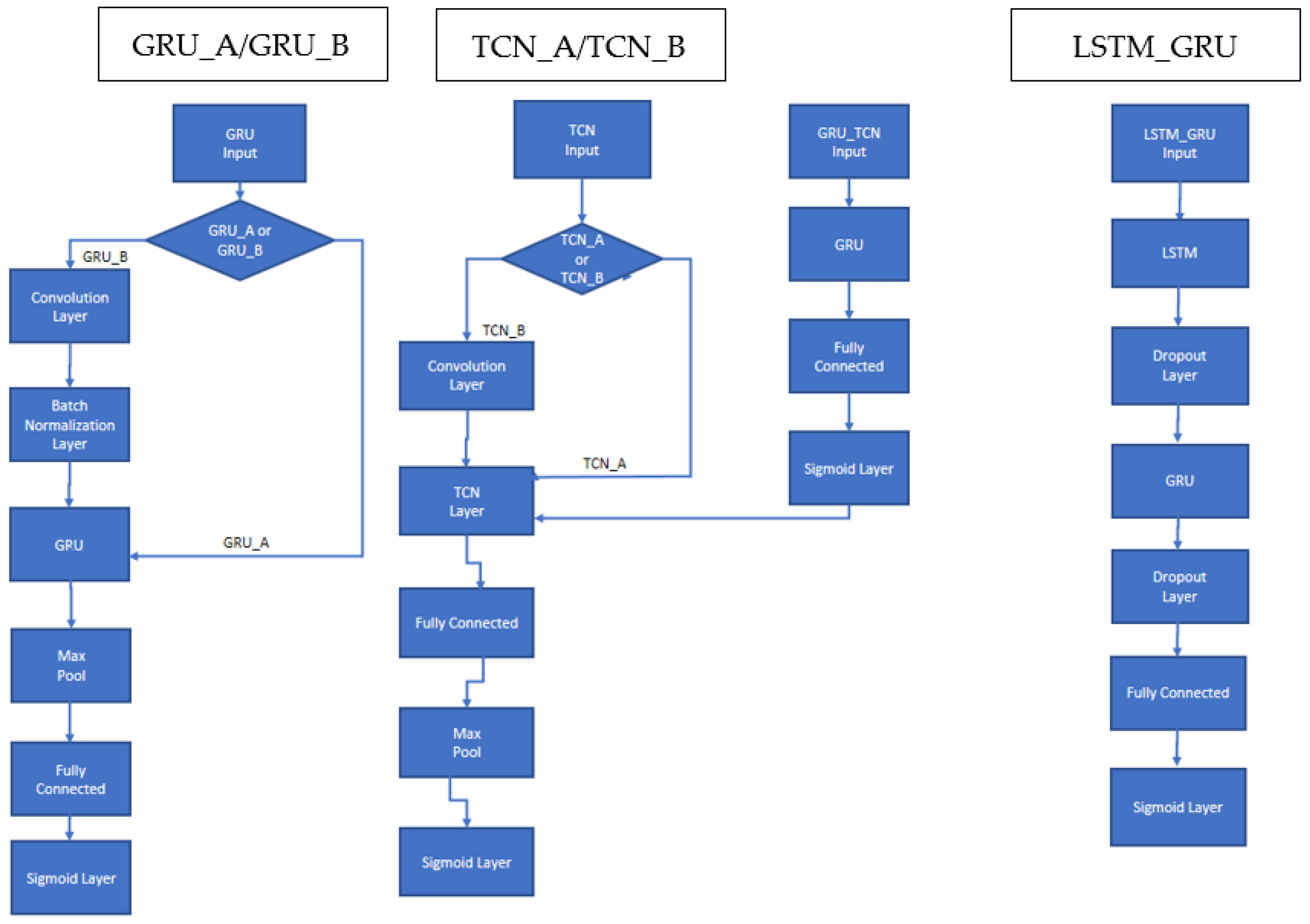
As previously indicated, the Deep Neural Network (DNN) architectures developed in this work combine LSTM, GRU, and TCN networks that have been adapted to handle multilabel classification. The general structure of each model is available in Figure 1. GRU with (N = 50) hidden units is followed by a max pooling and a fully connected layer. Multiclass classification is provided in the sigmoid output layer. TCN has a similar architecture, except that a fully connected layer is followed by a max pooling layer. These two architectures are labeled in this work GRU_A and TCN_A.

Experiments reveal that both GRU and TCN perform better in some situations when a convolutional level is placed immediately before the network itself. Convolution modifies input features with simple mathematical operations on other local features. These operations can produce better model generalization where features achieve higher special independence. When a convolutional level is attached before any TCN topologies, the network is labeled here as TCN_B.

In some GRU experiments, we add a batch-normalization layer immediately after a convolutional because batch normalization standardizes the inputs to a layer for each mini-batch, thereby stabilizing the learning process and dramatically reducing the number of training epochs required to train very deep networks. A GRU with a batch-normalization layer following a convolution is labeled GRU_B.

In addition, we investigate a sequential combination of GRU_A (without the pooling layer) followed by a TCN_A, where the sigmoid output of GRU_A becomes the input of TCN_A. This combination is labeled GRU_TCN.

The last architecture shown in Figure 1 is a network composed first of an LSTM layer with 125 hidden units followed by a dropout layer that randomly sets input elements to zero with a probability of 0.4. This is followed by a GRU layer with 100 hidden units and another dropout layer with a probability of 0.4. The end of the architecture is composed of a fully connected layer followed by a sigmoid layer.

The loss function is the binary cross entropy loss between the predicted labels (the output) and the actual labels (the target). Binary cross entropy loss computes the loss of a set of m observations by computing the following average:

$$\mathrm{CELoss}=-\frac{1}{m}{\displaystyle \sum }_{i=1}^m{\displaystyle \sum }_{j=1}^l{y}_i\left(j\right)·\log \left( {\mathit{h}}_i\left(j\right)\right)+\left(1-y_i\left(j\right)\right)·\log \left(1-{\mathit{h}}_i\left(j\right)\right)$$

(8)

where ${\mathbf{y}}_{\mathit{i}}\in {\left\{0,1\right\}}^l$and ${\mathit{h}}_{\mathit{i}}\in {\left\{0,1\right\}}^l$are the actual and predicted label vectors of each sample $\left(i\in 1\dots m\right)$, respectively.

For details on the implementation environment, see the source code at https://github.com/LorisNanni (accessed on 1 November 2022). All the code was tested and developed with MATLAB 2022a using a Titan RTX GPU.

4.2. Pre-Processing

In the main, most dataset samples require no preprocessing before being fed into our proposed networks. However, some preprocessing is needed when feature vectors are very sparse.

Two types of preprocessing were applied in our experiments:

• Feature normalization in the range [0, 1] for the dataset ATC_f for IMCC [5];
• For the datasets Liu, Arts, bibtex, enron, and health, feature transform was performed with PCA, where 99% of the variance was retained. Feature transform is only necessary for our proposed networks and not for IMCC and TB. Poor performance resulted when using the original sparse data as input to our proposed networks.

We also discovered that LSMT_GRU does not converge if a normalization step is not performed for the ATC_f dataset; it performs poorly even when the normalization step is performed. However, LSMT_GRU does converge when normalization is followed by PCA projection, where 99% of the variance is retained.

4.3. Long Short-Term Memory (LSTM)

The LSTM layer in our topologies learns long-term dependencies between the time steps in a time series and sequence data [61]. This layer performs additive interactions, which can help improve gradient flow over long sequences during training.

LTSM can be defined as follows. Let the output or hidden state be h_t, and the cell state be c_t at time step t. The first LSTM block uses the initial state of the network and the first-time step of the sequence to compute the first output and updated cell state. At time step t, the block uses the current state of the network (c_t−1, h_t−1) and the next time step of the sequence to compute the output and the updated cell state ct.

The state of the layer is the hidden state/output state and the cell state. The hidden state at time step t contains the output of the LSTM layer for this time step. The cell state contains information learned from previous time steps. At each time step, the layer adds to or removes information from the cell state. The layer controls these updates using gates.

The basic components of a LSTM are an input gate, forget gate cell candidate, and output gate: the first determines the level of cell state update, the second the level of cell state reset (forget), the third adds information to cell state, and the fourth controls the level of the cell state added to the hidden state.

Given the above and letting ${\mathrm{x}}_{\mathrm{t}}$ be the input sequence with ${\mathrm{h}}_0=0$, we can then define the input gate ${\mathrm{i}}_{\mathrm{t}}$, the forget gate ${\mathrm{f}}_{\mathrm{t}}$, the cell candidate ${\mathrm{g}}_{\mathrm{t}}$ and the output gate ${\mathrm{o}}_{\mathrm{t}}$as:

$$\begin{array}{c}{\mathrm{i}}_{\mathrm{t}}={\mathrm{o}}_{\mathrm{g}}\left({\mathrm{W}}_{\mathrm{i}}{\mathrm{x}}_{\mathrm{t}}+{\mathrm{R}}_{\mathrm{i}}{\mathrm{h}}_{\mathrm{t}-1}+{\mathrm{b}}_{\mathrm{i}}\right)\end{array}$$

(9)

$$\begin{array}{c}{\mathrm{f}}_{\mathrm{t}}={\mathrm{o}}_{\mathrm{g}}\left({\mathrm{W}}_{\mathrm{f}}{\mathrm{x}}_{\mathrm{t}}+{\mathrm{R}}_{\mathrm{f}}{\mathrm{h}}_{\mathrm{t}-1}+{\mathrm{b}}_{\mathrm{f}}\right)\end{array}$$

(10)

$$\begin{array}{c}{\mathrm{g}}_{\mathrm{t}}={\mathrm{o}}_{\mathrm{c}}\left({\mathrm{W}}_{\mathrm{g}}{\mathrm{x}}_{\mathrm{t}}+{\mathrm{R}}_{\mathrm{g}}{\mathrm{h}}_{\mathrm{t}-1}+{\mathrm{b}}_{\mathrm{g}}\right)\end{array}$$

(11)

$$\begin{array}{c}{\mathrm{o}}_{\mathrm{t}}={\mathrm{o}}_{\mathrm{g}}\left({\mathrm{W}}_{\mathrm{o}}{\mathrm{x}}_{\mathrm{t}}+{\mathrm{R}}_{\mathrm{o}}{\mathrm{h}}_{\mathrm{t}-1}+{\mathrm{b}}_{\mathrm{o}}\right)\end{array}$$

(12)

where ${\mathrm{W}}_{\mathrm{i}},{\mathrm{R}}_{\mathrm{i}},{\mathrm{b}}_{\mathrm{i}},{\mathrm{W}}_{\mathrm{f}},{\mathrm{R}}_{\mathrm{f}},{\mathrm{b}}_{\mathrm{f}},{\mathrm{W}}_{\mathrm{g}},{\mathrm{R}}_{\mathrm{g}},{\mathrm{b}}_{\mathrm{g}},{\mathrm{W}}_{\mathrm{o}},{\mathrm{R}}_{\mathrm{o}},{\mathrm{b}}_{\mathrm{o}}$ are matrices and vectors and ${\mathrm{o}}_{\mathrm{g}}$ denotes the gate activation function and σc the state activation function. The LSTM layer function, by default, uses the sigmoid function given by $\sigma \left(\mathrm{x}\right)={\left(1+{\mathrm{e}}^{-\mathrm{x}}\right)}^{-1}$ to compute the gate activation function.

We then define:

$${\mathrm{c}}_{\mathrm{t}}={\mathrm{f}}_{\mathrm{t}}\odot {\mathrm{c}}_{\mathrm{t}-1}+{\mathrm{i}}_{\mathrm{t}}\odot {\mathrm{g}}_{\mathrm{t}}$$

(13)

as the cell state, where ʘ is the Hadamard (component-wise) product.

The output vector is defined as:

$$\begin{array}{c}{\mathrm{h}}_{\mathrm{t}}={\mathrm{o}}_{\mathrm{t}} \odot {\mathsf{\sigma }}_{\mathrm{t}}\left({\mathrm{c}}_{\mathrm{t}}\right)\end{array}$$

(14)

The LSTM layer function, by default, uses the hyperbolic tangent function to compute the state activation function.

4.4. Gated Recurrent Units (GRU)

GRU [43], like LTSM, is also a recurrent neural network with a gating mechanism. GRUs can handle the gradient vanishing problem and increase the length of term dependencies from the input. GRU has a forget gate that enables the network learn which old information is relevant for understanding the new information [62]. Unlike LSTM, GRU has fewer parameters because there is no output gate, yet the performance of GRU is similar to LSTM at many tasks: speech signal modeling, polyphonic music modeling, and natural language processing [7,61]. They also perform better on small datasets [63] and work well on denoising tasks [64].

The basic components of GRU are an update gate and a reset gate. The Reset gate measures how much old information to forget. The reset gate decides which information to forget and which should be passed on to the output.

Letting $x_t$be the input sequence and $h_0=0$, the update gate vector $z_t$ and the reset gate vector $r_t$ can be defined as

$$\begin{array}{c}{z}_t=\sigma \left(W_z{x}_t+U_z{h}_{t-1}+b_z\right)\end{array}$$

(15)

$$\begin{array}{c}{r}_t=\sigma \left(W_r{x}_t+U_r{h}_{t-1}+b_r\right), \end{array}$$

(16)

where $W_z,U_z,b_z,W_r,U_r$and $b_r$ are matrices and vectors and σ is the sigmoid function.

We define

$$\begin{array}{c}{\widehat{h}}_t=\varphi \left(W_h{x}_t+U_h\left(r_t\odot h_{t-1}\right)+b_h\right)\end{array}$$

(17)

as the candidate activation vector, where ϕ is the tanh activation, and ʘ is the Hadamard (component-wise) product. The term $r_t$is the amount of past information for the candidate activation vector.

The output vector is

$$\begin{array}{c}{\widehat{h}}_t=\varphi \left(W_h{x}_t+U_h\left(r_t\odot h_{t-1}\right)+b_h\right)\end{array}$$

(18)

As can be observed, the update gate vector $z_t$ measures how much new vs. old information is combined and kept [43].

4.5. Temporal Convolutional Neural Networks (TCN)

TCNs [65] contain a hierarchy of one-dimensional convolutions stacked over time to form deep networks that perform fine-grained detection of events in sequence inputs. Subsequent layers are padded to match the size of the convolution stack, and the convolutions of each layer make use of a dilation factor that exponentially increases over the layers. In this architecture, the first layers find short-term connections in the data while the deeper layers discover longer-term dependencies based on the features extracted by previous layers. Thus, TCNs have a large receptive field that bypasses a significant limitation of most RNN architectures.

The design of TCN blocks can vary considerably. The TCN block in this work is composed of a convolution of size three with 175 different filters, followed by a ReLU and batch normalization, followed by another convolution with the same parameters, a ReLU, and batch normalization. Four of these blocks are stacked. The dilation factors of the convolutions are $2^{k-1}$, with $k$ the number of a layer. We use a fully connected layer on top, then a max pooling layer followed by the output layer. The output layer is a sigmoid layer for multiclass classification. For training, we use dropout with a probability of 0.05.

4.6. IMCC

IMMC [5] has two steps: (1) creates virtual samples to augment the training set and (2) performs multilabel training. As augmentation is what provides IMCC its performance boost, the remainder of this discussion will be on the first step.

Augmentation is performed with k-means clustering [66], along with the calculation of clustering centers. Let $X={\left[x_1,x_2\dots x_n\right]}^T\in {ℝ}^{n\times d}$ be a feature matrix and $Y={\left[y_1,y_2\dots x{y}_n\right]}^T\in {\left(-1,+1\right)}^{n\times q}$ be the label matrix, where $n$is the number of samples. If all samples are partitioned into $c$ clusters ${\mathcal{Z}}_1,{\mathcal{Z}}_2\dots {\mathcal{Z}}_c$ and $x_i$ is partitioned into cluster ${\mathcal{Z}}_j$ so that $x_i\in {\mathcal{Z}}_j$, then the average of samples should capture the semantic meaning of the cluster.

The center $z_j$ of each cluster ${\mathcal{Z}}_i$ is defined as

$$z_j=\frac{1}{\left|z_j\right|}{\displaystyle \sum }_{i=1}^{n}x·\left|\right|\left(x_i\in {\mathcal{Z}}_j\right),$$

(19)

where $\left|\right|(·)$ is an indicator function that is equal to 1 when $x_i\in {\mathcal{Z}}_j$ or to 0, otherwise [5].

A complementary training set ${\mathcal{D}}^{\prime }=\left\{z_j, t_j\right\}{}_{j=1}^c$can be generated by averaging the label vectors of all instances of ${\mathcal{Z}}_i$, thus:

$$t_j=\frac{1}{\left|z_j\right|}{\displaystyle \sum }_{i=1}^n{y}_i·\left|\right|\left(x_i\in {\mathcal{Z}}_j\right).$$

(20)

To understand more fully how the objective function deals with the original dataset $\mathcal{D}$ and the complementary dataset ${\mathcal{D}}^{\prime },$see [5]. In this study, the hyperparameters of IMCC are chosen by five-fold cross-validation on the training set.

4.7. Pooling

Pooling layers (comprised of a single max along the time dimension) are added to the end of the GRU and TCN block. In this way, the dimensionality of the processed data is reduced and only the most important information is retained, and the probability of overfitting is diminished.

4.8. Fully Connected Layer and Sigmoid Layer

The fully connected layer has l neurons, where l is the number of output labels in the given problem. This layer is fully connected with the previous layer. The activation function of this final layer is a sigmoid in the range [0…1]. These values are interpreted as the confidence relevance, or final probabilities, of each label. The output of the model is thus a multilabel classification vector, where the output of each neuron of the fully connected layer provides a score ranging from 0 to 1 for a single label in the set of labels.

4.9. Training

As noted in the introduction, training is accomplished using different Adam variants. Each of these variants is discussed below in Section 4. The learning rate is 0.01, and the gradient decay and squared gradient decay factors are 0.5 and 0.999, respectively.

In addition, gradients are cut off with a threshold equal to one using L2 norm gradient clipping. The minibatch size is set to 30, and the number of epochs in our experiments is set to 150 for GRU, LSTM_GRU, and GRU_TCN but 100 for TNC.

4.10. Ensemble Generation

Ensembles combine the outputs of more than one model. In this work, models are trained on the same problem, and their decisions are fused using the average rule. The reason for constructing ensembles is that they improve system performance and prevent overfitting. It is well known that an ensemble’s prediction and generalization increase when the diversity among the classifiers is increased.

A simple way of generating diversity in a set of neural networks is to initialize them randomly. However, applying different optimization strategies is a better way to strengthen diversity. By varying the optimization strategy, it is possible for the system to find different local minima and achieve different optima. In this work, we evaluate several Adam optimizers suitable for ensemble creation: the Adam optimizer [45], diffGrad [67] and four diffGrad variants: DGrad [68], Cos#1 [68], Exp [69], and Sto.

We generate an ensemble of 40 networks using this method: for each layer of each network, an optimization approach (DGrad, Cos#1, Exp, and Sto) is randomly selected for that layer.

5. Optimizers

5.1. Adam Optimizer

Proposed in [45], Adam calculates the adaptive learning rates for each parameter by combining momentum and adaptive gradient. The Adam update rule is based on the value of the gradient at the current step and the exponential moving averages of the gradient and its square.

Specifically, the moving averages, m_t (the first moment) and u_t (the second moment), can be defined as

$$\begin{array}{c}{m}_t={\rho }_1{m}_{t-1}+\left(1-{\rho }_1\right)g_t\end{array}$$

(21)

$$\begin{array}{c}{u}_t={\rho }_2{u}_{t-1}+\left(1-{\rho }_2\right)g_t^2\end{array}$$

(22)

where $g_t$ is the gradient at time t, the square on $g_t$ is the component-wise square, and ${\rho }_1$ and ${\rho }_2$ are hyperparameters representing the exponential decay rate for the first moment and the second moment estimates (usually set to 0.9 and 0.999), respectively, with moments initialized to 0: $m_o=u_0=0$ [45].

The values of the moving averages are very small, at least in the first few steps, due to their initialization to zero. To handle this situation, Adam is defined to correct for the bias of the moving averages:

$$\begin{array}{c}{\widehat{m}}_t=\frac{m_t}{\left(1-{\rho }_1^t\right)} \end{array}$$

(23)

$$\begin{array}{c}{\widehat{u}}_t=\frac{u_t}{\left(1-{\rho }_2^t\right)}\end{array}$$

(24)

The final update for each ${\theta }_t$ parameter of the network is

$$\begin{array}{c}{\theta }_t={\theta }_{t-1}-\lambda \frac{{\widehat{m}}_t}{\sqrt{{\widehat{u}}_t}+ϵ},\end{array}$$

(25)

where $\lambda$ is the learning rate, $ϵ$ is a small positive number to prevent division by zero (usually set to 10⁻⁸), and all operations are component-wise [45].

Though $g_t$ can have positive or negative components, $g_t^2$ can have only positive components. It is possible, therefore, that in the case where the gradient changes sign often, the value of ${\widehat{m}}_t$ could be much lower than ${\sqrt{\widehat{u}}}_t$. In this case, the step size is very small.

5.2. The DiffGrad Optimizer

The diffGrad optimizer, proposed in [67], uses the difference of the gradient to set the learning rate. Gradient changes begin to reduce during training, a behavior often indicating the presence of a global minima. The diffGrad optimizer takes advantage of this situation with an adaptive adjustment driven by the difference between the present and the immediate past values to lock parameters into a global minimum. This makes the step size larger for faster gradient changes and smaller for lower gradient changes in parameters.

For diffGrad, the update is defined as the absolute difference between two consecutive steps of the gradient:

$$\begin{array}{c}\Delta g_t=\left|g_{t-1}-g_t\right|\end{array}$$

(26)

The final update for each ${\theta }_t$ parameter of the network is Equation (28), where ${\widehat{m}}_t and {\widehat{u}}_t$ are defined as in Equations (23) and (24), but the learning rate is modulated by the Sigmoid of $\Delta g_t$ [67]:

$$\begin{array}{c}{\xi }_t=Sig\left(\Delta g_t\right)\end{array}$$

(27)

$$\begin{array}{c}{\theta }_{t+1}={\theta }_t-\lambda \cdot {\xi }_t \frac{{\widehat{m}}_t}{\sqrt{{\widehat{u}}_t}+ϵ}\end{array}$$

(28)

5.3. DiffGrad Variants

These are the variants of the diffGrad optimization method used in generating the ensembles:

• DGrad [68] is based on the moving average of the element-wise squares of the parameter gradients;
• Cos#1 [68] is a minor variant of DGrad based on the application of a cyclic learning rate [70];
• Exp is a variant of a method proposed in [69] that is based on the application of an exponential function;
• Sto is a stochastic approach that stalls the optimizer on flat surfaces or small wells.

The proposed approaches have different methods for defining ${\xi }_t$, followed by the application of Equation (28) to calculate the final update for ${\theta }_t$.

The rationale for all these variants is to avoid optimizer stalling on flat surfaces due to the low value of $\Delta g_t$.

DGrad [68] differs from diffGrad by defining the absolute difference between two consecutive steps of the gradient as

$$\mathsf{\Delta }a{g}_t=|g_t-av{g}_t|,$$

(29)

where $av{g}_t$contains the moving average of the element-wise squares of the parameter gradients; we then normalize $\Delta a{g}_t$ by its maximum as

$$\begin{array}{c}\Delta \widehat{a{g}_t}=\left(\frac{\Delta a{g}_t}{\max \left(\Delta a{g}_t\right)}\right)\end{array}$$

(30)

With DGrad, ${\xi }_t$ is defined as the Sigmoid of $4\cdot \Delta \widehat{a{g}_t}$. The rationale for multiplying by four is to exploit the range of the output of the sigmoid function [68]:

$$\begin{array}{c}{\xi }_t=Sig\left(4\cdot \Delta \widehat{a{g}_t}\right)\end{array}$$

(31)

Cos#1 [68] is a variant of DGrad with a cyclic learning rate. The idea is to improve classification accuracy without tuning and with fewer iterations [17]. In this work, the cos() periodic function is selected to define a range of variation in the learning rate:

$$\begin{array}{c}l{r}_t=\left(2-\left|\cos \left(\frac{\pi \cdot t}{steps}\right)\right|e^{-0.01\cdot \left(mod\left(t,steps\right)+1\right)}\right),\end{array}$$

(32)

where mod() denotes the function modulo and where steps = 30 is the period [68]. The plot of $l{r}_t$ for t in the range 1:2 × steps is reported in Figure 2.

With Cos#1, $l{r}_t$ is used as a multiplier of $\Delta \widehat{a{g}_t}$ in the definition of ${\xi }_t$ (Equation (31)):

$$\begin{array}{c}{\xi }_t=Sig\left(4\cdot l{r}_t\cdot \Delta \widehat{a{g}_t}\right)\end{array}$$

(33)

Exp [69] performs the element-wise operations of product and exponential. Exp is designed to reduce the impact of large variations in the gradient and help the function converge for small values. The function in Equation (34) decays slower than the negative exponential for larger values. It also provides less focus on gradient variations that tend to zero. A larger area of greater gain is thus produced [69]:

$$\begin{array}{c}l{r}_t= \Delta a{g}_t·e^{\left(-k·\Delta a{g}_t\right)},\end{array}$$

(34)

with k set to 2 in our experiments.

The final learning rate (${\xi }_t$) is the normalized result multiplied by a correction factor (1.5), which moves the mean towards the unit as illustrated in Figure 3:

$$\begin{array}{c}{\xi }_t=1.5\frac{l{r}_t}{\max \left(l{r}_t\right)}\end{array}$$

(35)

Sto (short for Stochastic), proposed here, adds noise to the learning rate to reduce the tendency to stall on flat surfaces or small wells. The noise is independent of the gradient direction.

Let $\mathcal{X}$ be a matrix of independent uniform random variables in range [0,1] and J an all-ones matrix:

$$\mathcal{X}=\left[\begin{array}{ccc}{X}_{1,1}& \cdots & X_{1,n}\\ ⋮& \ddots & ⋮\\ X_{m,1}& \cdots & X_{m,n}\end{array}\right]\mathrm{and}J=\left[\begin{array}{ccc}1& \cdots & 1\\ ⋮& \ddots & ⋮\\ 1& \cdots & 1\end{array}\right],$$

where $X_{i,j}~\mathcal{U}\left(0,1\right)$ are random variables with a uniform density function. The learning rate is defined as

$$\begin{array}{c}l{r}_t=\Delta a{g}_t·e^{\left(-4·\Delta a{g}_t\right)}·\left(\mathcal{X}+0.5·J\right)\end{array}$$

(36)

$$\begin{array}{c}{\xi }_t=1.5\frac{l{r}_t}{\max \left(l{r}_t\right)} \end{array}$$

(37)

In Equation (36), matrix J shifts the range of $X$ by 0.5 to move the mean across 1.

6. Experimental Results

The goal of the first experiment was to build and evaluate the performance of the different variants of the base models combined with all the components detailed in Section 4 and Section 5. All ensembles were fused by the average rule. In

Table 3. Summary of tested ensembles.

Name	Hidden Units	#Classifiers	#Epoch	Optimizer
Adam_sa	50	1	50	Adam
Adam_10s	50	10	50	Adam
Adam_10	50	10	150	Adam
DG_10	50	10	150	DGrad
Cos_10	50	10	150	Cos
Exp_10	50	10	150	Exp
Sto_10	50	10	150	Sto
DG_Cos = DG_10 + Cos_10	50	20	150	DGrad, Cos
DG_Cos_Exp = DG_10 + Cos_10 + Exp_10	50	30	150	DGrad, Cos, Exp
DG_Cos_Exp_Sto = DG_10 + Cos_10 + Exp_10 + Sto_10	50	40	150	DGrad, Cos, Exp, Sto
StoGRU	50	40	150	DGrad, Cos, Exp, Sto
StoGRU_B	50	40	150	DGrad, Cos, Exp, Sto
StoTCN	---	40	100	DGrad, Cos, Exp, Sto
StoTCN_B	---	40	100	DGrad, Cos, Exp, Sto
StoGRU_TCN	50 (GRU)	40	150	DGrad, Cos, Exp, Sto
StoLSTM_GRU	125 (LSTM layer) 100 (GRU layer)	40	150	DGrad, Cos, Exp, Sto
ENNbase = StoTCN+StoGRU	50 (GRU)	80	100 (TCN)/150 (GRU)	DGrad, Cos, Exp, Sto
ENN = StoTCN + StoGRU + StoTCN_B + StoGRU_B + StoGRU_TCN	50 (GRU, GRU_B & GRU_TCN)	200	100 (TCN & TCN_B)/150 (GRU, GRU_B & GRU_TCN)	DGrad, Cos, Exp, Sto
ENNlarge = StoTCN + StoGRU + StoTCN_B + StoGRU_B + StoGRU_TCN + StoLSTM_GRU	50 (GRU, GRU_B & GRU_TCN) 100/125 (LSTM_GRU)	240	100 (TCN & TCN_B)/150 (GRU, GRU_B, LSTM_GRU & GRU_TCN)	DGrad, Cos, Exp, Sto

, we provide a summary of each of these ensembles: the number of classifiers and hidden units, the number of training epochs, and the loss function. Given a base standalone GRU_A with 50 hidden units trained by Adam for 50 epochs (labeled Adam_sa), we generated different ensembles by incrementally increasing complexity. We do this by combining ten Adam_sa (Adam_10s), increasing the number of epochs to 150 (Adam_10), selecting differnt optimizers (DG_10, Cos_10, Exp_10, Sto_10), and fusing the best results in the following ways:

• DG_Cos is the fusion of DG_10 + Cos_10;
• DG_Cos_Exp is the fusion of DG_10 + Cos_10 + Exp_10;
• DG_Cos_Exp_Sto is the fusion of DG_10 + Cos_10 + Exp_10 + Sto_10;
• StoGRU is an ensemble composed of 40 GRU_A, combined by average rule, each coupled with the stocastic approach explained in Section 4.10;
• StoGRU_B as StoGRU but based on GRU_B;
• StoTCN is an ensemble of 40 TCN_A, combined by average rule, each coupled with the stochastic approach explained in Section 4.10;
• StoTCN_B as StoTCN but based on TCN_B;
• StoGRU_TCN is an ensemble of 40 GRU_TCN each coupled with the stochastic approach explained in Section 4.10;
• StoLSTM_GRU is an ensemble of 40 LSTM_GRU each coupled with the stochastic approach explained in Section 4.10;
• ENNbase is the fusion by average rule of StoGRU and StoTCN;
• ENN is the fusion by average rule of StoGRU, StoTCN, StoGRU_B, StoTCN_B and StoGRU_TCN;
• ENNlarge is the fusion by average rule of StoGRU, StoTCN, StoGRU_B, StoTCN_B, StoGRU_TCN and StoLSTM_GRU.

An ablation study for assessing the performance improvement that each module of our ensemble achieved is reported in

Table 4. Ablation study showing that StoGRU is the best method among the approaches based on GRU_A (other approaches produced similar results).

Method	Comparison
Adam_10s	Outperforms Adam_sa with a p-value of 0.0156
Adam_10	Outperforms Adam_sa with a p-value of 0.0172 Same performance of Adam_10s
DG_10	Outperforms Adam_10 with a p-value of 0.0064
Cos_10	Outperforms Adam_10 with a p-value of 0.0137
Exp_10	Outperforms Adam_10 with a p-value of 0.0016
Sto_10	Outperforms Adam_10 with a p-value of 0.1014
DG_Cos_Exp_Sto	Outperforms Exp_10 (the best of the approaches reported above in this table) with a p-value of 0.0134
StoGRU	Outperforms DG_Cos_Exp_Sto with a p-value of 0.0922

. Only tests on GRU_A is reported here. The other topologies tested in this work produced similar conclusions. In Table 4, we compare approaches using Wilcoxon signed rank test.

Table 5. Average precision of the ensembles and state of the art on the twelve benchmarks (boldface values indicate the best performance within each group of similar approaches). Bold highlights superior performance.

Average Precision	Cal500	Image	Scene	Yeast	Arts	ATC	ATC_f	Liu	mAn	Bibtex	Enron	Health	Ave
IMCC	0.502	0.836	0.904	0.773	0.619	0.866	0.922	0.523	0.978	0.623	0.714	0.781	0.753
TB	0.489	0.844	0.873	0.778	0.625	0.882	0.897	0.518	0.983	0.572	0.701	0.753	0.743
StoGRU	0.498	0.851	0.911	0.740	0.561	0.872	0.872	0.485	0.979	0.403	0.680	0.739	0.715
StoGRU_B	0.490	0.861	0.908	0.741	0.555	0.877	0.848	0.485	0.978	0.400	0.688	0.724	0.712
StoTCN	0.498	0.847	0.913	0.764	0.506	0.882	0.900	0.498	0.977	0.406	0.669	0.710	0.714
StoTCN_B	0.497	0.855	0.917	0.765	0.541	0.883	0.903	0.505	0.976	0.404	0.666	0.732	0.720
StoGRU_TCN	0.491	0.852	0.916	0.752	0.592	0.890	0.913	0.510	0.977	0.354	0.674	0.764	0.724
StoLSTM_GRU	0.493	0.839	0.901	0.771	0.633	0.888	0.912	0.541	0.978	0.618	0.702	0.790	0.756
ENNbase	0.502	0.855	0.922	0.756	0.552	0.888	0.916	0.497	0.979	0.417	0.687	0.735	0.726
ENN	0.499	0.859	0.924	0.762	0.582	0.893	0.916	0.505	0.979	0.424	0.689	0.749	0.732
ENNlarge	0.498	0.860	0.923	0.776	0.628	0.892	0.926	0.520	0.979	0.534	0.708	0.780	0.752
ENNlarge + IMCC	0.502	0.853	0.920	0.784	0.633	0.883	0.926	0.526	0.979	0.627	0.717	0.790	0.762
ENNlarge + 3 × IMCC	0.503	0.847	0.913	0.778	0.628	0.875	0.925	0.526	0.979	0.626	0.718	0.787	0.759
ENNlarge + IMCC + TB	0.500	0.856	0.913	0.784	0.641	0.889	0.927	0.526	0.982	0.622	0.718	0.788	0.762
ENNlarge + 3 × IMCC + TB	0.502	0.850	0.910	0.783	0.637	0.880	0.926	0.527	0.981	0.627	0.717	0.787	0.761
StoLSTM_GRU + IMCC + TB	0.500	0.851	0.898	0.786	0.641	0.883	0.920	0.538	0.983	0.635	0.727	0.800	0.764

shows the performance of the ensembles in Table 3 in terms of average precision. Moreover, we report the performance of IMCC [5] and TB. For both IMCC and TB, the hyperparameters were chosen by a five-fold cross-validation on the training set. Also reported in this table are the different fusions among ENNlarge, IMCC, and TB:

• ENNlarge + w × IMCC is the sum rule between ENNlarge and IMCC; before fusion, the scores of ENNlarge (notice that the ensemble ENNlarge is obtained by average rule) were normalized since it has a different range of values compared to IMCC. Normalization was performed as $ENNlarge=\left(ENNlarge-0.5\right)\times 2$, the classification threshold of the the ensemble is simply set to zero. The scores of IMCC were weighted by a factor of w.
• ENNlarge + w × IMCC + TB is the same as the previous fusion, but TB is included in the ensemble. Before fusion, the scores of TB were normalized since it has a different range of values compared to IMCC. Normalization was performed as $TB=\left(TB-0.5\right)\times 2$.
• StoLSTM_GRU + IMCC + TB is the sum rule among StoLSTM_GRU, IMCC, and TB. StoLSTM_GRU and TB are normalized before the fusion as $StoLST{M}_{G}RU=\left(StoLST{M}_{G}RU-0.5\right)\times 2;TB=\left(TB-0.5\right)\times 2$.

IMCC and TB do not use PCA when sparse datasets are tested, as noted in Section 4.2.

These are some of the conclusions that can be drawn from examining Table 5:

• GRU/TCN-based methods work poorly on very sparse datasets (i.e., on Arts, Liu, bibtex, enron, and health);
• StoGRU_TCN outperforms the other ensembles based on GRU/TCN; StoGRU and StoTCN perform similarly;
• StoLSTM_GRU works very well on sparse datasets. On datasets that are not sparse, the performance is similar to that obtained by the other methods based on GRU/TCN. StoLSTM_GRU average performance is higher than that obtained by IMCC;
• ENNlarge outperforms each method from which it was built;
• ENNlarge + 3 × IMCC+TB outperforms ENNlarge+3×IMCC with a p-value 0.09;
• StoLSTM_GRU + IMCC + TB is the best choice for sparse datasets;
• ENNlarge + 3 × IMCC + TB tops or equals IMCC in all the datasets (note that ENN+IMCC+TB and StoLSTM_GRU+IMCC+TB have performance equal to or lower than IMCC in some datasets). ENNlarge + 3 × IMCC + TB is our suggested approach.
• In the following tests, we simplify the names of our best ensembles to reduce clutter:
• Ens refers to ENNlarge + 3 × IMCC+TB;
• EnsSparse refers to StoLSTM_GRU + IMCC + TB.

In

Table 6. Comparison of IMCC and our proposed ensemble ENS using five performance indicators. Bold highlights superior performance.

	One Error ↓	Hamming Loss ↓	Ranking Loss ↓	Coverage ↓	Avg Precision ↑
Cal500-IMCC	0.150	0.134	0.182	0.736	0.502
Cal500-Ens	0.150	0.134	0.179	0.729	0.502
Image-IMCC	0.237	0.150	0.138	0.173	0.836
Image-Ens	0.225	0.147	0.127	0.159	0.850
scene-IMCC	0.164	0.070	0.053	0.062	0.904
scene-Ens	0.151	0.067	0.047	0.057	0.910
Yest-IMCC	0.220	0.185	0.165	0.448	0.773
Yest-Ens	0.211	0.178	0.155	0.433	0.783
Arts-IMCC	0.438	0.054	0.164	0.242	0.619
Arts-Ens	0.431	0.053	0.144	0.219	0.637
Bibtex-IMCC	0.336	0.012	0.079	0.158	0.623
Bibtex-Ens	0.338	0.012	0.072	0.143	0.627
Enron-IMCC	0.226	0.044	0.072	0.211	0.714
Enron-Ens	0.226	0.044	0.069	0.204	0.717
Health-IMCC	0.266	0.035	0.052	0.107	0.781
Health-Ens	0.262	0.035	0.046	0.097	0.787

, we compare IMCC and Ens using more performance indicators. Our ensemble Ens outperforms IMCC.

In

Table 7. Performance comparison of Ens and IMCC on the mAn data set. Bold highlights superior performance.

mAn	Aiming	Coverage	Accuracy	Absolute True	Absolute False
[2]	88.31	85.06	84.34	78.78	0.07
[4]	96.21	97.77	95.46	92.26	0.00
IMCC	92.80	92.02	88.83	80.76	1.43
Ens	93.84	93.06	90.24	83.64	1.20

, we compare Ens with state of the art on the mAn dataset using the performance measures covered in the literature for this dataset, viz., coverage, accuracy, absolute true, and absolute false.

Ens outperforms IMCC on mAn on these five measures; however, Ens does not achieve top performance. A recent ad hoc method [4] does better on this dataset than does Ens.

In

Table 8. Comparisons with results reported in a recent survey [71] using average precision as the performance indicator. Bold highlights superior performance.

	EPS	CDE	MLkNN	MLARM	BR	DEEP1	PCT	HOMER	AdaBoost.MH	BPNN	RAkEL	CLR	RFPCT	PSt	TREMLC	RFDTBR	MBR	CDN	ECCJ48	EBRJ48	DEEP4	RSLP	CLEMS	Ens
bibtex	0.466	0.414	0.161	0.423	0.350	0.335	0.016	0.316	0.472	0.434	0.081	0.463	0.515	0.538	0.483	0.559	0.265	0.231	0.492	0.546	0.258	0.491	0.183	0.627
Cal500	0.440	0.411	0.441	0.352	0.236	0.489	0.497	0.288	0.475	0.508	0.271	0.355	0.520	0.485	0.497	0.500	0.381	0.292	0.427	0.458	0.329	0.490	0.446	0.502
enron	0.622	0.580	0.517	0.529	0.512	0.624	0.531	0.388	0.627	0.642	0.447	0.623	0.683	0.629	0.675	0.686	0.498	0.485	0.623	0.675	0.537	0.548	0.538	0.717
scene	0.789	0.812	0.785	0.715	0.790	0.686	0.745	0.753	0.880	0.855	0.851	0.889	0.868	0.887	0.856	0.874	0.711	0.501	0.813	0.856	0.810	0.797	0.850	0.910
yeast	0.745	0.718	0.704	0.598	0.663	0.701	0.732	0.693	0.711	0.761	0.693	0.710	0.762	0.766	0.760	0.763	0.576	0.437	0.719	0.740	0.709	0.748	0.715	0.787

, we show the performance reported in a recent survey [71] of many multilabel methods (the meaning of the acronyms and sources are noted in [71] and not included here as the intention of this table to demonstrate the superiority of Ens compared to the score reported in the survey). The last column reports the performance of our proposed ensemble. As can be observed, it obtains the average best performance.

Finally, in

Table 9. Other comparisons with the literature using average precision. Bold highlights superior performance.

Average Precision	Cal500	Image	Scene	Yeast	Arts	ATC	ATC_f	Liu	mAn	Bibtex	Enron	Health
Ens	0.503	0.849	0.912	0.780	0.632	0.878	0.926	0.527	0.981	0.626	0.717	0.788
EnsSparse	0.500	0.851	0.898	0.786	0.641	0.883	0.920	0.538	0.983	0.635	0.727	0.800
FastAi [32]	0.425	0.824	0.899	0.718	0.588	0.860	0.908	0.414	0.976	---	---	---
IMCC	0.502	0.836	0.904	0.773	0.619	0.866	0.922	0.523	0.978	0.623	0.714	0.781
hML	0.453	0.810	0.885	0.792	0.538	0.831	0.854	0.433	0.965	---	---	---
ECC [5]	0.491	0.797	0.857	0.756	0.617	---	---	---	---	0.617	0.657	0.719
MAHR [5]	0.441	0.801	0.861	0.745	0.524	---	---	---	---	0.524	0.641	0.715
LLSF [5]	0.501	0.789	0.847	0.617	0.627	---	---	---	---	0.627	0.703	0.780
JFSC [5]	0.501	0.789	0.836	0.762	0.597	---	---	---	---	0.597	0.643	0.751
LIFT [5]	0.496	0.789	0.859	0.766	0.627	---	---	---	---	0.627	0.684	0.708
[15]	---	---	---	---	---	---	---	0.513	---	---	---	---
[72]	---	---	---	---	---	---	---	0.261	---	---	---	---
hMuLab [18]	---	---	---	0.778	---	---	---	---	---	---	---	---
MlKnn [18]	---	---	---	0.766	---	---	---	---	---	---	---	---
RaKel [18]	---	---	---	0.715	---	---	---	---	---	---	---	---
ClassifierChain [18]	---	---	---	0.624	---	---	---	---	---	---	---	---
IBLR [18]	---	---	---	0.768	---	---	---	---	---	---	---	---
MLDF [73]	0.512	0.842	0.891	0.770	---	---	---	---	---	---	0.742	---
RF_PCT [73]	0.512	0.829	0.873	0.758	---	---	---	---	---	---	0.729	---
DBPNN [73]	0.495	0.672	0.563	0.738	---	---	---	---	---	---	0.679	---
MLFE [73]	0.488	0.817	0.882	0.759	---	---	---	---	---	---	0.656	---
ECC [73]	0.482	0.739	0.853	0.752	---	---	---	---	---	---	0.646	---
RAKEL [73]	0.353	0.788	0.843	0.720	---	---	---	---	---	---	0.596	---
[14]	---	---	---	0.758	---	---	---	---	---	---	---	---
[74]	0.484	---	---	0.740	---	---	---	---	---	---	---	---
[75]	---	---	---	0.775	0.636	---	---	---	---	---	---	---
Wrap [76]	0.520	---	0.832	0.761	---	---	---	---	---	0.578	0.710	---
Wrapk [76]	0.518	---	0.892	0.781	---	---	---	---	---	0.571	0.720	---

, our best ensembles, Ens and EnsSparse, are compared with the literature across all twelve benchmarks using average precision as the performance indicator. Ens and EnsSparse obtain state-of-the-art performance using this measure on several of the multilabel benchmarks.

7. Conclusions

The system proposed in this work for multilabel classification is composed of ensembles of gated recurrent units (GRU), temporal convolutional neural networks (TCN) and long short-term memory networks (LSTM) trained with several variants of Adam optimization. This approach combines Incorporating Multiple Clustering Centers (IMCC) to produce an even better multilabel classification system. Many ensembles are tested across a set of twelve multilabel benchmarks representing many different applications. Experimental results show that the best ensemble constructed using our novel approach obtains state-of-the-art performance.

Future studies will focus on combining our proposed method with other topologies for extracting features. Moreover, more sparse datasets will be used to evaluate the performance of the proposed ensemble for further validation of the conclusions drawn in this work.

Another area of research will be to investigate deep ensembling techniques for multilabel classification that utilizes edge intelligence. Accelerated by the success of AI and IoT technologies, there is an urgent need to push the AI frontiers to the network edge to fully unleash the potential of big data. Edge Computing is a promising concept to support computation-intensive AI applications on edge devices [77]. Edge Intelligence or Edge AI is a combination of AI and Edge Computing; it enables the deployment of machine learning algorithms to the edge devices where the data is generated. One of the main problems in edge intelligence is how to apply ensemble systems usually developed for high performance servers. A possible solution is to adopt and develop distillation approaches. For example, in [78], the authors propose a framework for learning compact deep learning models.

References

1. Galindo, E.G.; Ventura, S. Multi label learning: A review of the state of the art and ongoing research. Wiley Interdiscip. Rev. Data Min. Knowl. Discov. 2014, 4, 411–444. [Google Scholar] [CrossRef]
2. Cheng, X.; Lin, W.-Z.; Xiao, X.; Chou, K.-C. pLoc_bal-mAnimal: Predict subcellular localization of animal proteins by balancing training dataset and PseAAC. Bioinformatics 2018, 35, 398–406. [Google Scholar] [CrossRef] [PubMed]
3. Chen, L.; Li, Z.; Zeng, T.; Zhang, Y.-H.; Li, H.; Huang, T.; Cai, Y.-D. Predicting gene phenotype by multi-label multi-class model based on essential functional features. Mol. Genet. Genom. MGG 2021, 296, 905–918. [Google Scholar] [CrossRef] [PubMed]
4. Shao, Y.; Chou, K. pLoc_Deep-mAnimal: A Novel Deep CNN-BLSTM Network to Predict Subcellular Localization of Animal Proteins. Nat. Sci. 2020, 12, 281–291. [Google Scholar] [CrossRef]
5. Shu, S.; Lv, F.; Feng, L.; Huang, J.; He, S.; He, J.; Li, L. Incorporating Multiple Cluster Centers for Multi-Label Learning. arXiv 2020, arXiv:2004.08113. [Google Scholar] [CrossRef]
6. Ibrahim, M.; Khan, M.U.G.; Mehmood, F.; Asim, M.; Mahmood, W. GHS-NET a generic hybridized shallow neural network for multi-label biomedical text classification. J. Biomed. Inform. 2021, 116, 103699. [Google Scholar] [CrossRef]
7. Ravanelli, M.; Brakel, P.; Omologo, M.; Bengio, Y. Light Gated Recurrent Units for Speech Recognition. IEEE Trans. Emerg. Top. Comput. Intell. 2018, 2, 92–102. [Google Scholar] [CrossRef] [Green Version]
8. Kim, Y.; Kim, J. Human-Like Emotion Recognition: Multi-Label Learning from Noisy Labeled Audio-Visual Expressive Speech. In Proceedings of the 2018 IEEE International Conference on Acoustics, Speech and Signal Processing (ICASSP), Calgary, AB, Canada, 15–20 April 2018. [Google Scholar]
9. Messaoud, M.B.; Jenhani, I.; Jemaa, N.B.; Mkaouer, M.W. A Multi-label Active Learning Approach for Mobile App User Review Classification. In Proceedings of the KSEM, Athens, Greece, 28–30 August 2019. [Google Scholar]
10. Singh, J.P.; Nongmeikapam, K. Negative Comments Multi-Label Classification. In Proceedings of the 2020 International Conference on Computational Performance Evaluation (ComPE), Shillong, India, 2–4 July 2020; pp. 379–385. [Google Scholar] [CrossRef]
11. Boutell, M.; Luo, J.; Shen, X.; Brown, C.M. Learning multi-label scene classification. Pattern Recognit. 2004, 37, 1757–1771. [Google Scholar] [CrossRef] [Green Version]
12. Tsoumakas, G.; Katakis, I.; Vlahavas, I. Mining Multi-label Data. In Data Mining and Knowledge Discovery Handbook; Springer: New York, NY, USA, 2020; pp. 667–685. [Google Scholar]
13. Read, J.; Pfahringer, B.; Holmes, G.; Frank, E. Classifier chains for multi-label classification. Mach Learn. 2011, 85, 333–359. [Google Scholar] [CrossRef]
14. Qian, W.; Xiong, C.; Wang, Y. A ranking-based feature selection for multi-label classification with fuzzy relative discernibility. Appl. Soft Comput. 2021, 102, 106995. [Google Scholar] [CrossRef]
15. Zhang, W.; Liu, F.; Luo, L.; Zhang, J. Predicting drug side effects by multi-label learning and ensemble learning. BMC Bioinform. 2015, 16, 365. [Google Scholar] [CrossRef] [PubMed] [Green Version]
16. Huang, J.; Li, G.; Huang, Q.; Wu, X. Joint Feature Selection and Classification for Multilabel Learning. IEEE Trans. Cybern. 2018, 48, 876–889. [Google Scholar] [CrossRef] [PubMed]
17. Huang, J.; Li, G.; Huang, Q.; Wu, X. Learning Label-Specific Features and Class-Dependent Labels for Multi-Label Classification. IEEE Trans. Knowl. Data Eng. 2016, 28, 3309–3323. [Google Scholar] [CrossRef]
18. Wang, P.; Ge, R.; Xiao, X.; Zhou, M.; Zhou, F. hMuLab: A Biomedical Hybrid MUlti-LABel Classifier Based on Multiple Linear Regression. IEEE/ACM Trans. Comput. Biol. Bioinform. 2017, 14, 1173–1180. [Google Scholar] [CrossRef]
19. Tsoumakas, G.; Katakis, I.; Vlahavas, I. Random k-Labelsets for Multilabel Classification. IEEE Trans. Knowl. Data Eng. 2011, 23, 1079–1089. [Google Scholar] [CrossRef]
20. Yang, Y.; Jiang, J. Adaptive Bi-Weighting Toward Automatic Initialization and Model Selection for HMM-Based Hybrid Meta-Clustering Ensembles. IEEE Trans. Cybern. 2019, 49, 1657–1668. [Google Scholar] [CrossRef]
21. Moyano, J.M.; Galindo, E.G.; Cios, K.; Ventura, S. Review of ensembles of multi-label classifiers: Models, experimental study and prospects. Inf. Fusion 2018, 44, 33–45. [Google Scholar] [CrossRef]
22. Xia, Y.; Chen, K.; Yang, Y. Multi-label classification with weighted classifier selection and stacked ensemble. Inf. Sci. 2021, 557, 421–442. [Google Scholar] [CrossRef]
23. Moyano, J.M.; Galindo, E.G.; Cios, K.; Ventura, S. An evolutionary approach to build ensembles of multi-label classifiers. Inf. Fusion 2019, 50, 168–180. [Google Scholar] [CrossRef]
24. Wang, R.; Kwong, S.; Wang, X.; Jia, Y. Active k-labelsets ensemble for multi-label classification. Pattern Recognit. 2021, 109, 107583. [Google Scholar] [CrossRef]
25. DeepDetect. DeepDetect. Available online: https://www.deepdetect.com/ (accessed on 1 January 2021).
26. Simonyan, K.; Zisserman, A. Very Deep Convolutional Networks for Large-Scale Image Recognition; Cornell University: Ithaca, NY, USA, 2014. [Google Scholar]
27. Szegedy, C.; Vanhoucke, V.; Ioffe, S.; Shlens, J.; Wojna, Z. Rethinking the inception architecture for computer vision. In Proceedings of the IEEE Conference on Computer Vision and Pattern Recognition, Las Vegas, NV, USA, 27–30 June 2016; pp. 2818–2826. [Google Scholar]
28. Szegedy, C.; Ioffe, S.; Vanhoucke, V.; Alemi, A. Inception-v4, Inception-Resnet and the Impact of Residual Connections on Learning; Cornell University: Ithaca, NY, USA, 2016; pp. 1–12. Available online: https://arxiv.org/pdf/1602.07261.pdf (accessed on 1 January 2021).
29. He, K.; Zhang, X.; Ren, S.; Sun, J. Deep Residual Learning for Image Recognition. In Proceedings of the 2016 IEEE Conference on Computer Vision and Pattern Recognition (CVPR), Las Vegas, NV, USA, 27–30 June 2016; pp. 770–778. [Google Scholar]
30. Sandler, M.; Howard, A.; Zhu, M.; Zhmoginov, A.; Chen, L. MobileNetV2: Inverted Residuals and Linear Bottlenecks. In Proceedings of the 2018 IEEE/CVF Conference on Computer Vision and Pattern Recognition, Salt Lake City, UT, USA, 18–23 June 2018; pp. 4510–4520. [Google Scholar]
31. Redmon, J.; Farhadi, A. YOLOv3: An Incremental Improvement. arXiv 2018, arXiv:1804.02767. [Google Scholar]
32. Howard, J.; Gugger, S. Fastai: A Layered API for Deep Learning. Information 2020, 11, 108. [Google Scholar] [CrossRef] [Green Version]
33. Imagga. Imagga Website. Available online: https://imagga.com/solutions/auto-tagging (accessed on 1 January 2021).
34. Wolfram. Wolfram Alpha: Image Identification Project. Available online: https://www.imageidentify.com/ (accessed on 1 January 2020).
35. Clarifai. Clarifai Website. Available online: https://www.clarifai.com/ (accessed on 1 January 2021).
36. Microsoft. Computer-Vision API Website. Available online: https://www.microsoft.com/cognitive-services/en-us/computer-vision-api (accessed on 1 January 2021).
37. IBM. Visual Recognition. Available online: https://www.ibm.com/watson/services/visual-recognition/ (accessed on 1 January 2020).
38. Google. Google Cloud Vision. Available online: https://cloud.google.com/vision/ (accessed on 1 January 2021).
39. Kubany, A.; Ishay, S.B.; Ohayon, R.-s.; Shmilovici, A.; Rokach, L.; Doitshman, T. Comparison of state-of-the-art deep learning APIs for image multi-label classification using semantic metrics. Expert Syst. Appl. 2020, 161, 113656. [Google Scholar] [CrossRef]
40. Ho, T.K. The random subspace method for constructing decision forests. IEEE Trans. Pattern Anal. Mach. Intell. 1998, 20, 832–844. [Google Scholar]
41. Li, D.; Wu, H.; Zhao, J.; Tao, Y.; Fu, J. Automatic Classification System of Arrhythmias Using 12-Lead ECGs with a Deep Neural Network Based on an Attention Mechanism. Symmetry 2020, 12, 1827. [Google Scholar] [CrossRef]
42. Hochreiter, S.; Schmidhuber, J. Long short-term memory. Neural Comput. 1997, 9, 1735–1780. [Google Scholar] [CrossRef] [PubMed]
43. Cho, K.; Merrienboer, B.V.; Gülçehre, Ç.; Bahdanau, D.; Bougares, F.; Schwenk, H.; Bengio, Y. Learning Phrase Representations using RNN Encoder Decoder for Statistical Machine Translation. In Proceedings of the EMNLP, Varna, Bulgaria, 25–29 October 2014; pp. 25–32. [Google Scholar]
44. Lea, C.S.; Flynn, M.D.; Vidal, R.; Reiter, A.; Hager, G. Temporal Convolutional Networks for Action Segmentation and Detection. In Proceedings of the 2017 IEEE Conference on Computer Vision and Pattern Recognition (CVPR), Honolulu, HI, USA, 21–26 July 2017; pp. 1003–1012. [Google Scholar]
45. Kingma, D.P.; Ba, J. Adam: A Method for Stochastic Optimization. arXiv 2015, arXiv:1412.6980. [Google Scholar]
46. Nanni, L.; Lumini, A.; Manfe, A.; Brahnam, S.; Venturin, G. Gated recurrent units and temporal convolutional network for multilabel classification. arXiv 2021, arXiv:2110.04414. [Google Scholar]
47. Zhang, M.-L.; Zhou, Z.-H. Multilabel Neural Networks with Applications to Functional Genomics and Text Categorization. IEEE Trans. Knowl. Data Eng. 2006, 18, 1338–1351. [Google Scholar] [CrossRef] [Green Version]
48. Stivaktakis, R.; Tsagkatakis, G.; Tsakalides, P. Deep Learning for Multilabel Land Cover Scene Categorization Using Data Augmentation. IEEE Geosci. Remote Sens. Lett. 2019, 16, 1031–1035. [Google Scholar] [CrossRef]
49. Zhu, H.; Cheng, C.; Yin, H.; Li, X.; Zuo, P.; Ding, J.; Lin, F.; Wang, J.; Zhou, B.; Li, Y.; et al. Automatic multilabel electrocardiogram diagnosis of heart rhythm or conduction abnormalities with deep learning: A cohort study. Lancet. Digit. Health 2020, 2, e348–e357. [Google Scholar] [CrossRef] [PubMed]
50. Navamajiti, N.; Saethang, T.; Wichadakul, D. McBel-Plnc: A Deep Learning Model for Multiclass Multilabel Classification of Protein-lncRNA Interactions. In Proceedings of the 2019 6th International Conference on Biomedical and Bioinformatics Engineering (ICBBE’19), Shanghai, China, 13–15 November 2019. [Google Scholar]
51. Namazi, B.; Sankaranarayanan, G.; Devarajan, V. LapTool-Net: A Contextual Detector of Surgical Tools in Laparoscopic Videos Based on Recurrent Convolutional Neural Networks. arXiv 2019, arXiv:1905.08983. [Google Scholar]
52. Zhou, X.; Li, Y.; Liang, W. CNN-RNN Based Intelligent Recommendation for Online Medical Pre-Diagnosis Support. IEEE/ACM Trans. Comput. Biol. Bioinform. 2021, 18, 912–921. [Google Scholar] [CrossRef] [PubMed]
53. Samy, A.E.; El-Beltagy, S.R.; Hassanien, E. A Context Integrated Model for Multi-label Emotion Detection. Procedia Comput. Sci. 2018, 142, 61–71. [Google Scholar] [CrossRef]
54. Zhang, J.; Chen, Q.; Liu, B. NCBRPred: Predicting nucleic acid binding residues in proteins based on multilabel learning. Brief. Bioinform. 2021, 22, bbaa397. [Google Scholar] [CrossRef]
55. Turnbull, D.; Barrington, L.; Torres, D.A.; Lanckriet, G. Semantic Annotation and Retrieval of Music and Sound Effects. IEEE Trans. Audio Speech Lang. Process. 2008, 16, 467–476. [Google Scholar] [CrossRef] [Green Version]
56. Zhang, M.-L.; Zhou, Z. ML-KNN: A lazy learning approach to multi-label learning. Pattern Recognit. 2007, 40, 2038–2048. [Google Scholar] [CrossRef] [Green Version]
57. Elisseeff, A.; Weston, J. A Kernel Method for Multi-Labelled Classification; MIT Press Direct: Cambridge, MA, USA, 2001. [Google Scholar] [CrossRef] [Green Version]
58. Chen, L. Predicting anatomical therapeutic chemical (ATC) classification of drugs by integrating chemical-chemical interactions and similarities. PLoS ONE 2012, 7, e35254. [Google Scholar] [CrossRef] [Green Version]
59. Nanni, L.; Lumini, A.; Brahnam, S. Neural networks for anatomical therapeutic chemical (ATC) classification. Appl. Comput. Inform. 2022. Available online: https://www.emerald.com/insight/content/doi/10.1108/ACI-11-2021-0301/full/html (accessed on 1 January 2021). [CrossRef]
60. Chou, K.C. Some remarks on predicting multi-label attributes in molecular biosystems. Mol. Biosyst. 2013, 9, 10922–11100. [Google Scholar] [CrossRef]
61. Su, Y.; Huang, Y.; Kuo, C.-C.J. On Extended Long Short-term Memory and Dependent Bidirectional Recurrent Neural Network. Neurocomputing 2019, 356, 151–161. [Google Scholar] [CrossRef] [Green Version]
62. Gers, F.; Schmidhuber, J.; Cummins, F. Learning to Forget: Continual Prediction with LSTM. Neural Comput. 2000, 12, 2451–2471. [Google Scholar] [CrossRef] [PubMed]
63. Chung, J.; Gülçehre, Ç.; Cho, K.; Bengio, Y. Empirical Evaluation of Gated Recurrent Neural Networks on Sequence Modeling. arXiv 2014, arXiv:1412.3555. [Google Scholar]
64. Jing, L.; Gülçehre, Ç.; Peurifoy, J.; Shen, Y.; Tegmark, M.; Soljb, M.; Bengio, Y. Gated Orthogonal Recurrent Units: On Learning to Forget. Neural Comput. 2019, 31, 765–783. [Google Scholar] [CrossRef]
65. Zhang, K.; Liu, Z.; Zheng, L. Short-Term Prediction of Passenger Demand in Multi-Zone Level: Temporal Convolutional Neural Network With Multi-Task Learning. IEEE Trans. Intell. Transp. Syst. 2020, 21, 1480–1490. [Google Scholar] [CrossRef]
66. Jain, A.K.; Murty, M.N.; Flynn, P.J. Data clustering: A review. ACM Comp. Surv. 1999, 31, 264–323. [Google Scholar] [CrossRef]
67. Dubey, S.; Chakraborty, S.; Roy, S.K.; Mukherjee, S.; Singh, S.K.; Chaudhuri, B. diffGrad: An Optimization Method for Convolutional Neural Networks. IEEE Trans. Neural Netw. Learn. Syst. 2020, 31, 4500–4511. [Google Scholar] [CrossRef] [Green Version]
68. Nanni, L.; Maguolo, G.; Lumini, A. Exploiting Adam-like Optimization Algorithms to Improve the Performance of Convolutional Neural Networks. arXiv 2021, arXiv:2103.14689. [Google Scholar]
69. Nanni, L.; Manfe, A.; Maguolo, G.; Lumini, A.; Brahnam, S. High performing ensemble of convolutional neural networks for insect pest image detection. arXiv 2021, arXiv:2108.12539. [Google Scholar] [CrossRef]
70. Smith, L.N. Cyclical Learning Rates for Training Neural Networks. In Proceedings of the 2017 IEEE Winter Conference on Applications of Computer Vision (WACV), Santa Rosa, CA, USA, 24–34 March 2017; pp. 464–472. [Google Scholar]
71. Bogatinovski, J.; Todorovski, L.; Džeroski, S.; Kocev, D. Comprehensive comparative study of multi-label classification methods. Expert Syst. Appl. 2022, 203, 117215. [Google Scholar] [CrossRef]
72. Liu, M.; Wu, Y.; Chen, Y.; Sun, J.; Zhao, Z.; Chen, X.-w.; Matheny, M.; Xu, H. Large-scale prediction of adverse drug reactions using chemical, biological, and phenotypic properties of drugs. J. Am. Med. Inform. Assoc. JAMIA 2012, 19, e28–e35. [Google Scholar] [CrossRef] [PubMed] [Green Version]
73. Yang, L.; Wu, X.-Z.; Jiang, Y.; Zhou, Z. Multi-Label Learning with Deep Forest. arXiv 2020, arXiv:1911.06557. [Google Scholar]
74. Nakano, F.K.; Pliakos, K.; Vens, C. Deep tree-ensembles for multi-output prediction. Pattern Recognit 2022, 121, 108211. [Google Scholar] [CrossRef]
75. Fu, X.; Li, D.; Zhai, Y. Multi-label learning with kernel local label information. Expert Syst. Appl. 2022, 207, 118027. [Google Scholar] [CrossRef]
76. Yu, Z.B.; Zhang, M.L. Multi-Label Classification With Label-Specific Feature Generation: A Wrapped Approach. IEEE Trans. Pattern Anal. Mach. Intell. 2022, 44, 5199–5210. [Google Scholar] [CrossRef]
77. Li, X.; Zhang, T.; Wang, S.; Zhu, G.; Wang, R.; Chang, T.-H. Large-Scale Bandwidth and Power Optimization for Multi-Modal Edge Intelligence Autonomous Driving. arXiv 2022, arXiv:2210.09659. [Google Scholar]
78. Asif, U.; Tang, J.; Harrer, S. Ensemble knowledge distillation for learning improved and efficient networks. arXiv 2019, arXiv:1909.08097. [Google Scholar]
Figure 1. Schema of the proposed recurrent DNNs: GRU_A; TCN_A; GRU_B, TCN_B; LSTM_GRU.
Signals 03 00054 g001
Figure 2. Cyclic learning rate.
Signals 03 00054 g002
Figure 3. The plot of Equation (35).
Signals 03 00054 g003