An Improved d-MP Algorithm for Reliability of Logistics Delivery Considering Speed Limit of Different Roads

Abstract

The construction of intelligent logistics by intelligent wireless sensing is a modern trend. Hence, this study uses the multistate flow network (MFN) to explore the actual environment of logistics delivery and to consider the different types of transportation routes available for logistics trucks in today’s practical environment, which have been neglected in previous studies. Two road types, namely highways and slow roads, with different speed limits are explored. The speed of the truck is fast on the highway, so the completion time of the single delivery is, of course, fast. However, it is also because of its high speed that it is subject to many other conditions. For example, if the turning angle of the truck is too large, there will be a risk of the truck overturning, which is a quite serious and important problem that must be included as a constraint. Moreover, highways limit the weight of trucks, so this limit is also included as a constraint. On the other hand, if the truck is driving on a slow road, where its speed is much slower than that of a highway, it is not limited by the turning angle. Nevertheless, regarding the weight capacity of trucks, although the same type of trucks running on slow roads can carry a weight capacity that is higher than the load weight limit of driving on the highway, slow roads also have a load weight limit. In addition to a truck’s aforementioned turning angle and load weight capacity, in today’s logistics delivery, time efficiency is extremely important, so the delivery completion time is also included as a constraint. Therefore, this study uses the improved d-MP method to study the reliability of logistics delivery in trucks driving on two types of roads under constraints to help enhance the construction of intelligent logistics with intelligent wireless sensing. An illustrative example in an actual environment is introduced.

1. Introduction

The multistate flow network (MFN) is a popular and generic construction of an intelligent wireless sensing system. The MFN is a network composed of a plurality of nodes and edges, and the network satisfies the following assumptions: the nodes must satisfy the flow conservation law, and the flow of the edge must satisfy the following conditions, i.e.,

• The flow values are multiple independents;
• The flow values are discrete, have an upper limit, and are random values. Then, we call this network an MFN, which has been the subject of many related studies, including reliability evaluation [1], the development of an improved algorithm [2], and a merge search method [3] for an MFN.

The reliability of an MFN, which is the probability that the specified flow will be delivered from the source of the network to the sink, has been widely studied and applied in various fields of practice under numerous conditions, such as two-terminal networks [4], the proposed quickest path approach [5], constant delivery characteristics [6], a used recursive algorithm [7], binary element states [8], a novel direct approach [9], a proposed adjacent-first-based branch-and-bound approach [10], a used artificial neural network [11], a considered time constraint [12], a studied vehicle routing problem [13], a production network [14], priority components based on considered cost [15], a power system [16], an adopted cut vectors approach [17], the quickest method studied considering deterioration [18] and a studied angle network [19].

Several scholars continue to contribute to the study of new algorithms to assess MFN reliability. In addition to the traditional flow capacity constraints, several scholars added other conditions, such as a delivery lead time limit [12]. Several scholars applied MFN reliability to practical environments, such as logistics distribution systems [12], factory production systems [14], and power distribution systems [16].

The construction of intelligent logistics with intelligent wireless sensing is a global trend. Though several scholars have contributed to the relevant research on MFN reliability over the years, fewer works on the type of roads, that is, the type of the edges of the network, have been produced. Intelligent logistics require an investment in sensor devices. In order to effectively increase the effective value of this investment, and therefore of intelligent logistics, it is necessary to have a good driving plan for the choice of road types in advance to effectively improve the reliability of delivery and ensure and enhance the value of this investment in intelligent logistics. In each country’s domestic transportation, most of the goods are carried by trucks, and trucks can choose different road types to complete the delivery of goods. Therefore, this study proposes two different types of roads, namely highways and slow roads. Here, the speed limit of the road is used as the basis for distinguishing the road types. The study of the types of roads in this study not only can contribute to the effective planning of intelligent logistics and enhance the investment value of sensors but also can be applied to general logistics.

This study further explores the limitations of the proposed different road types. Trucks travel at different speeds on two types of roads; the speed of the highway is higher than that of the slow road, so the truck is limited by the turning angle due to the fast speed on the highway. If the speed is fast, and the turning angle is too large, it is easy to cause the risk of a truck rollover. In addition, the weight of trucks carrying goods includes a lower capacity on highways than that of slow roads, so it is necessary to include constraints. Moreover, today’s logistics delivery is time-sensitive to enhance the competitiveness of the company, so the completion of delivery time should also be included in the constraints.

Therefore, this work studied the reliability of goods delivery on trucks in two types of roads, i.e., highways and slow roads, which is subject to constraints including the turning angle of a truck, weight capacity of a truck, and delivery completion time. The d-MP (d-minimal path), which is a system state for a specified transmission d value, is a well-known algorithm for assessing MFN reliability [4]. In this study, the MFN reliability of the cargo distribution is evaluated based on the famous d-MP algorithm [4].

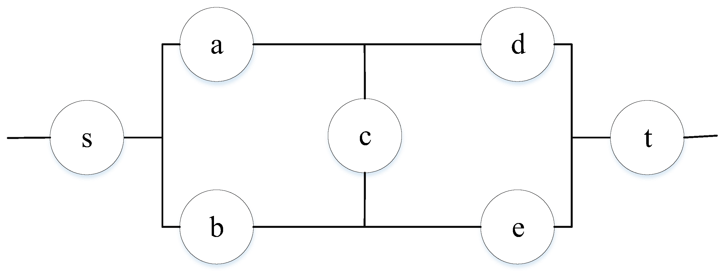
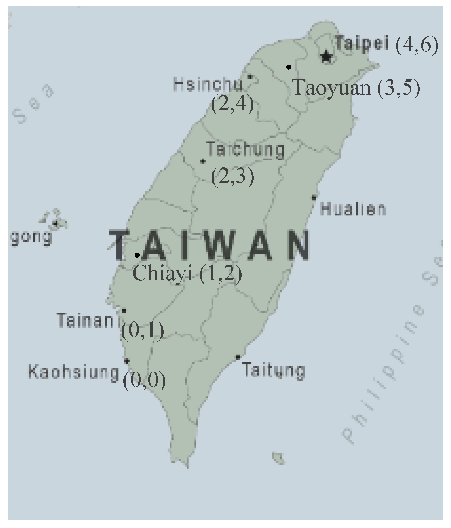
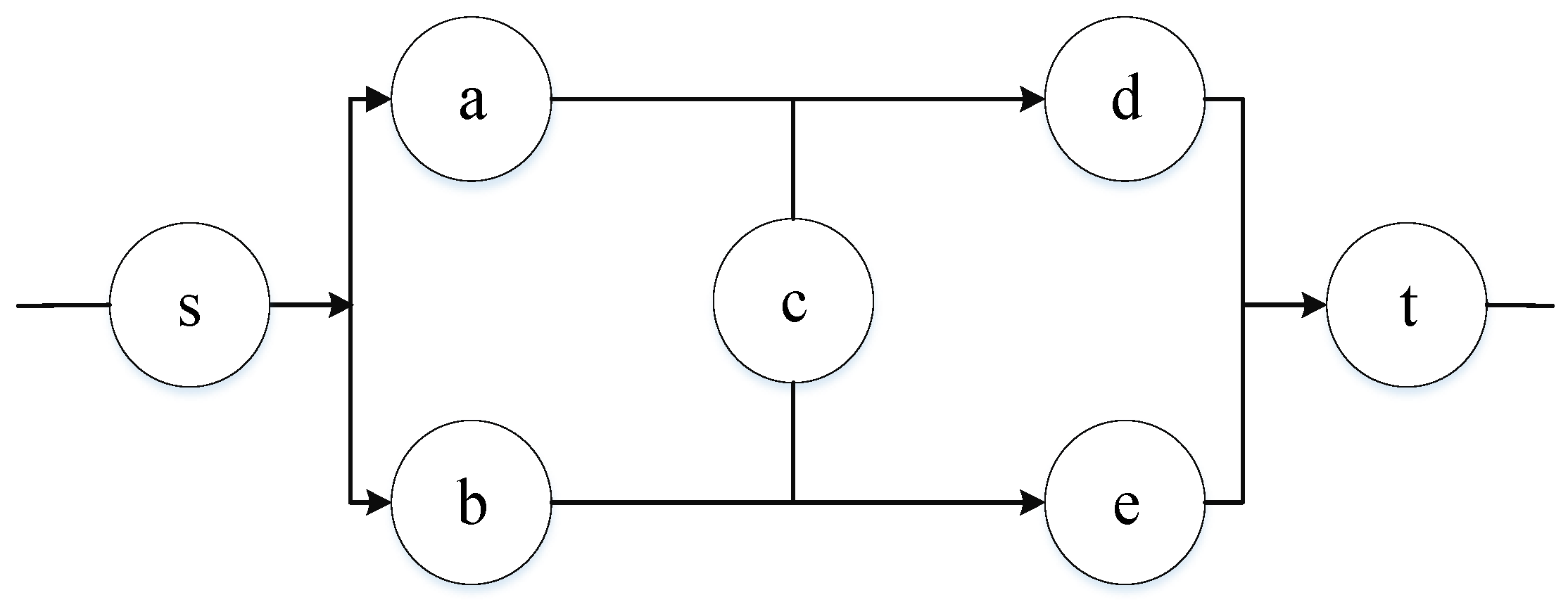
Moreover, considering that the current research on MFN reliability has been less applied to a bridge network (as shown in Figure 1), in which the symbols a, b, c, d, and e represent five nodes that are connected by edges, this study is based on a bridge network and expands it to add a source node and a sink node (as shown in Figure 2), in which the symbols s and t represent the source node and the sink node, respectively. The multi-stage traffic network map used in this study is an innovative network diagram. 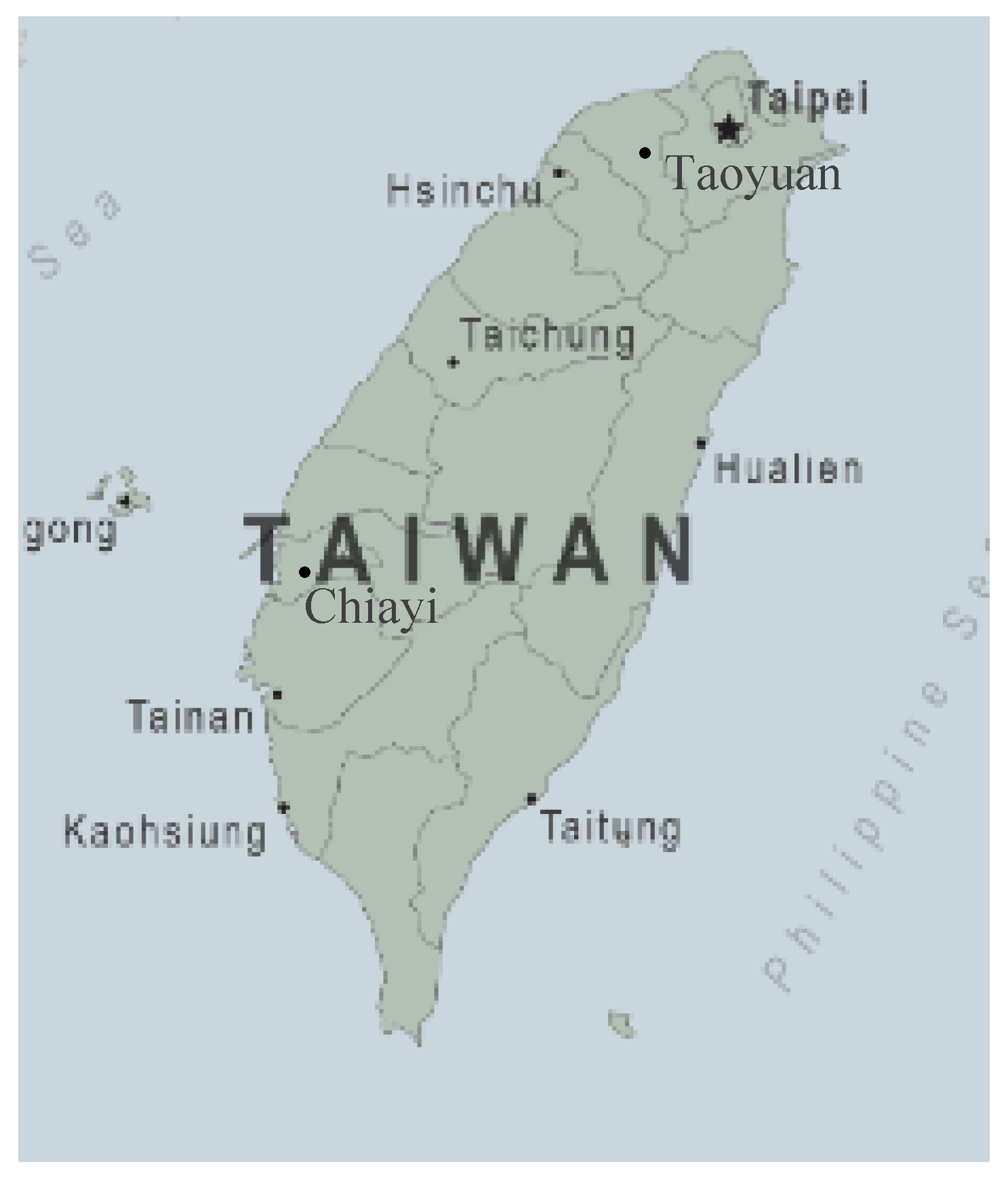This study-extended bridge network is shown in Figure 2 as an example, where it has been applied to logistics distribution from north to south in Taiwan to evaluate MFN reliability considering road conditions with different speed limits.

The remaining sections of the manuscript are structured as follows: Section 2 presents a literature review. A description of the studied problem is stated in Section 3. The proposed method is based on the basic d-MP algorithm that is introduced in Section 4. The proposed algorithm is shown in Section 5. Section 6 presents a numerical example. Finally, the conclusions are discussed in Section 7.

2. Literature Review

2.1. Intelligent Logistics

The construction of intelligent logistics with intelligent wireless sensing is a global trend; thus, the related works on intelligent logistics are included in a literature review in this section. The related works on intelligent logistics can be classified into the following types:

• Intelligent logistics in the Internet of Things (IoT)

Liu et al. developed the IoT by implementing intelligent logistics, big data analysis, and the machine learning method [20]. Humayun et al. proposed the IoT to enhance intelligent logistics and smart transportation [21]. In addition, Spandonidis et al. developed an intelligent IoT to improve the logistics of air cargo [22].

2.

Intelligent logistics in numerous topics, such as routing layout, robotics, smart warehousing, and supply chain

Li et al. studied the routing design for the intelligent logistics of the food field [23]. Wen et al. presented robotics to apply in intelligent logistics [24]. Pandian applied intelligent logistics to smart warehousing [25]. In addition, Riahi et al. introduced intelligent logistics for the supply chain [26].

3.

The review of intelligent logistics

Woschank et al. introduced a review of intelligent logistics [27]. Ding et al. concluded a review of intelligent logistics in the IoT [28]. Toorajipour et al. presented a review of intelligent logistics for the supply chain [29]. In addition, Feng and Ye provided a review of intelligent logistics management [30].

2.2. Reliability of Delivery

The reliability of delivery is addressed in greater detail by a survey of the related works regarding the d-MP, transport optimization, and reliability of delivery:

• The reliability of delivery regarding the d-MP

There are numerous works focusing on the reliability of delivery regarding the d-MP that consider different conditions, such as a two-terminal network [4], the delivery time [12], the turning angle [19], and various algorithms, including a method based on the Monte Carlo simulation method [5], a recursive algorithm [7], a new direct algorithm [9], etc.

2.

The reliability of delivery regarding transport optimization

Several works on the reliability of delivery regarding transport optimization are solved by numerous approaches, such as simplified swarm optimization (SSO) [13], real-time management [31], the path-based method [32], social engineering optimization (SEO), a combination of firefly and the simulated annealing (SA) approach [33], and production functions [34].

3.

The reliability of delivery

Moreover, many related works on the reliability of delivery were studied, such as the production network [14], allocation design [16], vehicle routing planning [35], task scheduling [36], power systems [37], social networks [38], the binary-state network [39], and the supply chain [40].

3. Problem Description

As stated in Section 2, the research gap between the existing approaches and the novel approach proposed in this manuscript contains the following two main points:

• This study proposes two different types of roads, and the speed limit of a road is used as the basis for distinguishing between the road types. There are few existing studies on the type of roads.
• In addition to the research in reference [19], fewer existing studies take turning angles into account, which is another focus of this study.

Therefore, the road type characteristics and the formula of the turning angle are stated in Section 3.1 and Section 3.2, respectively. In addition, according to the formula of the turning angle, the transportation distance and transportation lead time that are considered in this study are also introduced in Section 3.2.

3.1. Road Type Characteristics

The two different road types applied in this study, namely highways and slow roads, are represented by the notations Rd_h and Rd_g, respectively, and the analyses of their characteristics are shown in

Table 1. Transportation characteristics of two different road types.

Characteristics	Rdh	Rdg
Speed	Faster	Slower
Turning angle	Limited	Not limited
Transportation lead time at equal distances	Shorter	Longer
Vehicle loading capacity	Lower	Higher
Number of distributions of equal quantity	More	Less
Tolls	Charge	Non-charge

.

The problem in this study is solved based on the following assumptions:

• Only one truck delivers the goods.
• The loading capacity of each truck is W (unit weight).
• The turning angle is limited to less than 90 degrees when the truck is driving on Rd_h.
• There is no limit to the turning angle when the truck is driving on Rd_g.

The following information is further analyzed according to the transportation characteristics of the two different road types from Table 1:

• Transportation lead time at equal distances: The transportation lead time is longer for driving on Rd_g because the speed is slower, while the transportation lead time is shorter for driving on Rd_h because the speed is faster.
• Turning angle: The turning angle is not limited for driving on Rd_g because the speed is slower, and the turning angle of the truck can be large, while the turning angle is limited for driving on Rd_h because the speed is faster, and there is a danger of overturning the truck if the angle of the truck is too large.
• Vehicle loading capacity: The vehicle loading capacity is higher for driving on Rd_g because there is no weight limit, while the vehicle loading capacity is lower for driving on Rd_h because there is a weight limit.
• Number of distributions of equal quantity: The number of distributions is less for driving on Rd_g because the vehicle loading capacity is higher, and the amount of heavier cargo can be loaded on each departure truck, while the number of distributions is greater for driving on Rd_h because the vehicle loading capacity is lower, and a small (light) quantity of cargo can be loaded on each truck. The following example offers a description:

Example. Suppose that three (unit weight) goods need to be delivered, the load weight limits are three (unit weight) and two (unit weight) for vehicles driving on Rd_h and Rd_g, respectively.

Solution: The vehicle needs to run three times while driving on Rd_h to transport all three (unit weight) goods to the destination because the first one can only carry two (unit weight) of the goods. Then, the second requires empty vehicles to return from the destination, and the third picks up the remaining good (unit weight) from the source node and transports it to the destination.

The vehicle only needs to run one time while driving on Rd_g to transport all three (unit weight) goods to the destination.

3.2. Formula of Turning Angle, Transportation Distance, and Transportation Lead Time

The turning angle is not limited for driving on Rd_g; however, the turning angle is limited for driving on Rd_h. Here, the 2D multistate flow angle network proposed by Wu [19] is applied, and thus, the turning angle can be referred to the cosine trigonometric function as Equation (1), and the Euclidean distance formula is shown in Equation (2). Moreover, the law of the turning angle is proposed as shown in Lemma 1 and Property 1.

$$\cos \theta =(a^2+b^2-c^2)/2ab$$

(1)

where θ is the angle between both sides of a and b and the diagonal sides of c.

$$d(x_{(i,j)},y_{(l,k)})=\sqrt{{(x_i-y_l)}^2+{(x_j-y_k)}^2}$$

(2)

where x_(i,j) and y_(l,k) is the coordinate of two points on the (x, y) plane.

Lemma 1.

Let the turning angle be an exterior angle. The cosine value of the turning angle equals the reverse side of the cosine value of the interior angle where the interior angle plus the exterior angle equals 180°, i.e., cos θ = −cos (180° − θ) for the turning angle equals θ.

Property 1.

For the turning angle θ ∈ (0, π), cos θ shows a decrease when θ increases.

The speed is slow when the truck is driving on a slow road (Rd_g); thus, it is assumed that the transportation lead time requires 1.5 h for one unit of transport distance. In contrast, the speed is fast when the truck is driving on the highway (Rd_h); thus, it is assumed that the transportation lead time is only 0.5 h for one unit of transport distance. Therefore, the transportation lead time of a single trip for two kinds of roads can be expressed by Equations (3) and (4), respectively.

T_g = 1.5 (L)

(3)

T_h = 0.5 (L)

(4)

where T_g represents the transportation lead time while driving on Rd_g (hours), T_h is the transportation lead time while driving on Rd_h (hours), and L is the transport distance.

4. The Basic d-MP Algorithm

The proposed method is based on the basic d-MP algorithm, introduced in Section 4.

The d-MP flow can find by the d-MP algorithm [4], as shown in Theorem 1.

Theorem 1.

Any state vector of system X = (3.5x₁, x₂, …, x_n) is a d-MP candidate, i.e., the maximum flow of the system M(X) = d, if and only if the flow vector (f₁, f₂, …, f_p) satisfies the following terms, i.e., Equations (5)–(7).

$${\displaystyle \sum _{j=1}^p{f}_j=d}$$

(5)

$$f_j\le F\hspace{1em}for j=1, 2, \dots , p$$

(6)

$$x_i=x_i(e_i)={\displaystyle \sum _{j=1}\left\{f_j\right|e_i\in P_j\}\le }M(e_i) for i=1, 2, \dots , n$$

(7)

where F is the maximum capacity of the flow, and M(e_i) is the maximum flow of the edge e_i.

In Theorem 1, Equation (5) is the total flow of each MP, and Equations (6) and (7) are the constraints of the flow of each MP and each edge, respectively.

5. The Algorithm

The proposed method is shown in Section 5.1 through Section 5.4.

As stated in Section 2, one of the major research gaps between the existing approaches and the novel approach proposed in this manuscript is that this study proposes two different types of roads. Therefore, the distinction between the existing d-MP algorithm and the improvements proposed in this manuscript is arranged in the following two points:

• For a truck driving on a highway (Rd_h), the (d;θ,W,T)-MP algorithm, which is limited by the turning angle (θ), vehicle loading capacity (W), and transportation lead time (T), can be found by extension of the d-MP algorithm and is shown in Theorem 3 [19], which was clearly introduced in Section 5.2.
• For a truck driving on a slow road (Rd_g), the (d;W,T)-MP algorithm, which is limited by the vehicle loading capacity (W) and transportation lead time (T), can be found by extension of the d-MP algorithm and is shown in Theorem 5 [19], which was clearly introduced in Section 5.3.

The MFN reliability of the cargo distribution is evaluated based on the famous d-MP algorithm [4] first to find all feasible minimum paths (MPs), as described in Section 4. The turning angle is limited for driving on Rd_h; thus, the d-MP algorithm is expanded to the (d; A)-MP algorithm, which is limited by the turning angle and is described in detail in Section 5.1. Trucks driving on slow roads and highways are subject to different constraints, as explained in Section 5.2 and Section 5.3, respectively. Finally, Section 5.4 describes the calculation of MFN reliability.

5.1. d-MP with Angle Constraint

The (d;θ)-MP algorithm, which is limited by the turning angle denoted as θ, can be found by extension of the d-MP algorithm and is shown in Theorem 2 [19].

Theorem 2.

Any state vector of a system considering the angle window X_∠θ = (x₁, x₂, …, x_n) is a (d;θ)-MP candidate, i.e., the maximum flow of the system M(X_∠θ) = d, if and only if the flow vector (f₁, f₂, …, f_p) satisfies the following terms, i.e., Equations (5) and (7)–(9).

$$f_j\le F_{\angle {\theta }_j}\hspace{1em}for j=1, 2, \dots , p$$

(8)

$${\displaystyle \sum _{j=1}\left\{f_j\right|\angle \theta \in P_j\}\le }{M}_{\angle \theta }$$

(9)

where ∠θ is denoted as the angle θ; F_∠θ is the maximum capacity of the flow considering the angle window; M(e_i) is the maximum flow of the edge e_i; and M_∠θ is the maximum flow of e_i, limited by the angle window of ∠θ.

In Theorem 2, Equation (5) is the total flow of each MP with the angle θ, and Equations (6)–(9) are the constraints of the flow of each MP with the angle θ, each edge, and each angle.

5.2. (d;θ,W,T)-MP

For a truck driving on the highway (Rd_h), the (d;θ,W,T)-MP algorithm, which is limited by the turning angle (θ), vehicle loading capacity (W), and transportation lead time (T), can be found by extension of the d-MP algorithm and is shown in Theorem 3 [19].

Theorem 3.

Any state vector of a system considering the constraints of the turning angle, vehicle loading capacity, and transportation lead time X_∠θ,W,T = (x₁, x₂, …, x_n) is a (d;θ,W,T)-MP candidate, i.e., the maximum flow of the system M(X_∠θ,W,T) = d, if and only if the flow vector (f₁, f₂, …, f_p) satisfies the following terms, as shown in Equations (5) and (7)–(11).

$$w_i\le W\hspace{1em}for i=1, 2, \dots , n$$

(10)

$${\displaystyle \sum _{i=1}\{t(e_i)|e_i\in P_j\}\le }T$$

(11)

where w_i is the weight limit of the edge e_i, which was used to present the maximum vehicle loading capacity; t(e_i) is time spent driving on the edge e_i; W and T are the upper limitations of the maximum vehicle loading capacity and the total transportation lead time, respectively.

In Theorem 3, Equation (5) is the total flow of each MP, and Equations (7)–(11) are the constraints of the flow of each MP with the angle θ, each edge, each angle, the vehicle loading capacity, and the total transportation lead time.

Next, we check whether the state vector candidates are real state vectors in the MFN according to Theorem 4 [19].

Theorem 4.

The state vector candidate is a real state vector if and only if the cyclic direction does not exist in the system of the network.

5.3. (d;W,T)-MP

For the truck driving on the slow road (Rd_g), the (d; W,T)-MP algorithm, which is limited by the vehicle loading capacity (W) and transportation lead time (T), can be found by extension of the d-MP algorithm and is shown in Theorem 5 [19].

Theorem 5.

Any state vector of a system considering the constraints of the vehicle loading capacity and transportation lead time X = (x₁, x₂, …, x_n) is a (d;W,T)-MP candidate, i.e., the maximum flow of the system M(X) = d, if and only if the flow vector (f₁, f₂, …, f_p) satisfies the following terms, as shown in Equations (5)–(7), (10) and (11).

In Theorem 5, Equation (5) is the total flow of each MP, and Equations (6), (7), (10) and (11) are the constraints of the flow of each MP, each edge, the vehicle loading capacity, and the total transportation lead time.

Next, we also check whether the state vector candidates are real state vectors in the MFN according to Theorem 4 [19].

5.4. MFN Reliability

The MFN reliability, denoted as R, is calculated by the inclusion–exclusion method [19], as shown in Equation (12):

$$\mathrm{R}={\displaystyle \sum _{i=1}^{v}P}(x_i)-{\displaystyle \sum _{j=2}^v{\displaystyle \sum _{i=1}^{j-1}P(x_i\cap x_j)+{\displaystyle \sum _{j=3}^v{\displaystyle \sum _{i=2}^{j-1}{\displaystyle \sum _{k=1}^{i-1}P(x_i\cap x_j\cap x_k)+\dots +{(-1)}^{v+1}P(x_1\cap x_2\cap \dots \cap x_v)}}}}}$$

(12)

where x₁, x₂, …, x_v are the real (d;θ,W,T)-MP or the real (d;W,T)-MP.

6. Numerical Example

6.1. Description of Example

This study takes the extended bridge network in Figure 2 as an example and applies it to logistics distribution from north to south in Taiwan. Taipei, Hsinchu, Taoyuan, Taichung, Chiayi, Tainan, and Kaohsiung are seven major cities with large cargo, flows from north to south in Taiwan; there are many companies, industrial manufacturers, warehouses, and ports located in these seven cities. The locations of these seven cities are shown in Figure 3 [41].

The types of roads connecting these seven cities are divided mainly into two types, i.e., highways (Rd_h) and slow roads (Rd_g). Therefore, from north to south in Taiwan, trucks can choose to drive on Rd_h or Rd_g. The delivery of goods starts at the northernmost source point of Taipei, passes through Taoyuan, Hsinchu, and Taichung and then through Taichung via Chiayi and Tainan, and finally delivers the goods to the southernmost destination, Kaohsiung.

From the cargo transportation routes of the aforementioned seven major cities in Taiwan, the extended bridge network in Figure 2 can be applied to the logistics distribution from north to south in Taiwan. The nodes s and t stand for the source node, i.e., Taipei, and the sink node, i.e., Kaohsiung, respectively. The intermediate nodes a through e stand for Taoyuan, Hsinchu, Taichung, Chiayi, and Tainan, respectively. Hence, the complete directed MFN is shown in Figure 4.

The plane coordinates of the seven cities in Taiwan are marked as Taipei (s): (4,6), Taoyuan (a): (3,5), Hsinchu (b): (2,4), Taichung (c): (2,3), Chiayi (d): (1,2), Tainan (e): (0,1), and Kaohsiung (t): (0,0), respectively, as shown in Figure 5.

Each edge in the MFN of Figure 4 is numbered as shown in Figure 6, in which the edge via Taichung (node c) is bidirectional, containing e₅ and e₆, while the other edges of other cities are unidirectional.

As described in Section 3, the types of roads in Taiwan’s seven major cities, from north to south, include slow road (Rd_g) and highway (Rd_h) options. Assume that the load weight limit for a vehicle driving on Rd_h is two (unit weight). Although there is no load weight limit of a vehicle driving on Rd_g, it is assumed that the truck weight limit is three (unit weight) no matter the vehicle driving on Rd_h or Rd_g. The probability of the loading capacity of the two road types for each edge of Figure 6 is given in

Table 2. The probability of the loading capacity of the two road types for each edge of Figure 6.

Edge	Capacity	Probability Rdh	Probability Rdg	Edge	Capacity	Probability Rdh	Probability Rdg
e1	3	0	0.7	e5	3	0	0.8
	2	0.9	0.1		2	0.8	0.05
	1	0.05	0.1		1	0.1	0.1
	0	0.05	0.1		0	0.1	0.05
e2	3	0	0.7	e6	3	0	0.85
	2	0.7	0.1		2	0.85	0.05
	1	0.2	0.1		1	0.1	0.05
	0	0.1	0.1		0	0.05	0.05
e3	3	0	0.8	e7	3	0	0.85
	2	0.8	0.1		2	0.7	0.05
	1	0.1	0.05		1	0.15	0.05
	0	0.1	0.05		0	0.15	0.05
e4	3	0	0.9	e8	3	0	0.85
	2	0.9	0.05		2	0.8	0.05
	1	0.05	0.05		1	0.1	0.05
	0	0.05	0		0	0.1	0.05

.

6.2. Drive on Rd_h

In this study, the example plans to distribute three units of goods from the city of Taipei in northern Taiwan, i.e., the source node s, to Kaohsiung in the south, i.e., the sink node t as shown in the MFN in Figure 6. The plane coordinates of the seven cities in Taiwan are given in Figure 5.

First, the choice of the truck to drive on the highway (Rd_h) is limited to those with less than a 90-degree turning angle, a vehicle loading capacity that does not exceed two units of weight, and a total transport lead time of less than 12 h. The calculation process of the MFN reliability is as follows:

Step 1.

Find all MPs in Figure 6. A total of four MPs were found as below. P1 = {e1, e3, e7}, P2 = {e1, e5, e8}, P3 = {e2, e4, e8}, P4 = {e2, e6, e7}

Step 2.

Calculate the length between nodes of each MP using the coordinates in Figure 5 and Equation (2). This is shown in Table 3. Length between nodes of each MP. P1 P2 P3 P4 Nodes Length Nodes Length Nodes Length Nodes Length s→a 1.414214 s→a 1.414214 s→b 2.828427 s→b 2.828427 a→d 4.242641 a→c 2.236068 b→e 3.605551 b→c 1 s→d 5 s→c 3.605551 s→e 6.403124 s→c 3.605551 d→t 2.236068 c→e 2.828427 e→t 1 c→d 2.236068 a→t 5.830952 a→e 5 b→t 4.472136 b→d 2.236068 e→t 1 d→t 2.236068 c→t 3.605551 c→t 3.605551 .

Step 3.

The cosine values of angles using Equation (1). This is shown in Table 4. Cosine values of angles. P1 P2 P3 P4 Angle Cosine Angle Cosine Angle Cosine Angle Cosine cos∠sad −0.41667 cos∠sac −0.94868 cos∠sbe −0.98058 cos∠sbc −0.70711 cos∠adt −0.57975 cos∠ace −0.94868 cos∠bet −0.83205 cos∠bcd 0.223607 cos∠cet −0.70711 cos∠cdt −0.3 .

In this experiment, driving on the highway only qualifies if the turning angle is less than 90 degrees. Using the information in Table 4, the turning angles of the four paths P₁ through P₄ are all less than 90 degrees; thus, all are qualified paths.

Step 4.

Driving on Rdh, the maximum load per truck is two (unit weight), so the truck has to run back and forth three times to complete the delivery of three units of goods, i.e., two units for the first trip, one return trip to empty the truck, and the final time (the third trip) is to deliver the last unit. Therefore, the above information is used to calculate a single transport lead time using Equation (4) and is listed in Equations (13)–(16) for P1 through P4, respectively. The relevant calculation results are shown in Table 5. Transport lead time on Rdh. MPs P1 P2 P3 P4 Type of road Rdh Rdh Rdh Rdh Maximum load/each trip 2 2 2 2 Times to complete the delivery of 3 units of goods 3 3 3 3 Single transport lead time 3.946462 3.739355 3.716989 4.150282 Total transport lead time 11.839386 11.21806 11.15097 12.450846 . The total transport lead time of each MP is the number of turns multiplied by the single transport lead time, as shown in the sixth column of Table 5.

P₁: T_h = 0.5 (L) = 0.5(1.414214 + 4.242641 + 2.236068) = 3.946462 (h)

(13)

P₂: T_h = 0.5 (L) = 0.5(1.414214 + 2.236068 + 2.828427 + 1) = 3.739355 (h)

(14)

P₃: T_h = 0.5 (L) = 0.5(2.828427 + 3.605551 + 1) = 3.716989 (h)

(15)

P₄: T_h = 0.5 (L) = 0.5(2.828427 + 1 + 2.236068 + 2.236068) = 4.150282 (h)

(16)

Step 5.	P4 is deleted because the total transport lead time is greater than 12 (h).
Step 6.	Find the flow vector of (d;W,T)-MP∠A = (3;2,12)-MP∠90 via Equations (17)–(20) listed below.

$${\displaystyle \sum _{j=1}^3{f}_j=3}$$

(17)

$$f_1\le F_{A1}=2$$

(18)

$$f_2\le F_{A2}=2$$

(19)

$$f_3\le F_{A3}=2$$

(20)

A total of seven flow vectors for (3;2,12)-MP_∠90 are found: (2,1,0), (2,0,1), (1,2,0), (1,0,2), (1,1,1), (0,2,1), and (0,1,2).

Step 7.

Transfer the flow vectors of (3;2,12)-MP∠90 to the state vector candidates of (3;2,12)-MP∠90, which has been verified to be a real vector. This is shown in Table 6. The real state vector of (3;2,12)-MP∠90. Flow Vectors of (3;2,12)-MP∠90 State Vector Candidates of (3;2,12)-MP∠90 Capacity of Edge ≤ 2 Verify by Theorem 4 Real State Vectors of (3;2,12)-MP∠90 (2,1,0) (3,0,2,0,1,0,2,1) N (2,0,1) (2,1,2,1,0,0,2,1) Y N Y (1,2,0) (3,0,1,0,2,0,1,2) N (1,0,2) (1,2,1,2,0,0,1,2) Y N Y (1,1,1) (2,1,1,1,1,0,1,2) Y N Y (0,2,1) (2,1,0,1,2,0,0,3) N (0,1,2) (1,2,0,2,1,0,0,3) N .

Step 8.

Use the information about the real state vectors of (3;2,12)-MP∠90 obtained in Table 6 and of the distribution of the capacity listed in Table 2 to calculate the system reliability of the transfer of three units of goods driving on Rdh from Taipei to Kaohsiung, denoted as R(3;2,12)-MP∠90 in the multi-flow network of Figure 6. R(3;2,12)-MP∠90 was obtained by the inclusion–exclusion principle shown in Equation (21).

$$\begin{array}{ll}{\mathrm{R}}_{(3;2,12)-\mathrm{MP}\angle 90}& ={\displaystyle \sum _{i=1}^{3}P(x_i)-{\displaystyle \sum _{j=2}^3{\displaystyle \sum _{i=1}^{j-1}P(x_i\cap x_j)+{(-1)}^{3+1}P(}}}{x}_i\cap x_j\cap x_k)\\ & =1.665198-1.411024+0.4210704\\ & =0.675244\end{array}$$

(21)

The reliability equals 67.5244% for the distribution of three units of goods from Taipei in northern Taiwan, i.e., the source node s, to Kaohsiung in the south, i.e., the sink node t, as shown in the MFN for driving on the highway (Rd_h) in Figure 6.

6.3. Drive on Rd_g

Secondly, the choice of truck to drive on the slow roads (Rd_g) is limited to the vehicle loading capacity and cannot exceed three units of weight. The total transport lead time is less than 12 h, and the calculation process of the MFN reliability is as follows:

Step 1.	Find all MPs in Figure 6. A total of four MPs were found as below. P1 = {e1, e3, e7}, P2 = {e1, e5, e8}, P3 = {e2, e4, e8}, P4 = {e2, e6, e7}
Step 2.	The length between nodes of each MP is calculated using the coordinates in Figure 5 and Equation (2), as shown in Table 3.
Step 3.	The above information is used to calculate the single transport lead time using Equation (3) and is listed in Equations (22)–(25) for P1 through P4, respectively. The relevant calculation results are shown in Table 7. Transport lead time on Rdg. MPs P1 P2 P3 P4 Type of road Rdg Rdg Rdg Rdg Maximum load/each trip 3 3 3 3 Times to complete the delivery of 3 units of goods 1 1 1 1 Single transport lead time 11.83938 11.21806 11.15097 12.45084 Total transport lead time 11.83938 11.21806 11.15097 12.45084 . The total transport lead time of each MP is the number of turns multiplied by the single transport lead time, as shown in the sixth column of Table 7.

P₁:T_g = 1.5 (L) = 1.5(1.414214 + 4.242641 + 2.236068) = 11.83938 (h)

(22)

P₂:T_g = 1.5 (L) = 1.5(1.414214 + 2.236068 + 2.828427 + 1) = 11.21806 (h)

(23)

P₃:T_g = 1.5 (L) = 1.5(2.828427 + 3.605551 + 1) = 11.15097 (h)

(24)

P₄:T_g = 1.5 (L) = 1.5(2.828427 + 1 + 2.236068 + 2.236068) = 12.45084 (h)

(25)

Step 4.	P4 is deleted because the total transport lead time is greater than 12 (h).
Step 5.	Find the flow vector of (d;W,T)-MP = (3;3,12)-MP via Equations (26)–(28) as below.

$${\displaystyle \sum _{j=1}^2{f}_j=3}$$

(26)

$$f_1\le F=3$$

(27)

$$f_2\le F=3$$

(28)

A total of 10 flow vectors for (3;3,12)-MP are found: (3,0,0), (0,3,0), (0,0,3), (2,1,0), (2,0,1), (1,2,0), (1,0,2), (1,1,1), (0,2,1), and (0,1,2).

Step 6.

Transfer the flow vectors of (3;3,12)-MP to the state vector candidates of (3;2,12)-MP, which are verified by Theorem 4 to check whether they are real vectors. This is shown in Table 8. The real (3;3,12)-MP state vector. Flow Vectors of (3;3,12)-MP State Vector Candidates of (3;3,12)-MP Verify by Theorem 4 Real State Vectors of (3;3,12)-MP (3,0,0) (3,0,3,0,0,0,3,0) N Y (0,3,0) (3,0,0,0,3,0,0,3) N Y (0,0,3) (0,3,0,3,0,0,0,3) N Y (2,1,0) (3,0,2,0,1,0,2,1) N Y (2,0,1) (2,1,2,1,0,0,2,1) N Y (1,2,0) (3,0,1,0,2,0,1,2) N Y (1,0,2) (1,2,1,2,0,0,1,2) N Y (1,1,1) (2,1,1,1,1,0,1,2) N Y (0,2,1) (2,1,0,1,2,0,0,3) N Y (0,1,2) (1,2,0,2,1,0,0,3) N Y .

Step 7.

Use the information about the real (3;3,12)-MP state vectors obtained in Table 8 and the distribution of the capacity listed in Table 2 to calculate the system reliability of the transfer of three units of goods driving on Rdg from Taipei to Kaohsiung, denoted as R(3;3,12)-MP, in the multi-flow network of Figure 6. R(3;3,12)-MP was obtained by the inclusion–exclusion principle, as shown in Equation (29).

$$\begin{array}{l}{R}_{(3;3,15)-\mathrm{MP}}\\ ={\displaystyle \sum _{i=1}^{10}P(x_i)-{\displaystyle \sum _{j=2}^{10}{\displaystyle \sum _{i=1}^{j-1}P(x_i\cap x_j)+{\displaystyle \sum _{j=3}^{10}{\displaystyle \sum _{i=2}^{j-1}{\displaystyle \sum _{k=1}^{i-1}P(x_i\cap x_j\cap x_k)}}}}}}+\dots +{(-1)}^{10+1}P(x_1\cap x_2\cap \dots \cap x_{10})\\ =5.220234-17.42824+38.9189-60.4683+66.53501-51.8076+27.93726\\ -9.983585+2.132992-0.2039184\\ =0.852753\end{array}$$

(29)

The reliability equals 85.2753% to distribute three units of goods from Taipei in northern Taiwan, i.e., the source node s, to Kaohsiung in the south, i.e., sink node t, as the MFN, as shown in Figure 6, for driving on the slow roads (Rd_g).

7. Conclusions

The contribution of this study is to propose a new multistate flow network diagram with the complexity of the actual transportation road network to help enhance the construction of intelligent wireless sensing in intelligent logistics. The complex multistate flow network proposed in this study can be used to simulate the logistics distribution network from north to south in Taiwan.

Road type (type of edge) has rarely been discussed in the existing reliability research on the multistate flow network, so that is proposed by this study for discussion. The reliability of the multistate flow network is evaluated by studying trucks traveling on highways and slow-speed roads, two road types with different speeds and different constraints. These are applied to the delivery of goods on the multistate flow network from north to south in Taiwan as an actual case to discuss. The results of this study show that trucks traveling on highways and slow-speed roads have similar logistics reliability for the same unit of goods distributed. This also echoes the actual situation. In the transportation of goods in Taiwan, it is not difficult to find that there are trucks of various companies driving through both types of roads for the distribution of goods.

In today’s business environment, the competition has become increasingly fierce, and the reliability of the logistics distribution is also one of the factors for the success of each enterprise. Therefore, the research planning and research results of this study can be effectively provided for academic and practical reference.

For continuation in further research, automated data acquisition of intelligent logistics is being considered for study in future work.

In the future study, weight restrictions for trucks and heavy goods vehicles on all public roads can be considered to ensure public safety and to relocate heavy road transport to main roads and highways that link main logistic centers and bypass cities and heavily populated areas. Furthermore, in future work, the assumption that “The turning angle is limited by less than 90 degrees when the truck is driving in highways” can be considered for deletion because there are fewer curves or junctions on major roads and highways than on local roads.

The model for analyzing and optimizing the delivery of goods by trucks can be planned to be more universal, and certain restrictions and parameters of individual routes can be included as weights, or certain attributes can be assigned to the edges between nodes in a future study. More than two types of roads (national highways, provincial highways, expressways, non-urban roads, urban roads, etc.) can be studied based on this work in the future. Moreover, various patterns of vehicle movement can be considered in future work. In addition, in this work in the future, the edges of the network in the model can take into account the real length of the route instead of the length between the nodes calculated from the coordinates as the distance between two points using Formula (2).

References

1. Lee, S.H. Reliability evaluation of a flow network. IEEE Trans. Reliab. 1980, 29, 24–26. [Google Scholar] [CrossRef]
2. Bai, G.; Tian, Z.; Zuo, M.J. Reliability evaluation of multistate networks: An improved algorithm using state-space decomposition and experimental comparison. IISE Trans. 2018, 50, 407–418. [Google Scholar] [CrossRef]
3. Chen, S.G.; Lin, Y.K. An Improved Merge Search Approach to Evaluate Reliability in Multistate Network Systems. IEEE Trans. Reliab. 2021, 71, 382–389. [Google Scholar] [CrossRef]
4. Bai, G.; Zuo, M.J.; Tian, Z. Search for all d-MPs for all d levels in multistate two-terminal network. Reliab. Eng. Syst. Saf. 2015, 142, 300–309. [Google Scholar] [CrossRef]
5. EI Khadiri, M.; Yeh, W.C. An efficient alternative to the exact evaluation of the quickest path flow network reliability problem. Comput. Oper. Res. 2016, 76, 22–23. [Google Scholar] [CrossRef]
6. Levitin, G. Reliability of acyclic multi-state networks with constant transmission characteristics of lines. Reliab. Eng. Syst. Saf. 2002, 78, 297–305. [Google Scholar] [CrossRef]
7. Bai, G.; Tian, Z.; Zuo, M.J. An improved algorithm for finding all minimal paths in a network. Reliab. Eng. Syst. Saf. 2016, 150, 1–10. [Google Scholar] [CrossRef]
8. Ramirez-Marquez, J.E.; Coit, D.W.; Tortorella, M. A generalized multistate-based path vector approach to multistate two-terminal reliability. IIE Trans. 2006, 38, 477–488. [Google Scholar] [CrossRef]
9. Yeh, W.C. Novel Direct Algorithm for Computing Simultaneous All-level Reliability of Multistate Flow Networks. Reliab. Eng. Syst. Saf. 2022, 225, 108623. [Google Scholar] [CrossRef]
10. Yeh, W.C. New method in searching for all minimal paths for the directed acyclic network reliability problem. IEEE Trans. Reliab. 2016, 65, 1263–1270. [Google Scholar] [CrossRef]
11. Yeh, W.C. A squeezed artificial neural network for the symbolic network reliability functions of binary-state networks. IEEE Trans. Neural Netw. Learn. Syst. 2016, 28, 2822–2825. [Google Scholar] [CrossRef] [PubMed]
12. Lin, Y.K.; Huang, C.F.; Liao, Y.C.; Yeh, C.C. System reliability for a multistate intermodal logistics network with time windows. Int. J. Prod. Res. 2017, 55, 1957–1969. [Google Scholar] [CrossRef]
13. Yeh, W.C.; Tan, S.Y. Simplified Swarm Optimization for the Heterogeneous Fleet Vehicle Routing Problem with Time-Varying Continuous Speed Function. Electronics 2021, 10, 1775. [Google Scholar] [CrossRef]
14. Lin, Y.K.; Chang, P.C.; Yeng, L.C.L.; Huang, S.F. Bi-objective optimization for a multistate job-shop production network using NSGA-II and TOPSIS. J. Manuf. Syst. 2019, 52, 43–54. [Google Scholar] [CrossRef]
15. Ramirez-Marquez, J.E.; Coit, D.W. Multi-state component criticality analysis for reliability improvement in multi-state systems. Reliab. Eng. Syst. Saf. 2007, 92, 1608–1619. [Google Scholar] [CrossRef]
16. Taboada, H.A.; Espiritu, J.F.; Coit, D.W. Design allocation of multistate series-parallel systems for power systems planning: A multiple objective evolutionary approach. Proc. Inst. Mech. Eng. Part O J. Risk Reliab. 2008, 222, 381–391. [Google Scholar] [CrossRef]
17. Hao, Z.; Yeh, W.C.; Hu, C.F. A Novel Multistate Minimal Cut Vectors Problem and Its Algorithm. IEEE Trans. Reliab. 2019, 68, 291–301. [Google Scholar] [CrossRef]
18. He, M.F.; Hao, Z.F.; Yeh, W.C.; Kuo, C.C.; Xiong, N.N.; Shiue, Y.R. Quickest Multistate Flow Networks with the Deterioration Effect. IEEE Access 2020, 8, 145535–145541. [Google Scholar] [CrossRef]
19. Wu, H.S. A Novel 2D Binary-State Angle Network/2D Multi-State Flow Angle Network and the Reliability Evaluation. Master’s Thesis, National Tsing Hua University, Hsinchu, Taiwan, 2015. [Google Scholar]
20. Liu, C.; Feng, Y.; Lin, D.; Wu, L.; Guo, M. Iot based laundry services: An application of big data analytics, intelligent logistics management, and machine learning techniques. Int. J. Prod. Res. 2020, 17, 5113–5131. [Google Scholar] [CrossRef]
21. Humayun, M.; Jhanjhi, N.Z.; Hamid, B.; Ahmed, G. Emerging Smart Logistics and Transportation Using IoT and Blockchain. IEEE Internet Things Mag. 2020, 3, 58–62. [Google Scholar] [CrossRef]
22. Spandonidis, C.; Sedikos, E.; Giannopoulos, F.; Petsa, A.; Theodoropoulos, P.; Chatzis, K.; Galiatsatos, N. A Novel Intelligent IoT System for Improving the Safety and Planning of Air Cargo Operations. Signals 2022, 3, 95–112. [Google Scholar] [CrossRef]
23. Li, Y.; Chu, F.; Feng, C.; Chu, C.; Zhou, M.C. Integrated Production Inventory Routing Planning for Intelligent Food Logistics Systems. IEEE Trans. Intell. Transp. Syst. 2019, 20, 867–878. [Google Scholar] [CrossRef]
24. Wen, J.; He, L.; Zhu, F. Swarm robotics control and communications: Imminent challenges for next generation smart logistics. IEEE Commun. Mag. 2018, 56, 102–107. [Google Scholar] [CrossRef]
25. Pandian, A.P. Artificial Intelligence Application in Smart Warehousing Environment for Automated Logistics. J. Artif. Intell. Capsul. Netw. 2019, 1, 63–72. [Google Scholar] [CrossRef]
26. Riahi, Y.; Saikouk, T.; Gunasekaran, A. Artificial intelligence applications in supply chain: A descriptive bibliometric analysis and future research directions. Expert Syst. Appl. 2021, 173, 114702. [Google Scholar] [CrossRef]
27. Woschank, M.; Rauch, E.; Zsifkovits, H. A Review of Further Directions for Artificial Intelligence, Machine Learning, and Deep Learning in Smart Logistics. Sustainability 2020, 12, 3760. [Google Scholar] [CrossRef]
28. Ding, Y.; Jin, M.; Li, S.; Feng, D. Smart logistics based on the internet of things technology: An overview. Int. J. Logist. Res. Appl. 2021, 24, 323–345. [Google Scholar] [CrossRef]
29. Toorajipour, R.; Sohrabpour, V.; Nazarpour, A. Artificial intelligence in supply chain management: A systematic literature review. J. Bus. Res. 2021, 122, 502–517. [Google Scholar] [CrossRef]
30. Feng, B.; Ye, Q. Operations management of smart logistics: A literature review and future research. Front. Eng. Manag. 2021, 8, 344–355. [Google Scholar] [CrossRef]
31. Hrušovský, M.; Demir, E.; Jammernegg, W.; Woensel, T.V. Real-time disruption management approach for intermodal freight transportation. J. Clean. Prod. 2021, 280, 124826. [Google Scholar] [CrossRef]
32. Shen, H.; Liang, Y.; Shen, Z.J.M. Reliable Hub Location Model for Air Transportation Networks under Random Disruptions. Manuf. Serv. Oper. Manag. 2021, 23, 267–545. [Google Scholar] [CrossRef]
33. Goodarzian, F.; Kumar, V.; Ghasemi, P. A set of efficient heuristics and meta-heuristics to solve a multi-objective pharmaceutical supply chain network. Comput. Ind. Eng. 2021, 158, 107389. [Google Scholar] [CrossRef]
34. Abrorjon, X.E.; Umida, A.M. Assesment of metrological reliability of measurements using the method of producing functions. ACADEMICIA: Int. Multidiscip. Res. J. 2021, 11, 520–528. [Google Scholar]
35. Tan, S.Y.; Yeh, W.C. The Vehicle Routing Problem: State-of-the-Art Classification and Review. Appl. Sci. 2021, 11, 10295. [Google Scholar] [CrossRef]
36. Su, P.C.; Tan, S.Y.; Liu, Z.Y.; Yeh, W.C. A Mixed-Heuristic Quantum-Inspired Simplified Swarm Optimization Algorithm for scheduling of real-time tasks in the multiprocessor system. Appl. Soft Comput. 2022, 2022, 109807. [Google Scholar] [CrossRef]
37. Yeh, W.C.; Zhu, W.; Peng, Y.F.; Huang, C.L. A Hybrid Algorithm Based on Simplified Swarm Optimization for Multi-Objective Optimizing on Combined Cooling, Heating and Power System. Appl. Sci. 2022, 12, 10595. [Google Scholar] [CrossRef]
38. Yeh, W.C.; Zhu, W.; Huang, C.L. Reliability of Social Networks on Activity-on-Node Binary-State with Uncertainty Environments. Appl. Sci. 2022, 12, 9514. [Google Scholar] [CrossRef]
39. Yeh, W.C. Novel Self-Adaptive Monte Carlo Simulation Based on Binary-Addition-Tree Algorithm for Binary-State Network Reliability Approximation. Reliab. Eng. Syst. Saf. 2022, 228, 108796. [Google Scholar] [CrossRef]
40. Delfani, F.; Samanipour, H.; Beiki, H. A robust fuzzy optimisation for a multi-objective pharmaceutical supply chain network design problem considering reliability and delivery time. Int. J. Syst. Sci. Oper. Logist. 2022, 9, 155–179. [Google Scholar] [CrossRef]
41. Google Map. Available online: https://www.google.com.tw/maps/@23.4857501,120.0843006,7z?hl=en (accessed on 1 January 2022).
Figure 1. Bridge network.
Signals 03 00053 g001
Figure 2. The extended bridge network.
Signals 03 00053 g002
Figure 3. Taiwan map.
Signals 03 00053 g003
Figure 4. Directed MFN of goods shipped from northern Taiwan to the south.
Signals 03 00053 g004
Figure 5. Coordinates of seven cities in Taiwan.
Signals 03 00053 g005
Figure 6. Edge marked in the network.
Signals 03 00053 g006