Covariables of Soil-Forming Factors and Their Influence on pH Distribution and Spatial Variability

Abstract

The objectives of this study were to identify and rank the covariables of soil-forming factors that affect the distribution and spatial variability of pH in an agricultural area and to obtain a predictive map of soil pH. Samples of topsoil were obtained from different sites and taken to the laboratory, where they were prepared to determine the pH, organic matter, and percentages of particle size. In addition, the values of environmental covariables that affect pH were obtained. A database of the coordinates, laboratory results, and values of the covariables was constructed. Principal component analysis of the covariables was performed, and an analysis of the pH spatial structure was conducted and interpolated to obtain a predictive map of pH. Of the soil physical characteristics, the covariables clay and sand had a greater influence on the spatial behavior of pH with respect to the rest of the covariables of soil-forming factors, while human activity acted as a catalyst of the acidification process. Soil pH exhibited autocorrelation and moderate spatial dependence (66.7%) and was thus spatially predictable. The pH prediction map was accurate (RMSE = 0.158 and MEB = 0.020).

1. Introduction

The variability of edaphic characteristics and properties can be a function of soil-forming factors [1,2] and the relationship that occurs between the covariables (a variable or a group of variables that could predict the result under study) of these factors. One of the most important soil chemical characteristics derived from the relationships between these factors is pH [3]. pH is the negative logarithm, base 10, of the activity of H+, log (H+) [4,5], which determines whether soil is acidic (pH below 6.5, higher H+ concentration) or alkaline (pH above 7.5) [6]. Soil acidity is the greatest limitation to crop production [7]. The process of soil acidification can occur naturally as a result of its genesis or mode formation [8] or as the result of anthropic activity [9]. In this sense, acidification is one form of chemical soil degradation [10]. This situation becomes important in defining the factors that affect this process in a given region in the context of generating recommendations for the recovery and management of acid soils [11]. In this respect, diverse studies have established that the effect of factors on pH can differ depending on the location and scale of the study [12]. For example, it has been established that clay and organic matter (OM) content, precipitation and temperature, vegetation, and relief (the slope of the area where the soil is located), as well as humans, can affect pH [6]. In other words, pH is a function of edaphic or environmental covariables that constitute soil-forming factors. For this reason, the study of pH spatial behavior can be approached through the model Sc = f (SCORPAN) of McBratney et al. [13], where Sc is the soil attribute to be analyzed or modeled and is a function of the physical and chemical properties of the soil (S), the surrounding climate (C), the activity of organisms or vegetation (O), the attributes of the relief (R), the parent material (P), the geological age of the site (A), and the spatial position of the soil (N). However, studies that establish which sets of edaphic or environmental covariables have a greater influence on the spatial distribution of soil pH in a given area are scanty. Different studies, at a local level, have associated the behavior of pH with OM content [14] or the effect of pH on OM decomposition [15], with fertilizer application [16,17], with vegetation [11], with soil mineral particles [18], with the slope of the terrain, and with geological material [12,13,14,15,16,17,18,19]. Additionally, pH values, exchangeable acidity, and soil capacity for effective cationic exchange have been related to climate covariables (precipitation and temperature), as well as to the NDVI (normalized difference vegetation index), altitude, and some parameters of slope, at a regional level, to generate multivariate linear models and to obtain digital maps of soil attributes; models with coefficients of determination below 0.60 have been obtained [20]. Nonetheless, an explanation of how the covariables influence pH behavior and spatial distribution is incipient. In this context, determination of the spatial distribution and variability of soil characteristics is important for management in a region [21]. The evaluation of spatial distribution is possible using geostatistical techniques. These techniques permit the determination and interpretation of the behavior of soil variables over space [22]. The application of geostatistics to analyze the spatial structure of observations (variation in values as a function of their separation) facilitates spatial–temporal interpretation of the study variables in a region. There are different geostatistical methods for spatial estimations. One of the most used methods is the ordinary Kriging (OK) method. The effectiveness of OK has been demonstrated in the prediction of the spatial behavior of soil chemical characteristics [20]. However, this type of analysis by itself does not enable the identification of factors that intervene in the distribution of a variable of interest; it needs to be complemented. In this respect, principal component analysis (PCA) is another type of multivariate statistical analysis that has been shown to be useful in identifying groups of independent variables or covariables and in determining which of these has a greater influence on the spatial distribution of other edaphic variables [23]. Considering the above, it is likely that the analysis of pH spatial structure, complemented by PCA of the covariables of soil-forming factors that affect this edaphic variable, would be useful in identifying and ranking environmental covariables that affect pH spatial distribution and variability; this information could be useful for planning the management of soils with acidic pH in a region. Therefore, the objectives of this study were to establish the order of importance of the covariables of the soil-forming factors that influence pH spatial distribution and variability in an agricultural area of the municipality of Tlajomulco de Zúñiga, Jalisco, and to obtain a predictive map of soil pH.

2. Materials and Methods

This study was conducted on agricultural land (33,679.63 ha) in the municipality of Tlajomulco de Zúñiga, Jalisco, Mexico. This area is 49.3% of the total area of the municipality (68,247 ha) (Figure 1).

The site’s geology is made up of igneous rock from the Tertiary and alluvium from the recent Quaternary within the physiographic province of the Neo-Volcanic Belt. The predominant rocks are tuffs, which occupy 35.1% of the area; the rest are basalts (28.6%), andesites (6.7%), vitreous rocks (2.7%) and other types of rocks (2.3%). The alluvium is composed of fine pyroclastic particles (<4 mm in diameter), found in 25.6% of the municipality [24].

This region has a warm climate with summer rains ((A) C(w_o)) [25]. The mean annual temperature is 19.3 °C, while the average highs and lows are 28.6 and 10.1 °C, respectively. The mean annual precipitation is 782.7 mm [26].

The vegetation is composed of mesquite, scrub vegetation, and pine–oak forest. The soils are Cambisols, Feozem, Luvisols, and Vertisols. Land use is predominantly agricultural; maize is the main crop (49.4% of the area), although it is mostly planted in rainfed conditions [27]. This study comprised six stages, which are described below.

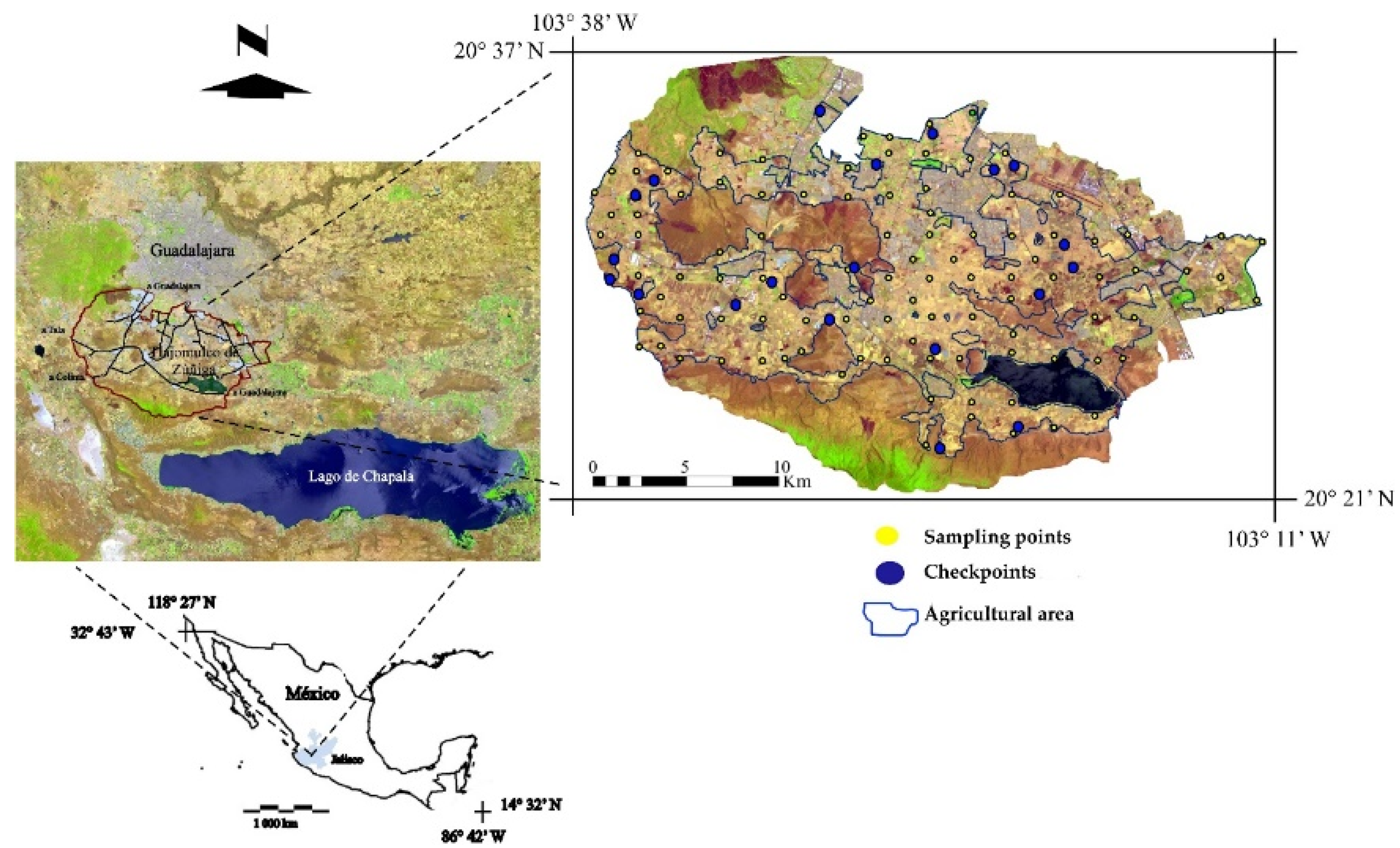
2.1. Location of Observation Points and Sample Collection

A grid (2500 $\times$ 2500 m) with UTM (Universal Transverse Mercator) projection was overlaid on the land use polygon of the municipality of Tlajomulco de Zúñiga, Jalisco. The coordinates of each point were registered so that they could be located later in the field. The accessibility of each site was the condition for their final selection [21]. A topographic chart of the municipality was used as the base [28]. At each selected point, the coordinates, determined using a GPS Garmin^® (Garmin Ltd., Ciudad de México, Mexico), were recorded, and a single soil sample (approximately 2 kg) was extracted from the topsoil (0–30 cm deep). Moreover, information on land use at each site was obtained. The soil samples were transported to the laboratory.

2.2. Physical and Chemical Determinations in the Laboratory

The soil from each site was dried in the shade at ambient temperature. Once dried, 1 kg of each sample was ground and sifted (d = 2 mm). One part of the ground and sifted soil was used to determine the relative proportions of particle sizes (pipette method) to establish the soil texture class. These data were obtained because Weil & Brady [6] and Kome et al. [18] indicated that particle size influences pH. Additionally, soil pH was determined (in water, 1:2, using a Hanna HI-2211^® potentiometer). The other part of the soil sample was pounded with a wooden mallet and sifted through a 0.5 mm sieve to determine the percentage of OM. This chemical characteristic was determined because it influences the behavior of pH (Weil & Brady [6]; Zhao et al. [14]). The procedures for each determination followed those described in the Norma Oficial Mexicana NOM-021-SEMARNAT-2000 [29]. For the chemical analyses, Merck^® patterns and reagents were used.

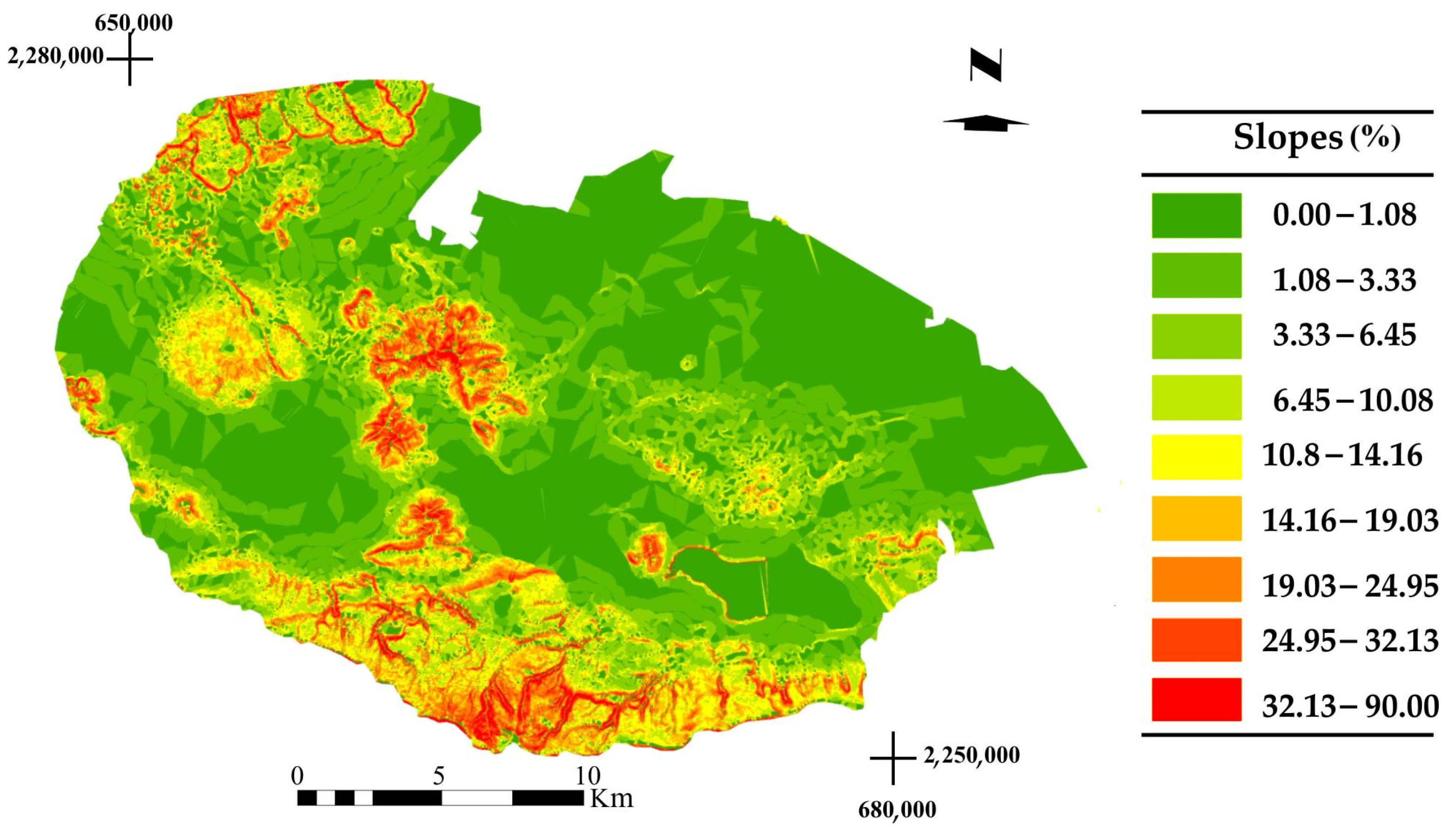
2.3. Determination of Environmental Covariables of the Soil-Forming Factors

To establish the covariables of the SCORPAN model [13], the covariables of the following factors were used: climate (C), organisms or vegetation (O), relief (R), and parent material (P); additionally, data on rock type, as well as some soil physical and chemical characteristics (S), were used. For factor C, Böhner & Antoniç [30] indicated that mean annual precipitation (PP) in millimeters (mm) and mean annual temperature (TEM) in °C are easily obtained variables; therefore, in our research, digital isohyet and isothermal maps of the municipality were used [24]. Additionally, Figueroa-Jáuregui et al. [31] mentioned that the use of vegetation indexes is useful for evaluation of the factor O. In the case of our study, we obtained the NDVI and the SAVI (soil-adjusted vegetation index) in the study area. These dimensional indexes were estimated by processing bands 4 (red) and 5 (near infrared) of a multispectral orthorectified Landsat 8 satellite image from 24 May 2020. The digital numbers of the different bands were transformed to reflectance levels to estimate NDVI and SAVI using Equations (1) and (2).

$$NDVI=\frac{\left(b5-b4\right)}{\left(b5+b4\right) }$$

(1)

where: NDVI is the normalized difference vegetation index; b4 is band 4 (red); and b5 is band 5 (near-infrared).

$$SAVI=\frac{\left(b5-b4\right)}{\left(b5+b4+L\right)}\ast \left(1+L\right)$$

(2)

where: SAVI is the soil-adjusted vegetation index; b4 and b5 are the same as in Equation (1); and L is a correction factor of soil luminosity [32] that, in our case, was 0.5. These estimations were carried out using ArcMap 10.3© software [33].

In the case of R, we used the slope [34], which was obtained from a digital elevation model (DEM) of the municipality [35] with a resolution of 15 m. Imperfections and vacant pixels were corrected using the FILL module of ArcMap 10.3©. Later, we obtained a digital map of slope percentages (SP) using the SLOPE module of the same software. Pike et al. [34] also pointed out that knowledge of the type of rock and its age is useful as a covariable of A. In our case, we used a digital map of the geology of the municipality of Tlajomulco, with which we obtained the distribution of geological material and its age (DAT) in millions of years [30].

To obtain the data of the different covariables for each sampling site of the thematic digital maps (TEM, PP, NDVI, SAVI, SP, DAT), we used the EXTRACTION module of ArcMap 10.3©, using the vector of points of the sampling sites.

In the case of S, the covariables that we used were the percentages of sand (SAN), silt (SILT), and clay (CLA) (as specific physical characteristics of the soils [S_p] under study) and the percentage of OM as the specific chemical characteristic of the soils (S_ch), which were obtained during the physical and chemical analyses of the soil samples.

Another factor considered was the human influence (HUM) exerted at each sampling site, measured as the amount of fertilizer in kilograms applied per hectare at each sampling site.

We generated a database of the data on pH (dependent variable) and the eleven covariables proposed (explanatory variables), together with the coordinates of each sampling point.

2.4. Descriptive Statistics and Multivariate Analysis

Using the database, we first obtained the descriptive statistics of the study variable and covariables, including the average, median, maximum and minimum values, typical deviation, asymmetry, and kurtosis.

Ranking of the covariables of the soil-forming factors that affect the behavior and distribution of the variable pH was achieved via a multivariate analysis using PCA in the software MINITAB 17 [36]. The principal components (PC) selected were only those that had an eigen value of more than one, according to the Kaiser Criterion, and that explained at least 70% of the accumulated variance [37]. In the same way, we considered the eigen vectors of each PC that had absolute values above 0.400.

2.5. Analysis of the Spatial Structure and Interpolation of the pH Data

The database was also used for the spatial structural study of pH, using semi-variance. According to Jaramillo [38], this type of study enables the determination of the existence of similarities among data at fixed distances (lag), using Equation (3).

$${\gamma }_{\left(h\right)}=\frac{1}{2N_{\left(h\right)}}{\sum }_{i=1}^{N_{\left(h\right)}}{[Z_{(X_i)}-Z_{\left(X_i+h\right)}]}^2$$

(3)

where: γ_(h) is the semi-variance for the pH of soils located in space at a given distance (h); N_(h) is the total number of pairs of data at a given distance (h); Z_(Xi) is the datum of the sample at a site Xi; and Z_(Xi+h) is the datum of the sample at a distance h from X.

The active distance in the study was 30,000 m, with asynchrony (lag) of 15 at sizes of 2.000 m for each lag. This experimental semi-variogram served as the basis for fitting the semi-variances to a spherical model and for quantifying pH spatial variability [21]. The parameters we used to explain this variability and obtain the prediction model were the nugget effect (Co), sill (Co + C), the structural variance (C), and the range [39]. In addition, we estimated the degree of spatial dependence [Co/(Co + C)] and the degree of spatial variation [C/(Co + C)] [38].

With the interpolator OK, we generated a predictive thematic map of pH (pH_p). According to Elbasiouny et al. [40], OK is useful for environmental and agricultural variables. The data were processed using ArcMap 10.3© [33], specifically with the extension Geostatistical Analyst. In the prediction maps, the results were grouped into four classes for pH_p. In the same extension, cross validation was performed to verify the accuracy of the predicted values derived from the prediction model (pH_p), with which the coefficient of determination (R²), the mean error of the prediction (ME_p), the root mean square error of the prediction (RMSE_p), the mean standard error of the prediction (MSE_p), the average standard error of the prediction (ASE_p), and the root mean square standardized error of the prediction (RMSSEp).

2.6. Verification of the pH Map

The accuracy of the pH_p prediction map was verified by digitally selecting 20 points in the prediction map. Simple random sampling was performed using the tool Create Random Points of the software ArcMap 10.3© to assure that the location of points was different from those used in the initial database. The UTM coordinates of each of the selected points were recorded. Later, each of the points was located in the field, where a simple sample of topsoil (0.30 cm deep) was collected. These samples were taken to the laboratory where they were prepared for their analysis, and pH was, again, determined. The results were compared with the values of the variable corresponding to each point of the prediction maps in an error matrix. The statistical indexes used to evaluate accuracy were the RMSE (root mean square error) and the MEB (mean error of the bias) using Equations (4) and (5) [41].

$$RMSE=\sqrt{\frac{{\sum }_1^n{\left(y-\hat{\mathrm{y}}\right)}^2}{n}}$$

(4)

where: RMSE is the root mean square error of the corresponding variable; y is the value of the variable estimated via the predictive model of the thematic pH_p map; ŷ is the value of the variable (pH), which was obtained from the soil samples at the points of verification; and n is the total number of samples.

$$MEB=\frac{{\sum }_1^n\left(y-\hat{\mathrm{y}}\right)}{n}$$

(5)

where: MEB is the mean error of the bias of the corresponding variable, and the remaining terms are the same as in Equation (4). The statistical program used at this stage was Minitab 17 [36].

3. Results

There were 101 sampled sites. The main crop was maize, and vegetables were grown at only one site. Soil management was mechanized, and the growers fertilized using urea (150 to 350 kg ha⁻¹).

The values of the covariables behaved differently within the study area. The texture classes identified were clay, clay loam, and sandy loam, with the occasional presence of gravel. Clay and loam textures were found in the lower parts, while sandy loams were found in the middle parts. Soil pH varied from 4.0 to 7.15 (

Table 1. Descriptive statistics of the environmental variables of the soil-forming factors.

Var	N †	$\stackrel{-}{\mathrm{X}}$	Σ	$\stackrel{-}{\mathrm{X}}$ ± σ	Min.	Median	Max.	Asy	Kur
pH	101	5.34	0.75	4.59–6.09	4.00	5.24	7.15	0.56	−0.51
OM	101	2.16	0.81	1.35–2.97	0.14	2.22	3.93	−0.31	0.14
CLA	101	66.67	10.37	56.30–77.04	40.00	69.50	82.00	−0.55	−0.61
SILT	101	16.40	5.12	11.28–21.52	7.00	16.00	32.00	0.35	−0.16
SAN	101	16.93	8.02	8.91–24.95	6.00	13.50	38.00	1.05	0.21
NDVI	101	0.22	0.082	0.14–0.30	0.04	0.22	0.68	2.04	11.07
SAVI	101	0.16	0.056	0.10–0.21	0.03	0.16	0.45	1.61	8.29
SP	101	11.66	10.17	1.49–21.83	0.17	5.55	80.59	2.51	6.16
TEM	101	19.50	0.78	18.74–20.28	14.90	19.70	20.30	−3.76	18.69
PP	101	839.40	33.32	806.08–872.72	742.00	830.00	919.00	0.38	−1.01
DAT	101	3.55	1.92	1.63–5.19	0.01	3.75	5.00	−1.16	−0.30
HUM	101	254.44	55.71	198.73–310.15	150.00	250.00	350.00	−0.20	−0.71

^† N: number of samples, $\stackrel{-}{\mathrm{X}}$: average, σ: standard deviation, Asy: asymmetry, Kur: kurtosis, OM: organic matter (%), SAN: sand (%), SILT: silt (%), CLA: clay (%), NDVI: normalized vegetation index, SAVI: soil-adjusted vegetation index, SP: slope percentage (%), TEM: temperature (°C), PP: precipitation (mm), DAT: age of dated geological material (millions of years), HUM: human influence (kg ha⁻¹).

), while the average value of OM was 2.16%. The average values of NDVI and SAVI (0.230 and 0.166, respectively) reflect the scarce plant cover; this was due to agriculture, since soil sampling was performed during the season of soil preparation.

Moreover, the soils were found on slopes of 11% on average (Figure 2). Nevertheless, the median (5.55%) indicates that half of the soils were found on flat land or gentle slopes (0–6%), while the other half were located on slopes, some of which were steep. The average temperature was 19.5 °C, while the average annual precipitation was 839.40 mm.

The asymmetry and kurtosis of most of the studied covariables are found within the interval of −3 to 3, although NDVI, SAVI, SP, and TEM had kurtosis above 3.

3.1. Multivariate Analysis of Environmental Covariables

The eigen values of the first five principal components are above one (

Table 2. Eigen values of the principal components.

	PC1	PC2	PC3	PC4	PC5	PC6	PC7	PC8	PC9	PC10	PC11
Eigen value	2.377	2.057	1.369	1.264	1.094	0.901	0.720	0.672	0.496	0.047	0.000
Proportion	0.216	0.187	0.124	0.115	0.099	0.082	0.065	0.061	0.045	0.004	0.000
Accumulated	0.216	0.403	0.528	0.643	0.742	0.824	0.889	0.951	0.996	1.000	1.000

), with an accumulated variance of 0.742; this means that, together, these components explain 74.2% of the variability of the pH.

These principal components (PC) have some eigen vectors with high absolute values (>0.400), which confirms the greater influence of the component (

Table 3. Eigen values of selected principal components.

Variable	PC1	PC2	PC3	PC4	PC5
OM	0.184	0.164	0.053	0.171	0.718
CLA	−0.624	−0.111	−0.094	−0.061	0.024
SILT	0.395	−0.129	0.247	0.183	0.112
SAN	0.555	−0.061	−0.037	−0.038	−0.102
NDVI	−0.071	−0.643	−0.209	0.167	0.075
SAVI	−0.091	−0.656	−0.163	0.105	0.113
SP	0.085	0.019	0.201	0.403	−0.589
TEM	0.168	0.178	−0.589	−0.171	0.107
PP	−0.249	0.009	0.455	0.300	0.234
DAT	0.028	−0.197	0.188	−0.656	−0.109
HUM	−0.029	0.158	−0.479	0.425	−0.132

).

PC1 is a function of the covariables clay (−0.624) and sand (0.555) (Table 3), indicating that high PC1 values correspond to sites with low clay content and high sand content. In contrast, low values of this component reflect high clay content and low quantities of sand. PC2 depends on NDVI (−0.643) and SAVI (−0.656), and when the two variables refer to plant cover, high values of this component reveal sites with little plant cover, while low values indicate sites with thick plant cover. In contrast, PC3 is related to temperature (−0.589), precipitation (0.455), and human influence (−0.479). High values of this component reflect sites with low temperatures and high precipitation, where the grower applies low quantities of fertilizer to the soil, while low values of this component indicate sites with high temperatures and low precipitation, where growers apply large quantities of fertilizer. PC4 depends on the age of the geological material (−0.656) and slope (0.403). High values of this component indicate sites with relatively recent geological material and steep slopes. In contrast, low values indicate older geological material and gentle slopes. Finally, PC5 is a function of OM (0.717), where high values of this component correspond to sites with higher OM content, and low values reveal soils with low percentages of OM.

Considering the above, the principal components that represent the factors, according to the SCORPAN model, are the following: PC1 is factor S (Sp), PC2 is factor O, PC3 is factor C and human influence, PC4 includes the factors A and R, and PC5 is, again, factor S but with Sch. This leads to the deduction that the spatial distribution of pH in the agricultural soils of Tlajomulco de Zúñiga would depend, first, on the covariables clay and sand, and second, on the covariable soil plant cover. In third place are the covariables precipitation and temperature and the covariable human influence. In fourth place are the covariables geological material and slope. Finally, in fifth place is the covariable OM.

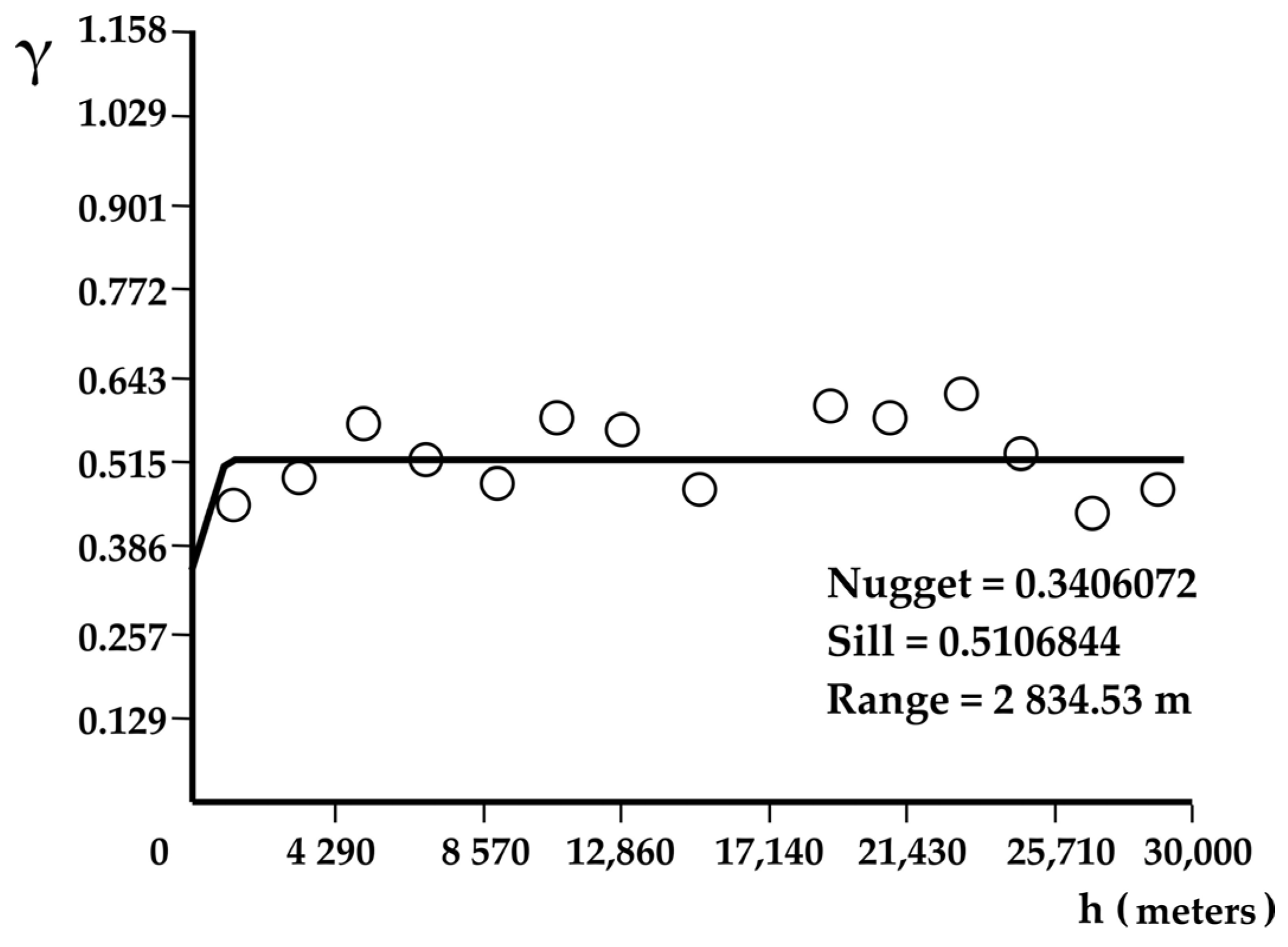
3.2. Analysis of the Spatial Structure of pH

The semi-variances (γ_(h)) of pH (Figure 3) were fit to a spherical model (R² = 0.6879), with a range equal to 2834.53 m, longer than the sampling distance (2500 m).

The nugget (0.3406) was lower than the sill (0.5106) but higher than the structural variance (0.1700), while pH spatial dependence (Co/(Co + C) = 66.7%) was moderate, according to the classification proposed by Cambardella [42], and the spatial variation (C/(Co + C)) was 33.3%. This was made evident through cross-validation, since the error (ME_p = 0.013 and MSE_p = 0.011) was small; the prediction map can thus be considered accurate. Moreover, when the uncertainty of the predictions was analyzed, it was found that the variability of the predictions was underestimated, since the RMSE_p of the pH_p (0.7781) was higher than the ASE_p (0.7429), as manifested with an RMSSE_p of more than one (1.0624).

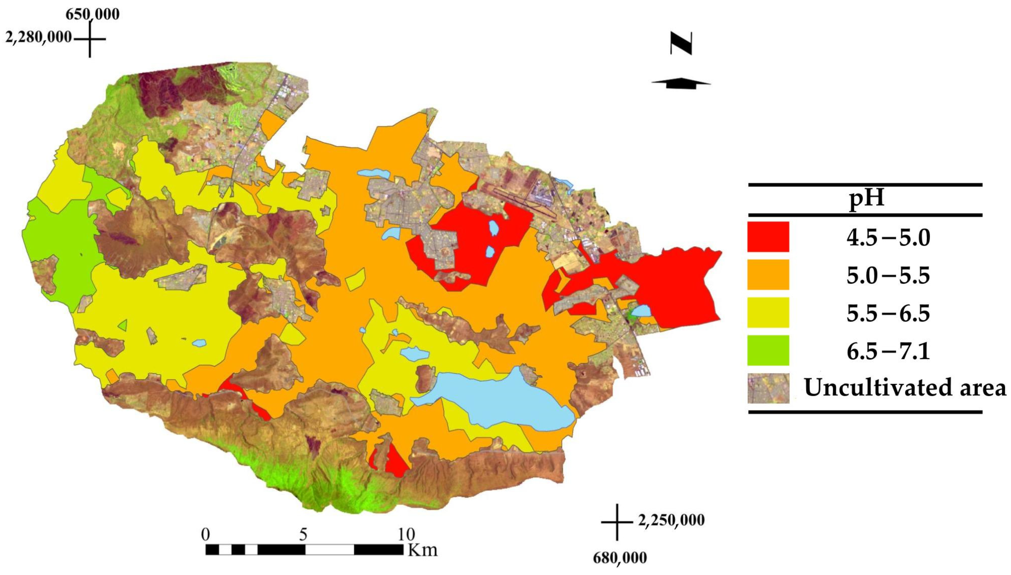
3.3. Spatial Distribution of pH

A pH class of 4.5–5.0 (strongly acid soil) is found mainly in the eastern portion of the farming area of Tlajomulco (Figure 4), occupying 14.2% of this area, while neutral soils (pH 6.5–7.1) are located in the western portion, covering 6.7% of the study area). Moderately acid soils occupy the rest of the area, and pH tends to decrease from west to east in the municipality.

3.4. Verification of the pH Map

The accuracy of the pH map was verified via cross-validation. Occasionally, it underestimated or overestimated the field value (

Table 4. Accuracy of the pH map of the municipality of Tlajomulco de Zúñiga, Jalisco.

N	UTM		† pHp	pHm	RMSE	MEB
	X	Y
1	664,920	2,271,661	5.1	5.0	0.01	0.10
2	676,133	2,266,878	4.8	4.9	0.01	−0.10
3	650,569	2,263,984	5.8	5.6	0.04	0.20
4	673,606	2,256,021	5.4	5.3	0.01	0.10
5	663,437	2,265,538	5.2	5.1	0.01	0.10
6	658,798	2,264,621	5.2	5.3	0.01	−0.10
7	672,989	2,271,684	4.1	4.0	0.01	0.10
8	662,276	2,262,246	5.2	5.2	0.00	0.00
9	661,783	2,275,120	5.1	5.4	0.09	−0.30
10	668,505	2,273,387	5.0	5.0	0.00	0.00
11	672,275	2,271,658	5.1	5.2	0.01	−0.10
12	651,688	2,270,674	6.1	6.2	0.01	−0.10
13	668,691	2,254,534	5.3	5.2	0.01	0.10
14	649,245	2,266,025	5.8	5.8	0.00	0.00
15	668,604	2,260,668	5.3	5.2	0.01	0.10
16	649,088	2,264,952	5.9	5.8	0.01	0.10
17	656,660	2,263,242	5.5	5.4	0.01	0.10
18	650,581	2,269,980	5.7	5.7	0.00	0.00
19	674,992	2,264,123	4.8	4.8	0.00	0.00
20	676,930	2,265,449	4.9	4.4	0.01	0.10
					0.158	0.020

^† pH_p: predicted pH; pH_m: field pH; RMSE: root mean square error of pH; MEB: mean error of the pH bias.

).

The RMSE value indicated that the map had good performance, since its result was close to zero (RMSE = 0.158). Nevertheless, the map had errors, as indicated by the bias of the predicted values relative to the observed values at each point. Thus, the MEB of the pH prediction map of our study showed a very low positive value (MEB = 0.020).

4. Discussion

4.1. Behavior of the Environmental Covariables

The values of the covariables each behave differently, reflecting their nature. The distribution of the texture classes of the soils in the study area correspond to existing reports for closed basins after sedimentation processes: the finest particles occupy the lowest areas, while the medium-sized particles are found in the middle part of the basin [43]. According to the interval of active acidity, the soils can be classified as extremely acid to neutral [6]; this is characteristic of the soils of the volcanic regions of Mexico and other parts of the world [44]. The percentages of OM are medium-to-low [29], corresponding to crop soils [43], such as those found in soils under traditional tillage [45]. When there is little or no vegetation, the NDVI and SAVI values are low [46]. Additionally, Ruiz-Corral et al. [47] reported that soils with gentle slopes occupy 62% of the agricultural area of the municipality of Tlajomulco. This is an important fact in terms of the conditions in which the soils are found, since slope influences soil’s physical and chemical properties [48], while temperature and precipitation correspond to regions with warm climates and dry springs and summers in the central part of the state of Jalisco [47] where Tlajomulco is found. Nevertheless, normal behavior of the data was demonstrated by asymmetry and kurtosis, found within the range of −3 to 3, which allows the assumption that 95% of the data of the variables fit a normal distribution. However, some variables had kurtosis above three, reflecting the values of variables at a distance greater than the normal distribution; this behavior is known as leptokurtic distribution, characterized by values that concentrate around the mean [49].

4.2. Effect of the Covariables on pH

Mineral particles that form part of the soil’s solid phase play an important role in pH behavior, since the reactions that occur between the solid phase components control pH. The clay fraction has a higher capacity to accept or donate protons than the acids or bases in the soil solution [18]. For example, when soil pH decreases, gradual hydrolysis occurs and the minerals release H⁺ ions, resulting in greater acidification [11]. Additionally, vegetation abundance and type also influence pH behavior [50]. This situation becomes evident in areas with annual crops during soil preparation, a stage at which there is little or no plant cover. Likewise, climatic elements such as precipitation and temperature changes also affect pH. On the one hand, water makes it possible for different reactions to occur among the components of the soil solid phase, and on the other, temperature accelerates or decelerates these reactions. For instance, in dry climates, these reactions cause a slow accumulation of cations, while in tropical climates, the reactions are accelerated and favor the percolation of cations [6]. Moreover, humans cause changes in the pH through fertilization of their crops [16]. When nitrogen fertilizers are added, microorganisms can oxidate NH₄⁺ to NO₃⁻, and thus, produce acidity [4]. The behavior of pH as a function of the covariables parent material and slope in our study coincides with the reports of Zhang et al. [12] and Ibarra-Castillo et al. [51]; they indicate that, depending on the mineralogical composition of the parent material, the results of their alteration will first be primary minerals, and later, during neogenesis, secondary minerals (crystalline or amorphous of clay size) [52,53], which modify pH, as mentioned previously. Slope, as a passive factor, influences the processes of parent material alteration, as well as the distribution and redistribution of the mineral particles in the soil during its formation, and these, in turn, affect pH [54]. Finally, OM affects pH, as Getachew et al. [11] indicate, since OM contains carboxyl and phenolic groups that can donate protons [4]; additionally, during the decomposition of these compounds, H⁺ ions, which are responsible for acidity, are released [11]. The above leads us to assume that the pH of the Tlajomulco soils is the result of constant interactions among the covariables of the soil-forming factors where soil acidification (the soil-forming process) would occur naturally and gradually. However, human activity, through the agricultural use of these soils, can accelerate the process by eliminating plant cover and applying nitrogen fertilizers for crop production, causing a decrease in pH. Nevertheless, when soil microbiology and mineralogy are unknown, it is not possible to specify the physical, chemical, or microbiological processes (pedogenetic processes) that occur in these soils. This information would be useful for soil management plans or for the recovery of soil with acidity problems [11,18].

4.3. Spatial Structure of pH

The spherical model obtained in this analysis is consistent with that reported in other studies that indicate that this model has a better fit with edaphic data (such as pH) in the definition of their spatial distribution [55]. Regarding the range, the result of our study is similar to that reported by Henríquez et al. [56], who obtained a range of 2480 m for pH. When the intervals or ranges are larger than the sampling distances, a spatial relationship among the samples is revealed that suggests strong autocorrelation, possibly due to some factor that has a greater influence than the sampling distance [57]. We are thus dealing with a characteristic that has less variability and maintains its autocorrelation at greater distances [56]. This coincides with the results of our research, in which the characteristics specific to soil, such as the content of clay and sand, and environmental factors, such as climate, plant cover, topography, and the distribution of geological material and its age, influence the distribution of pH. In this sense, when a nugget smaller than the sill is found, the structure and spatial dependence are manifested [58]. Additionally, moderate spatial dependence correlates with some environmental and soil characteristic [59]. In this way, the results of the analysis of pH spatial structure indicate that pH is spatially predictable and has a low level of uncertainty when interpolated [38,56]. This was confirmed in our study via cross-validation. According to ESRI [33], when the value of MSE is close to zero, the level of uncertainty is low, while a value of RMSSE greater than one indicates underestimation of the prediction variability. This situation was found in our results (MSE = 0.011 and RMSSE = 1.0624), indicating that the predictive pH map could underestimate pH values, but would be accurate because of the low error.

4.4. Spatial Distribution of pH

The distribution of pH classes on the map could be related to the way the soil was formed and to the human use of this resource. In general, the locations of the pH classes on the map are related to the environmental covariables that are analyzed in our study. Soils with a pH between 4.5 and 5.0 have clay textures (with pumice gravel) and are used for agriculture, with applications of up to 350 kg of urea. These are sites where the geological material is volcanic pyroclastic, 2.5 to 5.0 million years old [24], on flat land (Figure 2), and with a low content of OM. In contrast, soils with a pH between 6.5 and 7.1 have a clay loam texture and are used for agriculture with applications of 150 kg urea; they are a geological material of stable alluvion composed of fine particles of volcanic origin and are found on gentle slopes. According to Acevedo-Sandoval et al. [8], soil acidification can occur during pedogenesis as the result of the interrelationship of different factors and soil-forming processes, considering human influence as the catalyst of these processes. In this sense, the alteration of OM is slower in soils with a pH below 5.0 [15]. This phenomenon in our study is likely associated with agricultural use of these soils, since the maize monocrop is fertilized with urea (up to 350 kg ha⁻¹) during every crop cycle. This behavior was reported by Cruz-Macías et al. [17], who associated the decrease in pH with the application of ammonium fertilizers. Likewise, Zang et al. [60] indicated that the addition of nitrogen fertilizers decelerates OM alteration due to the decrease in microbial activity. It is probable that a study of soil genesis that includes soil microbiology and mineralogy, to establish the processes resulting from the interactions among soil-forming factors, would help explain pH behavior with greater precision and contribute to proposing management and recovery plans for acid soils with longer-lasting effects.

4.5. Precision of the pH Map

RMSE values equal to zero indicate a perfect fit of the data given by the simulation or prediction model to the observed data [61]. Additionally, the statistical test MEB can express overestimation or underestimation of the simulation or predictive models. These cases are denoted by their sign, whether positive or negative [41]. The above means that the pH thematic map underestimated the field values. Under these criteria, in our study, the thematic map of pH prediction is accurate, as estimated by the analysis of the spatial structure of the data and verified via cross-validation. Therefore, the map could serve as a basis for locating soils with acidity problems in decision-making for the management of these soils; however, more research is required that evaluates the pH map of the Tlajomulco de Zúñiga soils, for management purposes.

5. Conclusions

The methodology used in this research allowed us to stablish the environmental covariables of the soil-forming factors that affect the distribution and spatial variability of pH, which were defined and ranked. In addition, a map of this edaphic variable was obtained. The environmental covariables that represented the soil-forming factors explained 74.2% of pH spatial variability in the soils of Tlajomulco. In order of importance, from most to least important, the covariables that were grouped as a function of soil-forming factors were as follows: the physical characteristics of the soil, the vegetation, the climate, the age of the parent material together with the factor relief, and finally, the chemical characteristics of the soil (S_p > O > C > A-R > S_ch). Moreover, human activity influences soil pH through the application of nitrogen fertilizers. The analysis of the spatial structure of pH demonstrated that this variable had moderate spatial dependence (66.7%) and was thus spatially predictable. The predictive thematic map of soil pH was accurate (RMSE = 0.158 and MEB = 0.020) in placing the pH classes in the municipality of Tlajomulco de Zúñiga, Jalisco. This methodology could serve as the basis for formulating proposals for the management and recovery of soils with acidity problems. However, more research is needed; it is also necessary to include soil microbiological and mineralogical variables in these types of studies to understand processes that could occur when applying amendments to improve soil quality so that the effect is longer-lasting.

References

1. Pahlavan-Rad, M.R.; Akbarimoghaddam, A. Spatial variability of soil texture fractions and pH in a flood plain (case study from eastern Iran). Catena 2018, 160, 275–281. [Google Scholar] [CrossRef]
2. Saleh, A.M. Spatial Variability Mapping of Some Soil Properties in Jadwal Al_Amir Project/Babylon/Iraq. J. Indian Soc. Remote Sens. 2018, 46, 1481–1495. [Google Scholar] [CrossRef] [Green Version]
3. Zhu, H.; Hu, W.; Bi, R.; Peak, D.; Si, B. Scale-and location-specific relationships between soil available micronutrients and environmental factors in the Fen River basin on the Chinese Loess Plateau. Catena 2016, 147, 764–772. [Google Scholar] [CrossRef]
4. Bloom, P.R.; Skyllberg, U. Soil pH and pH Buffering. In Handbook of Soil Science, 2nd ed.; Huang, P.M., Li, Y., Sumner, M.E., Eds.; Volume 1: Properties and processes; CRC Press (Taylor & Francis): Boca Raton, FL, USA, 2012; pp. 19.1–19.14. [Google Scholar]
5. Tu, C.; He, T.; Lu, X.; Luo, Y.; Smith, P. Extent to which pH and topographic factors control soil organic carbon level in dry farming cropland soils of the mountainous region of Southwest China. Catena 2018, 163, 204–209. [Google Scholar] [CrossRef]
6. Weil, R.R.; Brady, N.C. The Nature and Properties of Soils, 15th ed.; Pearson Education Limited: London, UK, 2017; 1104p. [Google Scholar]
7. Lo Monaco, P.A.V.; Júnior, G.R.; Vieira, G.H.S.; Meneghelli, C.M.; Simon, C.P. Conchas de ostras e cascas de ovos moídas como corretivos da acidez do solo. Eng. Agric. 2016, 25, 584–590. [Google Scholar] [CrossRef]
8. Acevedo-Sandoval, O.; Valera-Pérez, M.A.; Prieto-García, F. Propiedades físicas, químicas y mineralógicas de suelos forestales en Acaxochitlan, Hidalgo, México. Univ. Cienc. 2010, 26, 137–150. [Google Scholar]
9. Hernández-Jiménez, A.; Llanes-Hernández, V.; Terry-Alfonso, E.; Carnero-Lazo, G. pH changes in brown soils of Cuba when eroded. Cult. Trop. 2020, 41, e04. [Google Scholar]
10. Shiferaw, T.; Tadele, M. Review on Effect of Soil Acidity on Barley (Hordeum vulgare L.). J. Nat. Sci. Res. 2022, 13, 13–17. [Google Scholar]
11. Getachew, A.; Chilot, Y.; Teklu, E. Soil Acidity Management; Ethiopian Institute of Agricultural Research (EIAR): Addis Ababa, Ethiopia, 2019; 56p. [Google Scholar]
12. Zhang, Y.-Y.; Wu, W.; Liu, H. Factors affecting variations of soil pH in different horizons in hilly regions. PLoS ONE 2019, 14, e0218563. [Google Scholar] [CrossRef] [Green Version]
13. McBratney, A.B.; Mendonca-Santos, M.L.; Minasny, B. On digital soil mapping. Geoderma 2003, 117, 3–52. [Google Scholar] [CrossRef]
14. Zhao, W.; Li, J.; Jianga, J.; Lua, H.; Honga, Z.; Qiana, W.; Xua, R.; Denga, K.; Guana, P. The mechanisms underlying the reduction in aluminum toxicity and improvements in the yield of sweet potato (Ipomoea batatas L.) after organic and inorganic amendment of an acidic ultisol. Agric. Ecosyst. Environ. 2020, 288, 106716. [Google Scholar] [CrossRef]
15. Sellan, G.; Thomson, J.; Majalap, N.; Robert, R.; Brearley, F.Q. Impact of soil nitrogen availability and pH on tropical heath forest organic matter decomposition and decomposer activity. Pedobiologia J. Soil Ecol. 2020, 80, 150645. [Google Scholar] [CrossRef]
16. Fageria, N.K.; Nascente, A.S. Management of soil acidity of South American soils for sustainable crop production. Adv. Agron. 2014, 128, 221–275. [Google Scholar]
17. Cruz-Macías, W.O.; Rodríguez-Larramendi, L.A.; Salas-Marina, M.A.; Hernández-García, V.; Campos-Saldaña, R.A.; Chávez-Hernández, M.H.; Gordillo-Curiel, A. Efecto de la materia orgánica y la capacidad de intercambio catiónico en la acidez de suelos cultivados con maíz en dos regiones de Chiapas, México. Terra Latinoam. 2020, 38, 475–480. [Google Scholar] [CrossRef]
18. Kome, G.K.; Enang, R.K.; Tabi, F.O.; Yerima, B.P.K. Influence of Clay Minerals on Some Soil Fertility Attributes: A Review. Open J. Soil Sci. 2019, 9, 155–188. [Google Scholar] [CrossRef] [Green Version]
19. Djodjic, F.; Bieroza, M.; Bergström, L. Land use, geology and soil properties control nutrient concentrations in headwater streams. Sci. Total Environ. 2021, 772, 145108. [Google Scholar] [CrossRef]
20. Alemán-Montes, B.; Búcaro-González, A.; Henríquez-Henríquez, C.; Largaespada-Zelaya, K. Mapeo digital de suelos agrícolas en la región occidental del Valle Central de Costa Rica. Agron. Costarricense 2019, 43, 157–166. [Google Scholar] [CrossRef]
21. Yescas-Coronado, P.; Álvarez-Reyna, V.P.; Segura-Castruita, M.A.; García-Carrillo, M.; Hernández-Hernández, V.; González-Cervantes, G. Variabilidad Espacial del Carbono Orgánico e Inorgánico del Suelo en la Comarca Lagunera, México. Bol. Soc. Geol. Mex. 2018, 70, 591–610. [Google Scholar] [CrossRef]
22. Malone, B.; Minasny, B.; McBratney, A. Using R for Digital Soil Mapping; Springer: Cham, Switzerland, 2017; 262p. [Google Scholar]
23. Colín García, G.; Fernández-Reynoso, D.S.; Martínez-Menez, M.R.; Ríos-Berber, J.D.; Sánchez-Guzmán, P.; Rubio-Granados, E.; Ibáñez-Castillo, L.A. Clasificación digital de suelos a través de covariables ambientales de la cuenca del río Mixteco. Terra Latinoam. 2017, 35, 281–291. [Google Scholar]
24. Gobierno del Estado de Jalisco. Actualización del Atlas Municipal de Riesgos por Amenazas Naturales y Antrópicas en el Municipio de Tlajomulco de Zúñiga, Jalisco. Mapa Geológico. 2018. Available online: https://tlajomulco.gob.mx/ProteccionCivil/1.1.7%20MAPA%20GEOL%C3%93GICO.pdf (accessed on 20 December 2020).
25. García, E. Modificaciones al Sistema de Clasificación Climática de Köppen; Instituto de Geografía-Universidad Nacional Autónoma de México: México city, Mexico, 2004; 98p. [Google Scholar]
26. SMN (Servicio Meteorológico Nacional). Normales Climatológicas Periodos 1951–2010 y 1981–2000. Servicio Meteorológico Nacional, México, 2015. Available online: http://smn.cna.gob.mx (accessed on 20 December 2020).
27. IIEG-Jalisco (Instituto de Información Estadística y Geografía de Jalisco). Recursos Cartográficos/Suelos, Vegetación y Uso del Suelo. 2018. Available online: https://iieg.gob.mx/contenido/Municipios/TlajomulcodeZuniga.pdf (accessed on 18 December 2020).
28. INEGI (Instituto Nacional de Estadística y Geografía). Sistema de Descarga de Productos Digitales. 2019. Available online: http://www.beta.inegi.org.mx/temas/mapas/topografico/ (accessed on 5 December 2020).
29. NOM-021-RECNAT-2000S; Norma Oficial Mexicana que establece las Especificaciones de Fertilidad, Salinidad y Clasificación de Suelos. Estudios, Muestreos y Análisis. Diario Oficial de la Federación: México, Mexico, 2002; 85p.
30. Böhner, J.; Antoniç, O. Land-Surface parameters specific to topo-climatology. In Geomorphometry. Concepts, Software, Applications; Hengl, T., Reuter, H., Eds.; Elsevier: Amsterdam, The Netherlands, 2009; pp. 195–213. [Google Scholar]
31. Figueroa-Jáuregui, M.L.; Martínez-Menez, M.R.; Ortiz-Solorio, C.A.; Fernández-Reynoso, D. Influencia de los factores formadores en las propiedades de los suelos en la Mixteca, Oaxaca, México. Terra Latinoam. 2018, 36, 287–299. [Google Scholar] [CrossRef]
32. Vani, V.; Mandla, V.R. Comparative study of NDVI and SAVI vegetation indices in Anantapur district semi-arid areas. Int. J. Civ. Eng. Technol. 2017, 8, 559–566. [Google Scholar]
33. ESRI (Environmental Systems Research Institute). ArcGis 10.3. Recorrido Rápido por la ArcGIS Spatial Analyst Extension. 2014. Available online: https://desktop.arcgis.com/es/arcmap/10.3/guide-books/extensions/spatial-analyst/a-quick-tour-of-spatial-analyst.htm (accessed on 18 January 2020).
34. Pike, R.J.; Evans, I.S.; Hengl, T. Geomorphometry: A brief Guide. Dev. Soil Sci. 2009, 33, 3–30. [Google Scholar]
35. INEGI (Instituto Nacional de Estadística y Geografía). Continuo de Elevaciones Mexicano. INEGI. Aguascalientes, México. 2015. Available online: http://www.inegi.org.mx/ (accessed on 5 December 2020).
36. Minitab Inc. Minitab® State College. Minitab Inc. Pennsylvania, EEUU. 2013. Available online: https://www.minitab.com/es-mx/ (accessed on 15 August 2021).
37. Cuadras, C.M. Nuevos Métodos de Análisis Multivariante; CMC: Barcelona, Spain, 2020; 304p. [Google Scholar]
38. Jaramillo, D.F. Variabilidad espacial del suelo, bases para su estudio. Rev. Fac. Cienc. 2012, 1, 73–87. [Google Scholar]
39. Gallardo, A. Geostadística. Ecosistemas 2006, 15, 48–58. [Google Scholar]
40. Elbasiouny, H.; Abowaly, M.; Alkheirb, A.A.; Gad, A.A. Spatial variation of soil carbon and nitrogen pools by using ordinary Kriging method in an area of north Nile Delta, Egypt. Catena 2014, 113, 70–78. [Google Scholar] [CrossRef]
41. Douglas, E.M.; Jacobs, J.M.; Sumner, D.M.; Ray, R.L. A comparison of models for estimating potential evapotranspiration for Florida land cover types. J. Hydrol. 2009, 373, 366–376. [Google Scholar] [CrossRef]
42. Cambardella, C.A.; Moorman, T.B.; Parking, T.B.; Karlen, D.L.; Novak, J.M.; Turco, R.F.; Konopka, A.E. Field-scale variability of soil properties in central Iowa soils. Soil Sci. Soc. Am. J. 1994, 58, 1501–1511. [Google Scholar] [CrossRef]
43. López-Acevedo, R.M.; Poch, C.R.M.; Porta, C.J. Edafología: Uso y Protección de Suelos; Cuarta, Ed.; Mundi-Prensa Libro: México city, Mexico, 2019; 624p. [Google Scholar]
44. Zúñiga, F.; Buenaño, M.; Risco, D. Caracterización física y química de suelos de origen volcánico con actividad agrícola, próximos al volcán Tungurahua. Rev. Ecuat. Investig. Agropecu. 2016, 1, 5–10. [Google Scholar] [CrossRef] [Green Version]
45. Mishra, U.; Ussiri, D.A.; Lal, R. Tillage effects on soil organic carbon storage and dynamics in Corn Belt of Ohio USA. Soil Till. Res. 2010, 107, 88–96. [Google Scholar] [CrossRef]
46. Torres, E.; Linares, G.; Tenorio, M.G.; Peña, R.; Castelán, R.; Rodríguez, A. Índices de vegetación y Uso de Suelo en la Región Terrestre Prioritaria 105: Cuetzalan, México. Rev. Iberoam. Cienc. 2014, 1, 112–120. [Google Scholar]
47. Ruiz-Corral, J.A.; Valdez-Díaz, L.E.; Flores-López, H.E.; Medina-García, G.; Ramírez- Díaz, J.L.; Pérez-Domínguez, J.F.; Aceves-Rodríguez, J.J.; González-Ávila, A.; Soltero-Díaz, L.; Medina-Ocegueda, S.; et al. Potencial productivo agrícola de la región centro de Jalisco; Centro de Investigación Regional del Pacifico Centro, INIFAP: México city, Mexico, 2005; 84p. [Google Scholar]
48. Wang, Y.; Zhang, X.C.; Zhang, J.L.; Li, S.J. 2009. Spatial variability of soil organic carbon in a watershed on the loess plateau. Pedosphere 2009, 19, 486–495. [Google Scholar] [CrossRef]
49. Camacho, R.; Salazar, S.; González, L.; Pacheco, H.; Suárez, C. Caracterización geomorfológica de las dunas longitudinales del Istmo de Médanos, estado Falcón, Venezuela. Investig. Geográf. 2011, 76, 7–19. [Google Scholar] [CrossRef]
50. Panico, S.C.; Ceccherini, M.T.; Memoli, V.; Maisto, G.; Pietramellara, G.; Barile, R.; De Marco, A. Effects of different vegetation types on burnt soil properties and microbial communities. Int. J. Wildland Fire. 2020, 29, 628–636. [Google Scholar] [CrossRef]
51. Ibarra-Castillo, D.; Ruiz-Corral, J.A.; González-Eguiarte, D.R.; Flores-Garnica, J.G.; Díaz-Padilla, G. Distribución espacial del ph de los suelos agrícolas de Zapopan, Jalisco, México. Agric. Téc. Méx. 2009, 35, 267–276. [Google Scholar]
52. Wilson, M. Weathering of the primary rock-forming minerals: Processes, products and rates. Clay Minerals 2004, 39, 233–266. [Google Scholar] [CrossRef] [Green Version]
53. Churchman, G.J.; Lowe, D.J. Alteration, formation and occurrence of minerals in soils. In Handbook of Soli Science, 2nd ed.; Huang, P.M., Li, Y., Sumner, M.E., Eds.; Volume 1: Properties and processes; CRC Press (Taylor & Francis): Boca Raton, FL, USA, 2012; pp. 20.1–20.72. [Google Scholar]
54. Sidari, M.; Ronzello, G.; Vecchio, G.; Muscolo, A. Influence of slope aspects on soil chemical and biochemical properties in a Pinus laricio forest ecosystem of Aspromonte (Southern Italy). Eur. J. Soil Biol. 2008, 44, 364–372. [Google Scholar] [CrossRef]
55. Sreenivas, K.; Dadhwal, K.V.; Kumar, S.; Harsha, G.S.; Mitran, T.; Sujatha, G.; Janaki, G.R.S.; Fyzee, M.A.; Ravisankar, T. Digital mapping of soil organic and inorganic carbon status in India. Geoderma 2016, 269, 160–173. [Google Scholar] [CrossRef]
56. Henríquez, C.; Méndez, J.C.; Masís, R. Interpolación de variables de fertilidad de suelo mediante el análisis kriging y su validación. Agron. Costarric. 2013, 37, 71–82. [Google Scholar] [CrossRef]
57. Villatoro, M.; Henríquez, C.; Sancho, F. Comparación de los interpoladores IDW y Kriging en la variación espacial de pH, Ca, CICE y P del suelo. Agron. Costarric. 2008, 32, 95–105. [Google Scholar]
58. Yamamoto, J.K.; Landim, P.M.B. Geoestatística: Conceitos e Aplicações; Oficina de Textos: São Paulo, Brazil, 2013; 215p. [Google Scholar]
59. Pingguo, Y.; Byrne, J.M.; Yang, M. Spatial variability of soil magnetic susceptibility, organic carbon and total nitrogen from farmland in northern China. Catena 2016, 145, 92–98. [Google Scholar] [CrossRef]
60. Zang, H.; Wang, J.; Kuzyakova, Y. N fertilization decreases soil organic matter decomposition in the rhizosphere. Appl. Soil Ecol. 2016, 108, 47–53. [Google Scholar] [CrossRef]
61. Soto-Bravo, F.; González-Lutz, M.I. Análisis de métodos estadísticos para evaluar el desempeño de modelos de simulación en cultivos hortícolas. Agron. Mesoam. 2018, 30, 517–534. [Google Scholar] [CrossRef]
Figure 1. Location of the study area in Jalisco, México.
Agriculture 12 02132 g001
Figure 2. Slopes of the soils of the municipality of Tlajomulco de Zúñiga, Jalisco.
Agriculture 12 02132 g002
Figure 3. Semi-variogram of active acidity (pH).
Agriculture 12 02132 g003
Figure 4. Thematic pH map of the municipality of Tlajomulco de Zúñiga, Jalisco.
Agriculture 12 02132 g004