SCMC: An Efficient Scheme for Minimizing Energy in WSNs Using a Set Cover Approach

Abstract

Energy-efficient clustering and routing are well known optimization problems in the study of Wireless Sensor Network (WSN) lifetime extension. In this paper, we propose an intelligent hybrid optimization algorithm based on a Set Cover approach to create clusters, and min-cost max-flow for routing (SCMC) to increase the lifetime of WSNs. In our method we used linear programming (LP) to model the WSN optimization problem. This model considers minimizing the energy for all nodes in each set cover (cluster), and then minimizing the routing energy between the nodes and the base station through intermediate nodes, namely cluster heads. To evaluate the performance of our scheme, extensive simulations were conducted with different scenarios. The results show that the set cover approach combined with the min-cost max-flow algorithm reduces energy consumption and increases the network’s lifetime and throughput.

1. Introduction

The term “Wireless Sensor Network” (WSN) refers to a large number of spatially distributed autonomous nodes that organize themselves into a multi-hop wireless network for the monitoring and recording of physical or environmental conditions. Their applications include battlefield surveillance, target tracking, security, environmental control, habitat monitoring, source localization, fire detection, oil and gas pumping, and many more.

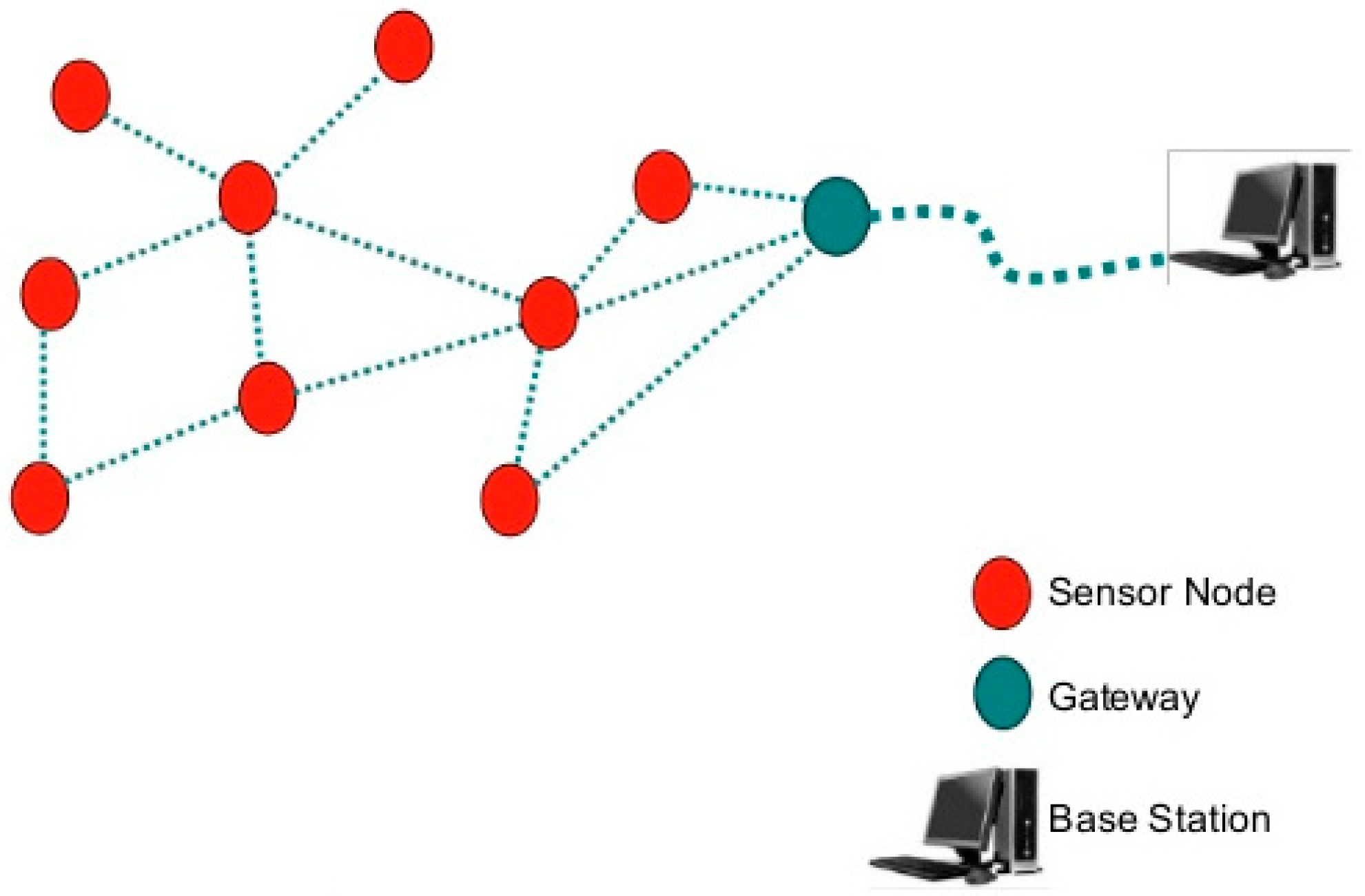
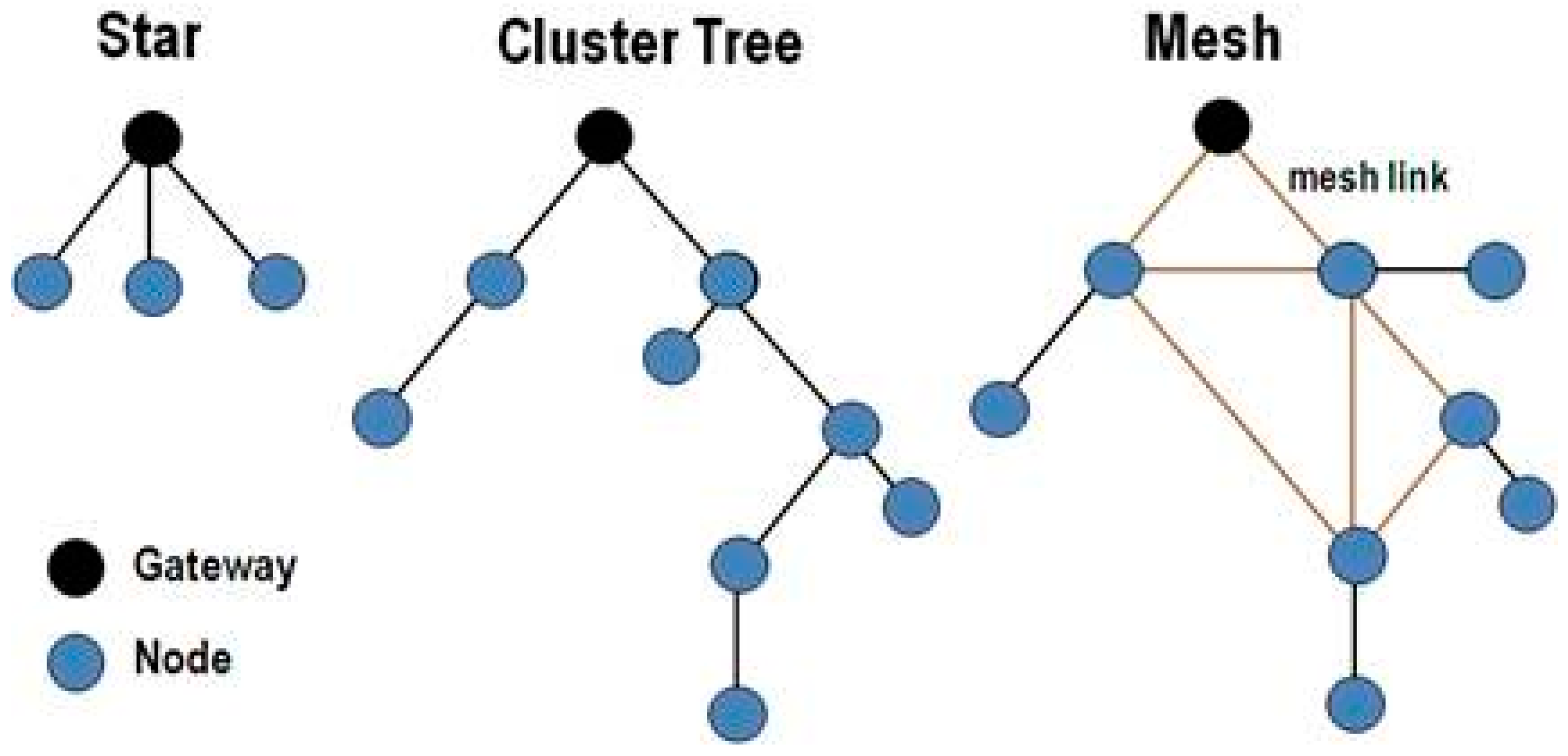
A WSN system consists of distributed nodes and a gateway that provides wireless connectivity back to the wired world (see Figure 1). They can be organized into three types of network topology as shown in Figure 2.

Figure 1. Wireless Sensor Network (WSN) Components, Gateway, and Distributed Nodes.

Figure 2. WSN Topologies.

A star network topology consists of a single base station and multiple remote nodes. The nodes cannot communicate directly with each other, while the base station can communicate with all of the nodes. In a mesh network topology, a node can directly communicate with any other node within its transmission range. This solves the single point of failure problem of star networks by allowing what is called multi-hop communication. In a cluster network topology, nodes are grouped to form a cluster with one of the nodes elected as a “cluster head” (CH). Cluster topologies when employed in WSNs generally result in lower energy consumption and an increased overall lifetime of the network.

Because they are usually deployed in harsh environmental scenarios, WSN nodes rely solely on their batteries most of the time. As batteries have a finite capacity, minimizing energy consumption in order to extend the lifetime of sensor nodes without compromising their functionality is an important area of study in WSN research [1,2,3,4,5].

In WSNs, all nodes usually share common sensing tasks, each covering a different target area. This implies that not all sensors that are deployed within the same target area are required to perform their task continuously throughout the system’s entire lifetime. Sensor nodes consume more energy when they are in transmission mode (active) than when they are in sleeping mode (inactive). If all sensor nodes within a coverage target area are active, the data collected will be redundant and a large amount of energy will be consumed and wasted. To save the overall energy of WSNs, our approach was to activate some sensor nodes while turning off others within each target area (set cover/cluster) without losing or disrupting system connectivity.

Specifically, the proposed model aims to determine a minimum set cover within a WSN, and to elect a relay node (cluster head) that will forward sensor node messages to the base station. Moreover, the model addresses the problem of finding the minimum cost routes from sensor nodes to the base station through the elected cluster heads using a min-cost flow algorithm. To achieve the best solution for expanding a WSN’s lifetime, we propose a modified version of the min-cost flow algorithm by taking residual energy as a constraint value to judge different paths and choose the best one among them, i.e., the one with the highest residual energy.

While most of the approaches found in literature employ a Particle Swarm Optimization (PSO) algorithm to find clusters [6,7,8,9,10], in this paper we present a novel approach based on a set cover algorithm for finding clusters and a min-cost max-flow algorithm to find paths with minimum cost (energy consumption) and maximum residual energy. There are two main motivations for finding minimum set covers and using min-cost max-flow routing. The first is the need for an efficient energy scheme in WSNs, where sensor nodes tend to use small batteries for energy supply, and which are in many cases non-replenishable. Therefore an efficient activation management scheme is needed to conserve their energy, and thus that of the whole network. The second is the need for reliability in wireless networks. This need stems from the unpredictable nature of the wireless environment, which unlike its wired counterpart is more prone to link failures due to dead sensor nodes. A typical scenario where our approach can be of particular interest is if we consider a monitoring application targeted at the structural integrity of buildings, with WSN nodes deployed for data collection purposes over key city constructions such as roads, buildings, and bridges. When one critical event is detected (e.g., a dangerous flexure of a column), the monitoring application should trigger an alert to be delivered immediately to the WSN’s data collection points (base station). In this case, it is particularly important to increase resiliency against link failures and ensure a long lifetime, which is what the SCMC technique presented in this paper achieves.

The remainder of the paper is organized as follows: Section 2 presents related work, Section 3 presents the approach, Section 4 describes simulation results, and Section 5 concludes the paper.

2. Related Works

Three key considerations in WSNs are coverage [11], connectivity [12], and battery lifetime [13]. Coverage refers to how well an area is monitored, while connectivity means that each node or device should be connected such that the data is sent back to the base station (BS). Any applied heuristic needs to fulfill the requirement of Q-coverage and P-connectivity, where Q is the minimum number of sensors monitoring any one point in the area, and P is the number of disjoint paths between any two sensors.

In this section, we shall take a brief tour of the past approaches at solving these issues, starting with [14] in which the authors proposed a heuristic method called QC-MCSC to maximize the network lifetime while satisfying both the coverage and connectivity requirements. This method consists of three phases or layers where the output of one phase is the input of the next one. The first phase is the Coverage phase, which outputs the set of sensors that cover all the target areas. Next is the Connectivity and Redundancy Reduction phase, which takes the set of the first phase and applies the Breadth-First Search (BFS) algorithm to find the shortest path for each sensor. In this phase, unnecessary nodes are removed and any extra nodes are only added if the network is not fully connected, and the output is a minimal connected set cover of nodes. Finally, the Energy and Priority Updating phase determines the lifetime constant of each set cover from the second phase. The lifetime constant is the minimum lifetime available from sensors in a set cover. In this phase, if the battery life ‘B’ of one node is less than the energy needed for communicating and sensing ‘E’, the node is removed from the set cover. Through simulation, the authors compared the Q-Coverage Maximum Connected Set Cover (QC-MCSC) algorithm with the Three Phase Iteration Connected Set Cover (TPICSC) algorithm [15] and the results showed that the former achieves a higher lifetime. Furthermore, the results of the simulations reveal that the proposed heuristic (QC-MCSC) is very close to the actual optimal result.

A difficulty that researchers face when they want to expand the coverage time span is the question of how to distribute the sensors into separate independent subdivisions, known as Disjoint Set Covers (DSC). This problem is identified as having an NP-hard complexity, and many researches have used the Boolean sensing model to solve it.

To facilitate topic lookup for the reader, we shall broadly divide the remaining studies by the type of approach and/or the specific WSN issue being addressed.

2.1. Target Coverage

A number of studies have focused on addressing the target coverage problem. The objective of the authors in [16] for example, was to have the maximum number of targets monitored by sensor nodes before they run out of energy. To extend the network lifetime, they proposed an approach to calculate the maximum number of disjoint sensor covers with a heuristic greedy algorithm using three parameters: (1) the set covers; (2) the number of targets; (3) the number of sensors. The proposed approach finds the set covers that can be used to maximize the network lifetime of a WSN in polynomial time. They showed that it gives a local maximum solution due to its heuristic search.

Maintaining full connectivity of the WSN was the primary focus of [17], in which the authors proposed an algorithm for ensuring that both conditions (i.e., coverage and connectivity) are met for conserving energy and extending the lifetime of the WSN. It relies on a distributed response procedure to locate the routes between the sensors and the sinks. The procedure allows for several routes leading from a sink to individual sensors to be discovered. Depending on the set of routes, a Minimum Distance Path (MDP) greedy algorithm is derived from resolving the Maximum Set Cover (MSC) issue with the goal of locating the highest possible number of set covers. The MDP-MSC algorithm works with the concept of choosing the sensors possessing the shortest distance to the set cover under construction, in order to include them into the contemporary set cover after each process. In this algorithm, the discovered routes, which are determined by the maximum number of routes per cover, influence the choice of sensors that are added to the set cover. The authors stated that the optimum value of the maximum number of routes per cover, as well as the level of density of the sensors within the target area, all impact the performance and control of transmission overhead in the WSN.

Based on simulation and experimental analysis using MDP-MSC, a number of set covers received a noticeable growth by 13% and 21% compared to the Greedy-MSC [18] and Heuristic Approach-Multidimensional Scaling (HA-MDS) algorithms [19]. MDP-MSC did not just outperform Greedy-MSC and HA-MDS; it also had the lowest time complexity between them. MDP-MSC achieved a balanced consumption of energy and less computational time.

On the other hand, the authors in [20] proposed a distributed lifetime coverage optimization (DiLCO) protocol to preserve coverage as well as boost the WSN’s lifetime. The protocol begins by applying a divide and conquer algorithm to split the target location into smaller regions known as sub-locations, after which it is concurrently carried out in every single sub-location. Assumptions are made that the partitioning of the sub-locations is carried out in a regular manner and that the sensors are set uniformly in each sub-location. The periodic DiLCO protocol possesses four stages in each period: information exchange, leader election, decision, and sensing. Every period possesses a single set cover handling the sensing operation. This type of cyclic scheduling boosts the reliability of the WSN against sensor failures. Sensors without sufficient power to successfully carry out a period or those that fail before the decision phase is completed are not included in the scheduling procedure. If a sensor fails after being chosen, the quality is only reduced for the duration of the period as another functioning sensor is selected in the next period.

Two types of packets were used when carrying out the DiLCO protocol: info and Active/Sleep. Info packets are transmitted from a sensor to all others within the same sub-location with the purpose of providing information. Active/Sleep packets are transmitted by the leader to the other sensors within the same sub-location to notify them to set their status to either Active or Sleep in the sensing stage.

The challenges faced in implementing the DiLCO protocol lie in selecting the most appropriate leader in every single sub-location and the most suitable collection of active sensors to ascertain a high standard in coverage.

In [21], the aim was to find the maximum number of sensor coverage sets. The authors used two centralized algorithms and one localized algorithm. The two centralized algorithms deal with how the sensors are added to make a connected cover. The localized algorithm is used for communication between the local nodes. All three algorithms were only run once during the initialization phase. They concluded that keeping one coverage set active in a round-robin fashion would extensively reduce the energy consumption.

2.2. Node Activation

With regards to node activation, many existing studies propose alternating nodes between Sleep and Active modes, or regulating the sensing range of the nodes. The authors in [22] however, proposed to use both approaches together by setting up the minimum sensing radius for each sensor in the Active state. This reduces the active node’s density, thereby reducing useless Media Access Control (MAC) layer interference, which would otherwise consume lots of power.

2.3. Node Distribution

The authors in [23] proposed to choose the smallest possible number of nodes that will cover the critical targets by using a cost function called the Critical Control Factor. This function is mapped into 3 loops: (1) sensor availability check (adding the cover sets); (2) uncovered target check (populating the added cover sets with sensors); and (3) sensor applicability check (sorting the nodes and choosing the top-scoring node). The main benefits of this proposed solution are that it is flexible, has a low complexity, and has a short execution time. In the end, the authors concluded that there are two solutions for node deployment: static and dynamic. In the static method, the proposed algorithm performed better than the other approaches in terms of execution time, and exhibited near-optimal results in the generated coverage sets. The dynamic method on the other hand yielded better results but with a longer execution time.

2.4. Redundancy Management

Redundancy plays an important role in maintaining the reliability of a WSN by handling unforeseen failures and boosting the accuracy of calculated computations, due to the infeasibility of replacing the failed sensors. Due to this infeasibility, prolonging the network lifetime to ensure that measurements are taken for as long as possible is another desired trait. The Location-Unaware Coverage (LUC) algorithm [24] addresses the issue of finding a balance between efficient redundancy and network lifetime. The LUC algorithm determines whether a sensory node will be actively receiving measurements or sleeping to preserve its energy. To carry this out, each sensor node determines its neighbors and their relative distance in a two-hop neighborhood. LUC carries out a series of geometric and heuristic tests to determine the ‘strength’ of the nodes, with the weaker ones put to sleep initially. The stronger nodes possess a higher reliability, and hence are kept active for a longer duration. The LUC algorithm has two protocols: Iterative LUC (LUC-I) and Probabilistic LUC (LUC-P), which determine whether nodes will be set in Active or Sleep mode through a series of hops. The protocols bring about low operating costs and may greatly minimize the number of nodes that are active.

Upon completion of the protocols, all nodes are set to either the Sleep or the Active mode. Active nodes are responsible for covering the entire target area, and the WSN’s lifetime and reliability are both improved.

2.5. Clustering

The authors in [25] proposed to use the Low-Energy Adaptive Clustering Hierarchy (LEACH) protocol [26] with the Fuzzy Inference System (FIS) based on Mamdani’s method [27] to select cluster heads and to extend the lifetime of WSNs. FIS consists of a fuzzifier, an inference engine, and a defuzzifier. The proposed model uses three parameters: distance to coordinator, energy, and density. IF-THEN rules are used to calculate the chance for a sensor node to become a cluster head. The chance value is obtained by defuzzification, which aggregates the results of each rule. Then, the node chooses the maximum of the chance values and compares it to a pre-defined threshold value. If it is found to be less than the threshold then it becomes the cluster head. Experimental studies conducted with LEACH and LEACH-Fuzzy Logic (LEACH-FL) showed that using LEACH-FL increased the network’s lifetime twice more than when using LEACH.

2.6. Set Cover

A greedy set cover algorithm was proposed by the authors in [28]. It selects the minimum number of sensors that are disseminated into disjoint and non-disjoint sets, with the necessity that every set cover completely fulfills the scope of all its targets. They stated that the proposed algorithm is an improvement over the classical greedy set cover algorithm, and its approximation ratio is verified to be not worse than log(m). Through simulations, they demonstrated that their algorithm performed better than others from previous research efforts.

2.7. Optimization

Finally, many authors have considered the distribution of sensors and energy optimization as a multi-objective optimization problem. The authors in [29] for instance proposed an Efficient Cover Set Selection (ECSS) approach, which is an improved version of the Non-Dominated Sorting Genetic Algorithm (NSGA-II) [30]. The goal of the proposed scheme is to maintain full coverage by using fewer sensors. They highlighted that having more active sensors results in more coverage but with a lower overall lifetime, and vice versa.

The authors concluded that the ECSS algorithm had advantages such as the ability to reset all the sensors’ statuses with a one-time approach. It could also be made flexible by providing it with parameters such as the requested field coverage and the model.

In another approach named the Multi-Objective Set Cover Problem (MO-SCP) [31], the authors considered reliable coverage as an additional conflicting objective to be optimized. They tried to solve it using a multi-objective evolutionary algorithm to select the set with the minimum number of sensor nodes, such that it will provide coverage of all the targets. To meet the requirement of staying active for long periods, the authors proposed to alternate nodes between idle and active states through something called ‘wake-up scheduling’ of the sensors. Their objective was to achieve a WSN system which can actively sense its predefined targets almost all the time. With the implementation of this method, only a single disjoint set is active while the others are kept in sleep mode (in a specific interval), resulting in an energy conservation scheme. When the active set goes out of power, another set is scheduled to be in the active state. Therefore with this approach, the more DSCs that there are the better it is for the entire system to stay on power. Moreover, they adopted a heuristic crossover operator designed specifically to improve the performance of the algorithm, and conducted simulation scenarios to test the effectiveness of the proposed algorithm.

In this paper, we propose an approach that combines a set cover method with a min-cost max-flow algorithm using a linear programming technique.

3. Approach

The proposed algorithm passes through three main phases: (1) information gathering; (2) set cover formation; and (3) path determination.

During the information-gathering phase, all of the sensor nodes including the base station are assigned a unique ID. They then broadcast their IDs using the Carrier-Sense Multiple Access with Collision Avoidance (CSMA/CA) MAC layer protocol, which allows the base station to discover sensor node locations. Now, with the help of the received information about the network, the base station starts the creation of set covers, electing cluster heads and determining optimal routing paths using network layer information. It is to note that once the set cover creation and path determination phases are over, all cluster heads are aware of the next hop to the base station and sensor nodes are also informed about the cluster head ID that they belong to. Then, each cluster head provides a TDMA schedule to its member sensor nodes for intra-cluster communication.

We modeled the energy conservation problem as an optimization problem where a “single objective function” is used for the minimum set covers, and for the min-cost max-flow model too. Our key contribution is that the proposed model guarantees a longer network lifetime.

3.1. Network Model and Assumptions

A wireless sensor network is composed of a set of battery-powered sensors and a sink. The latter is connected to a power source and so we disregard its energy consumption in this paper. Communication between the sensors is achieved through wireless links if they are within range of each other, or through other intermediate sensors if not.

Thus, a WSN can be modeled as a unit disk graph [32,33] G = (V, E) where V is the set of all nodes including the sink and E ∈ V × V is a set of possible communication links. We assume our graph is connected.

S = {s₁, s₂, ..., s_N} represents a collection of N sensor nodes that are distributed randomly in a two-dimensional plane to monitor a set of target nodes T = {t₁, t₂, ...., t_M}.

Given two nodes s₁ and s₂ (one of them should be a sensor), they are connected by an edge (s₁, s₂) ∈ E, if the first sensor is within the sensing coverage range of the second sensor. Thus, two nodes s₁ and s₂ can communicate with each other (there is an edge between them) if ||d(s₁, s₂)|| ≤ 1, where ||d(s₁, s₂)|| is the Euclidean distance between s₁ and s₂.

Each sensor node s_i ∈ S, can operate into a number of sensing ranges r₁, r₂, ..., r_p where each r_k consumes energy e_k, 1 ≤ k ≤ P. The initial energy of each sensor node is E. A sensing node s_i ∈ S can cover a target t_i ∈ T using sensing range r_k if the Euclidean distance d(s_i, t_j) is less than or equal to r_k, denoted as t_j → s_i. Then, we define the target subset T_i = {t_j | t_j → s_i, 1 ≤ j ≤ m} as the target set of the sensor s_i.

We assume that at regular time intervals, the information sensed by a network node has a fixed unit size of b bits that can be stored at the sensor in a buffer of infinite capacity, modeled as a First In First Out (FIFO) queue. We also assume that the channel bandwidth for all links is W bps and that all transmitted packets have a unit size of b bits. Only one packet can be transmitted in each time slot t, which is defined as t = b/W seconds. Time-division multiple access (TDMA) is used at the MAC layer.

3.2. Cluster Creation

Our main purpose is to extend the network lifetime as much as possible, and to minimize the energy consumption by keeping the amount of traffic to a minimum and by scheduling nodes to monitor a set of targets continuously in turn. To facilitate the achievement of our objective, a set of clusters is constructed. Many studies have adopted the creation of clusters in WSNs [34,35,36], however only some of them considered the use of a set cover algorithm. In this study, we consider the construction of a minimum set cover C = {Ci}, 1 ≤ i ≤ K to create clusters. The problem can be described formally as follows.

Set Cover Definition and Creation

The set cover problem is one of Karp’s 21 NP-complete problems shown to be NP-complete in 1972 [37].

The set cover optimization has many applications in different areas [38] including manufacturing, service planning, location problems, network security, and multiple sequence alignments for computational biochemistry [39,40,41,42].

Given a set of elements (called the universe) and a collection S of m sets whose union equals the universe, the set cover problem is to identify the smallest sub-collection of S whose union equals the universe.

In our paper we adopt the following approach: using a greedy set cover algorithm [19] to choose which cover a sensor node will belong to. In this approach, we define a finite set S = {S₁, S₂, S₃, …, S_m}, corresponding to the areas to be monitored, a collection {S_j}n_j = 1 of subsets of S, where each S_j represents a sensor and contains the areas that the sensor monitors from S, and a positive integer k ≥ 2. The goal is to find a partition G of the subsets into k covers c₁, ..., c_k where each cover is a set of subsets, such that N(G) = k_i=1 |∪ S_j ∈ c_i S_j| is minimized.

The heuristic used in our paper consists of greedily picking sets from S. The set S_j ∈ S that contains the most number of uncovered vertices is picked at each step. We repeat the process until all vertices are covered. The following is the pseudo-code of the greedy set cover algorithm.

Greedy Set Cover Algorithm

U$\leftarrow X$ // U is the set of uncovered elements S’$\leftarrow \varnothing$ // S’ is the current set cover While U$\ne \varnothing$ Do    Pick Sj $\in S$ such that |Sj ${{\displaystyle \cap }}^{\text{}}U$| is maximized    S’$\leftarrow$S’${{\displaystyle \cup }}^{\text{}}$ Sj    U$\leftarrow$U−Sj end

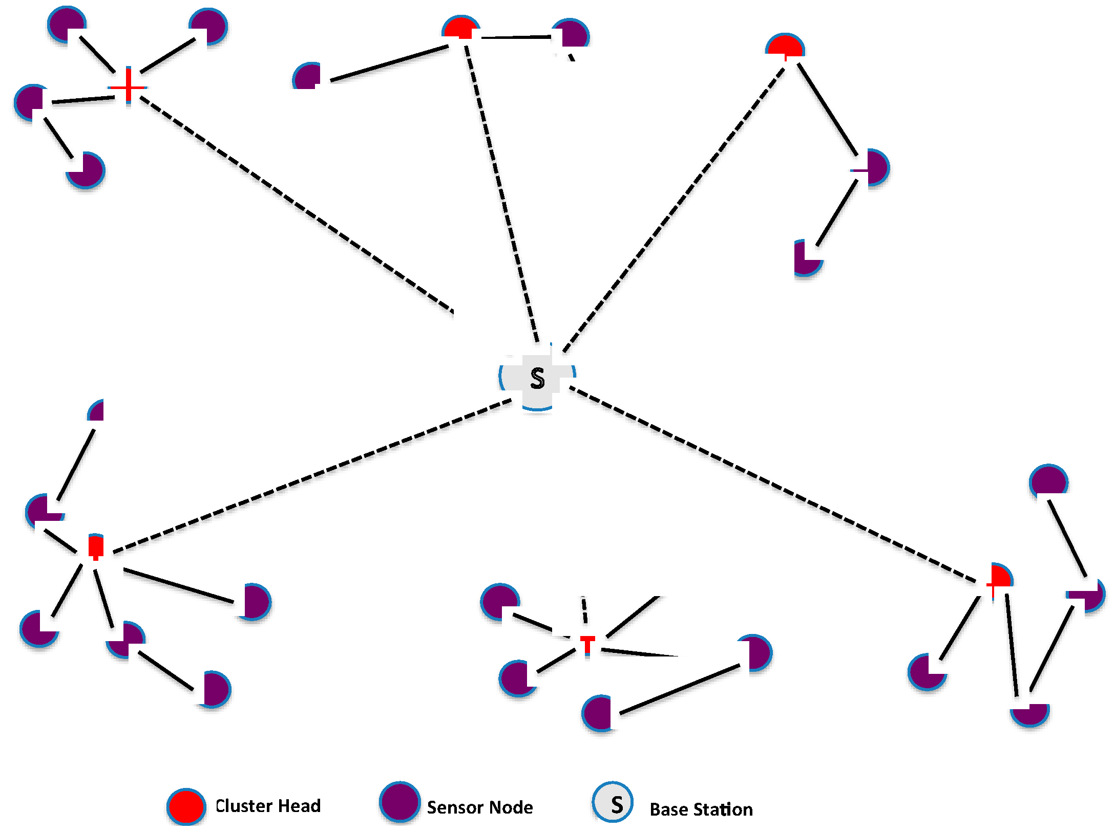
Once the set covers (clusters) are constructed, some sensor nodes become cluster heads (CHs) and collect all traffic from their respective cluster. The cluster head aggregates the collected data and then sends it to the base station as shown in Figure 3. The CH is chosen based on the highest residual energy, thus allowing the network lifetime to increase in proportion to node density [43].

Figure 3. Cluster creation with cluster head elected.

When using clustering, the workload on the cluster head is thus larger than for non-cluster heads. To maximize the lifetime of cluster heads, we propose to elect two cluster heads within each cluster that have the highest energy, and interchange their roles in a round-robin fashion during their lifetime in order to distribute and balance the extra workload and energy consumption evenly between them.

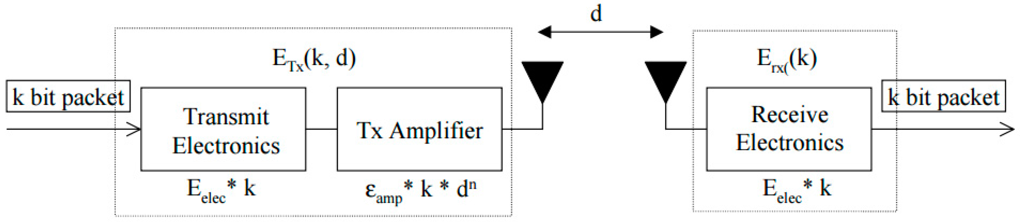
3.3. Energy Consumption Model

The energy consumption model adopted in this paper is based on the proposed model in [44] which has been used by many researchers [45,46,47,48,49,50]. In this model, it is assumed that the transmitter, power amplifier, and receiver all dissipate energy to run the radio electronics as shown in Figure 4.

Figure 4. Radio Energy Dissipation Model.

The power attenuation is dependent on the distance between the transmitter and the receiver. For relatively short distances, the propagation loss can be modeled as inversely proportional to d², whereas for longer distances the propagation loss can be modeled as inversely proportional to d⁴. Power control can be used to invert this loss by setting the power amplifier to ensure a certain power at the receiver. Thus, to calculate the transmission cost (joule/bit) and the receiving cost (joule/bit) for a message of size k bits from a sensor node i (transmitter: T_x) to a sensor node j (receiver: R_x) over a distance d(i,j) (Euclidian-Distance), where the energy consumption at node i comprises operating radio electronics and amplifiers while at node j only radio electronics, the following equations are used:

Transmission cost:

E_TX(k, d) = k × E_TX-elec + E_TX-amp(k, d) = k × E_TX-elec + k × d² × E_amp,

(1)

Receiving cost:

E_RX(k, d) = k × E_RX-elec,

(2)

where E_elec is the energy dissipation of the radio in order to run the transmitter and receiver circuitry, and E_amp is the transmitter amplifier.

Typical values used in this paper during the simulation are:

E_elec = 50 nJ/bit, E_amp = 100 pJ/bit/m², d² = 500, and the packet size k = 2000 bits [49].

If we consider that node i wants to transmit an amount of data f_ij to node j, the energy consumption (Joules) at node i will be:

$$E_{TX,I}={{\displaystyle \sum }}_{\begin{array}{c}j=1\\ i\ne j\end{array}}^n\left(E_{TX,ij}\ast f_{ij}\right)$$

(3)

On the other hand, if node j wants to send an amount of data f_ji to node i, the energy consumption (Joules) at node i will be:

$$E_{RX,I}=E_{RX}{{\displaystyle \sum }}_{\begin{array}{c}j=1\\ i\ne j\end{array}}^n{f}_{ji}$$

(4)

Thus, the total energy consumed at node i will be:

E_consu,i = E_TX,i + E_RX,I

(5)

3.4. Energy Optimization

Once the clusters are created, our objective is to minimize the energy consumption when routing data to the base station. First, we minimize energy consumption within each cluster, and then we minimize the routing energy consumption.

3.4.1. Minimizing Energy Consumption in Clusters

The objective of using a SET K-COVER approach to construct clusters in WSNs is to increase their energy efficiency. The reason for the common placement of multiple sensors close together to cover a single area is due to the ad-hoc nature of sensor placement, topological constraints, or to compensate for the short lifetime of the sensors.

Therefore, in an effort to increase the longevity of the network and to conserve battery power, it is beneficial to activate groups of sensors in rounds, so that the battery life of a sensor is not wasted on areas that are already monitored by other sensors. Additionally, certain batteries last up to twice as long when used in short bursts as opposed to continuously. Therefore, activating a sensor only once every k time units can extend the lifetime of its battery. For the active nodes inside a cluster, an energy cost e_i is associated with a sensor node x_i each time the latter sends a message to the CH.

Thus, the energy consumption for a cluster can be formulated as a linear programming optimization problem where:

$$\mathrm{Minimizing}{{\displaystyle \sum }}_{i=1}^k{x}_i\ast e_i,$$

(6)

where k is the number of active nodes inside the cluster.

St:

$$e_i\le E_{init}$$

(7)

$$x_i=\{\begin{array}{ll}1& ifactive\\ 0& ifinactive\end{array}$$

(8)

$${{\displaystyle \sum }}_1^k{e}_i\le E_{clust}$$

(9)

where E_init is the initial energy of node x_i, where E_clust is the initial cluster total energy of all nodes.

Output: vector X = (x₁, x₂, …x_n) for nodes active and inactive.

3.4.2. Routing Energy Optimization

It is to note that in order to achieve the effective collection of data, WSNs must meet two requirements. One is full coverage of the targets, and the other is complete connectivity of the network. Full coverage means that the sensors should be able to monitor all targets, and complete connectivity means that the data that originated from the monitoring targets should be able to reach the base station through multi-hop wireless communication using a minimum energy path.

We believe that relying only on a minimum energy routing strategy has some deficiency in terms of network lifetime. Since most of the time using a relay node is more energy-efficient than direct communication with the base station, sensor nodes closer to the base station exhaust their batteries long before other nodes residing on the perimeter of the network area. Hence, network lifetime cannot be optimized with minimum energy routing alone. As a solution, we propose to take into consideration the residual energy of the nodes in the path by assigning link costs inversely proportional to the residual energy values. This way, energy consumption could be balanced throughout the whole network. In fact, such a solution can achieve maximal network lifetime using a linear programming (LP) based model.

Network Model

After clustering, the routing procedure is invoked during data transmission using a min-cost max-flow algorithm [51].

The Wireless Sensor Network used in this paper is modeled as a directed graph G (V, E), where V represents the set of sensor nodes and E the set of edges.

Each edge (u, v) ∈ E is associated with a cost c (u,v) which represents the energy consumption when there is a flow f_ij going out from u to v, a capacity constraint u_ij expressed in the number of packets per unit time, and a supplies/demands variable d_ij. The cost of a flow is: f (u,v). c (u,v).

The objective is to deliver all the data generated by the sensor nodes to the base station with minimum energy consumption and without exceeding the link capacities.

The problem can be formulated as follows:

Minimizing the total cost of the flow over all edges:

$${\displaystyle \sum }_{\left(u,v\right)\in E}f\left(u,v\right).c\left(u,v\right)$$

(10)

St:

$$f\left(u,v\right)\le c\left(u,v\right)\forall \left(u,v\right)\in E$$

(11)

$$f\left(u,v\right)=-f\left(v,u\right)$$

(12)

$${{\displaystyle \sum }}_{w\in V}f\left(u,v\right)=0forallu\ne s,t$$

(13)

$${{\displaystyle \sum }}_{w\in V}f\left(v,w\right)-{{\displaystyle \sum }}_{w\in V}f\left(w,v\right)=d$$

(14)

where (11) represents the capacity constraint, (12) the skew symmetry, (13) the flow conservation, and (14) the required flow.

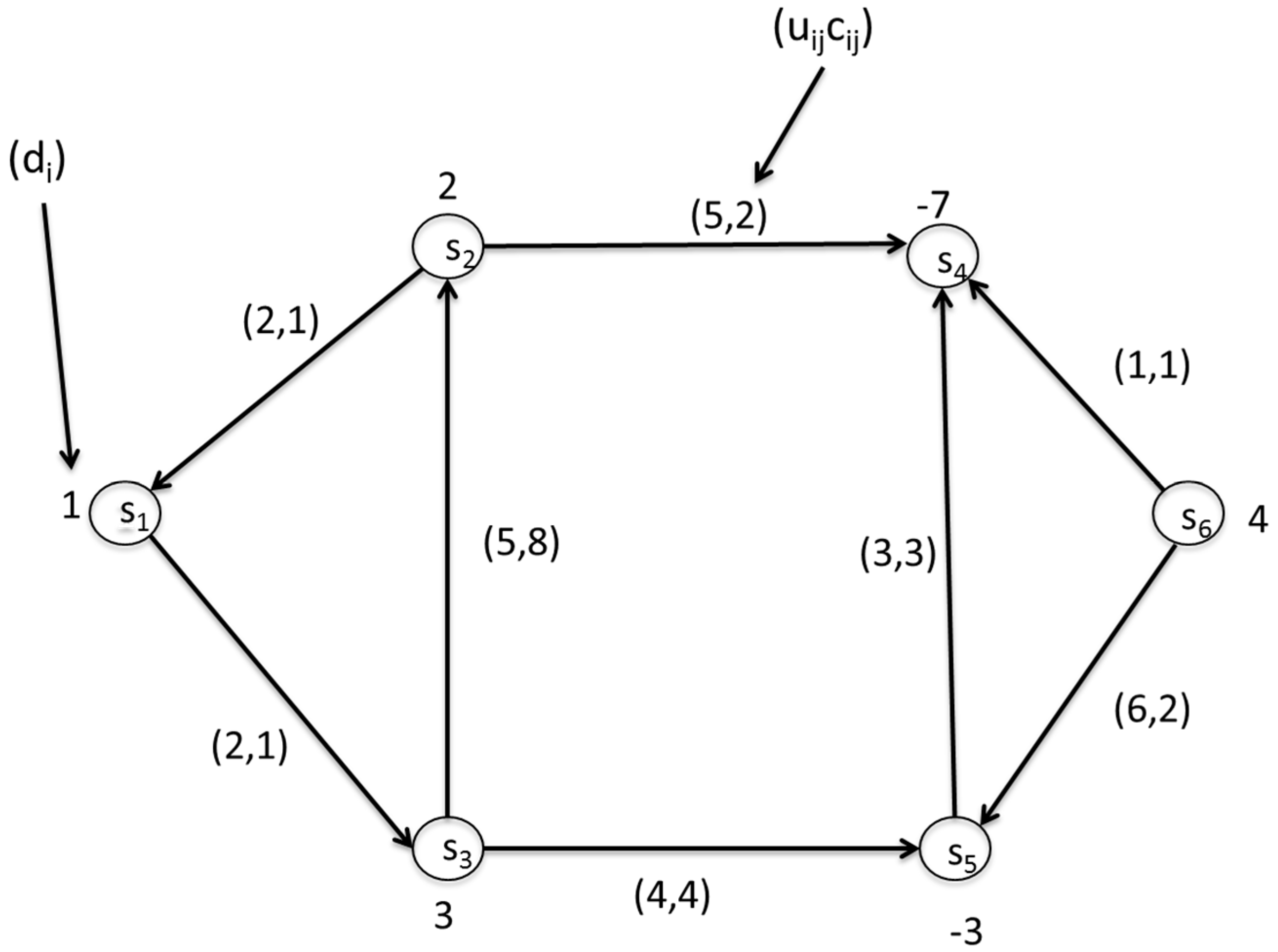
The above problem can be converted into a minimum-cost circulation problem [52] and can be solved efficiently using well-known min-cost flow algorithms [53,54,55,56]. In this research we adopt a network simplex method [57] as it is considered the most practical algorithm [57]. Figure 5 shows a sample of a sensor network where s₁ is the source and s₆ is the destination. The flow capacities and demands are shown on the graph.

Figure 5. WSN graph representation.

The corresponding network simplex LP is as follows, where x_ij = Number of units shipped from node i to j using arc i–j:

Min z = x₁₃ + 2x₂₁ + 2x₂₄ + 8x₃₂ + 4x₃₅ + 3x₅₄ + x₆₄ + 2x₆₅

Node s₁: x₁₃ − x₂₁ = 1

Node s₂: x₂₁ + x₂₄ − x₃₂ = 2

Node s₃: −x₁₃ + x₃₂ + x₃₅ = 3

Node s₄: −x₂₄ − x₅₄ − x₆₄ = −7

Node s₅: −x₃₅ + x₅₄ − x₆₅ = −3

Node s₆: x₆₄ + x₆₅ = 4

x₁₃ ≤ 2x₂₁ ≤ 2x₂₄ ≤ 5x₃₂ ≤ 5x₃₅ ≤ 4x₅₄ ≤ 3x₆₄ ≤ 1x₆₅ ≤ 6

4. Simulation Results

In order to assess our model, we compared it to the MO-SCP, MDP-MSC, and LEACH models.

We performed a set of simulation scenarios in MATLAB [58] using a variable number of sensor nodes (100, 200, 300, 400) deployed randomly in a 1500 m² area. This allowed us to evaluate the effectiveness of our proposed approach and analyze its impact on the energy of the entire network, and thus on the lifetime of the WSN. Parameters used in the simulation are similar to those used in [59], and are shown in Table 1.

Table 1. Simulation parameters.

Parameters	Value
Initial energy Einit	0.5 J
Transmitting and receiving energy Eelec	5 nJ/bit
Amplification energy for short distance Ef	10 Pj/bit/m2
Amplification energy for long distance Eamp	0.013 pJ/bit/m4
Packet size	200 bits
Operating frequency	2.4 GHz
Initial energy of sensor	61,560 J
Transmit power	32 mW
Reference distance	3 m
Path loss exponent	4
Signal to Noise Ratio	2 dB

Our experiment consists of two phases of WSN network design: cluster set cover creation and path determination.

In both phases, we input the set of SNs, their locations, the required network lifetime, and other parameters to the corresponding SCMC model. We then solved the WSN design model with the IBM^® ILOG^® OPL-CPLEX^® optimization solver.

In the first phase the set cover model is used to obtain the optimal number of set covers with their corresponding CH, and the optimal packet transmission path from SNs to the selected CH inside each cluster. In the second phase we use the results obtained from the first phase to derive the optimal path between the CH and the BS using the min-cost max-flow algorithm. The metrics used to test the effectiveness of our proposed approach are based on the percentage of Alive nodes, the round where the First Node Dies (FND), the round where the Last Node Dies (LND), and the network throughput.

The results of the first phase are shown in Table 2. The Greedy algorithm creates a number of set covers for each scenario where the number of sensor nodes is varied (N = 100, 200, 300 and 400)

Table 2. Set covers number created by Greedy algorithm.

Number of Nodes	Number of Clusters
100	7
200	8
300	7
400	8

In the second phase, the min-cost max-flow model is solved as stated before and a comparison is carried out between the different approaches on the basis of the metrics stated earlier. Table 3 and Table 4 summarize the results of these metrics.

Table 3. Number of rounds when 10%, 20%, 30%, 40%, 50%, 60%, 70% and 80% of nodes die.

Protocol	Percentage of Alive Nodes
	90	80	70	60	50	40	30	20
LEACH	1100	1642	1600	1465	2278	2500	2986	2987
MDP-MSC	1600	1855	1900	1978	2436	2875	3100	3300
MO-SCP	1756	1860	2150	2360	2780	3164	3600	3785
SCMC	1865	1890	2260	2600	2830	3700	4300	4500

Table 4. Nodes die-off statistics of the different approaches.

Protocol	FND	LND
LEACH	1019	1986
MDP-MSC	1125	3125
MO-SCP	1019	4035
SCMC	975	9800

Table 3 shows the number of rounds completed by various schemes when 10%, 20%, 30%, 40%, 50%, 60%, 70% and 80% of nodes die for N = 100.

It is evident, as shown in Table 3, that SCMC has a better performance than its counterpart protocols. For instance, in the case of SCMC the number of rounds when 80% of nodes are dead is 4500 whereas in the case of MO-SCP, MDP-MSC, and LEACH the number is 3785, 3300, and 2987 respectively. Therefore, SCMC extends the lifetime of the WSN and can provide information for a considerably longer period of time. This lifetime increases with node density, where SCMC takes the advantage of the set cover formation and the optimal routing energy.

Despite the fact that SCMC has its first node dead in an earlier round than the other approaches, it shows very promising results, with the death of all nodes as shown in Table 4 occurring at about 9800 rounds compared to 4035 for MO-SCP, 3125 for MDP-MSC, and 1986 for LEACH. Furthermore, we clearly see that when 20% of nodes at the same number of rounds in SCMC are alive, all nodes in the other approaches are dead.

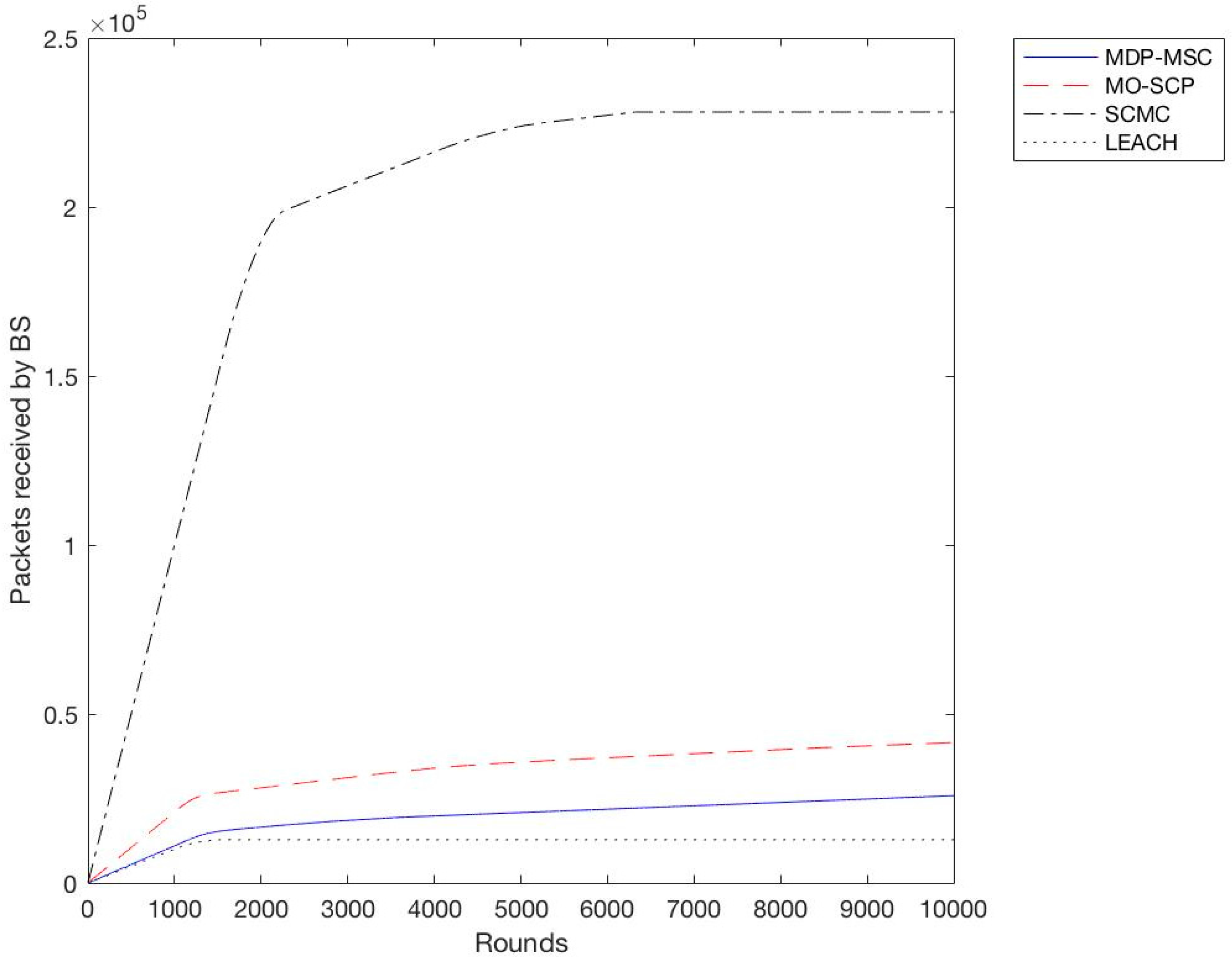
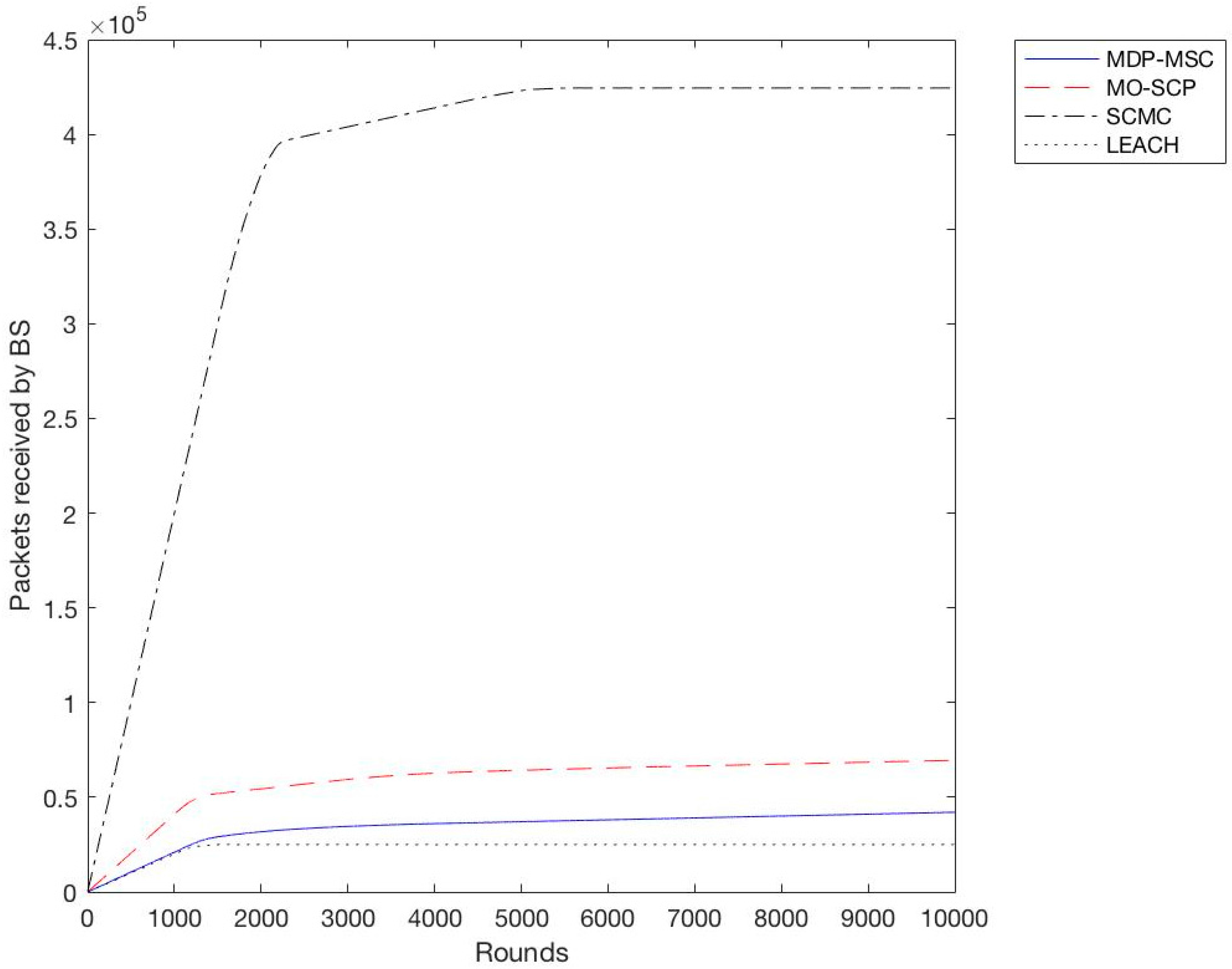
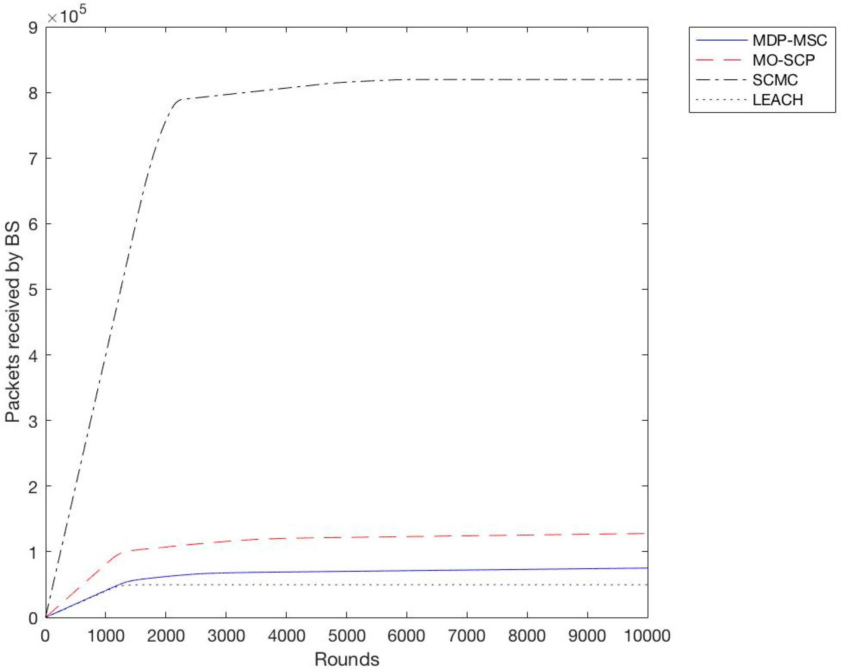
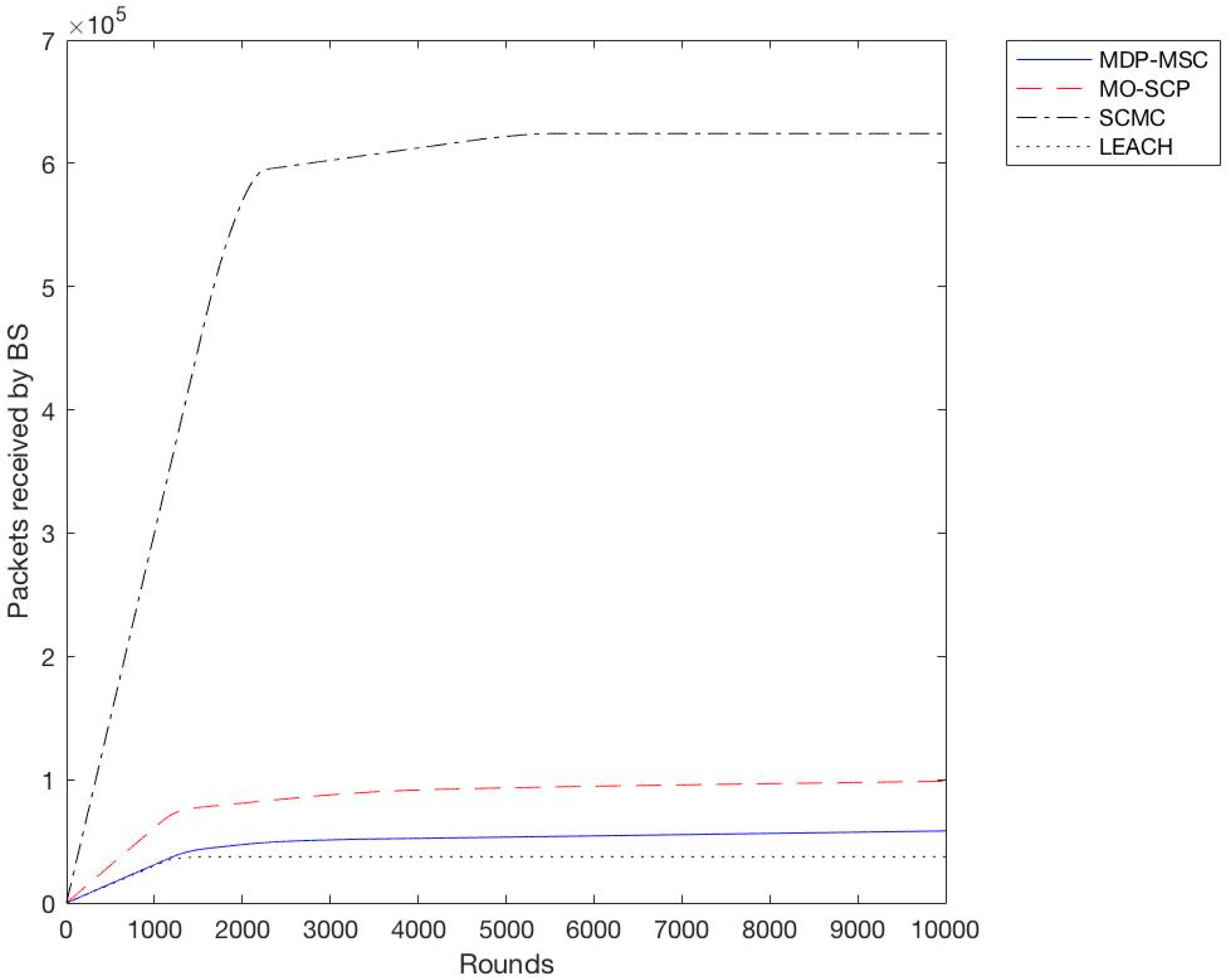
In the second experiment we calculated the throughput for all schemes with a different variation of sensor nodes from 100 to 400 with an increment of 100. We observe as shown in Figure 6, Figure 7, Figure 8 and Figure 9 that SCMC outperforms other algorithms in terms of a higher throughput and a larger number of packets received at the base station, which is understandable as SCMC has a longer lifetime and it uses an optimized routing path compared to other algorithms.

Figure 6. Throughput comparison of Set Cover Min-Cost max-flow (SCMC), Multi-Objective Set Cover Problem (MO-SCP), Minimum Distance Path-Maximum Set Cover (MDP-MSC), and Low-Energy Adaptive Clustering Hierarchy (LEACH) (Size = 100).

Figure 7. Throughput comparison of SCMC, MO-SCP, MDP-MSC and LEACH (Size = 200).

Figure 8. Throughput comparison of SCMC, MO-SCP, MDP-MSC and LEACH (Size = 300).

Figure 9. Throughput comparison of SCMC, MO-SCP, MDP-MSC and LEACH (Size = 400).

Based on the previous simulation results, we have shown that SCMC provides a higher throughput and a prolonged lifetime of the WSN compared to MO-SCP, MDP-MSC, and LEACH. This is due to the fact that SCMC uses a set cover approach to create clusters, and min-cost max-flow to route data between CHs and the base station. Although MDP-MSC also uses the concept of set covers to create clusters, it remains different from MO-SCP and SCMC in three ways. Firstly, it searches for k paths from the sink to all sensor nodes while MO-SCP and SCMC use a single path approach. Secondly, it calculates maximum disjoint set covers while MO-SCP and SCMC calculate a minimum set cover. Furthermore, MDP-MSC doesn’t consider the problem of extending the lifetime of WSNs as an optimization problem, while MO-SCP considers it as a multi-objective optimization problem, and SCMC as a single objective problem. In SCMC the energy consumption is well distributed among nodes and routing is done in an efficient way.

5. Conclusions

In this paper, we extensively studied the problem of minimizing the energy consumption and maximizing the lifetime of WSNs. For this purpose, an effective approach was presented using an optimization model. The proposed approach controls the energy depletion of sensor nodes and minimizes the routing path using the residual energy of the nodes. The corresponding optimization objective functions were solved using linear programing, and the simulation results showed that the proposed scheme (SCMC) outperforms MO-SCP, MDP-MSC, and LEACH in terms of WSN lifetime and throughput. As a future project, we intend to apply our approach to various base station scenarios. Additionally, the use of a multi-objective optimization model would be of great interest.