Cost-Aware IoT Extension of DISSECT-CF


Abstract
1. Introduction
2. Related Work
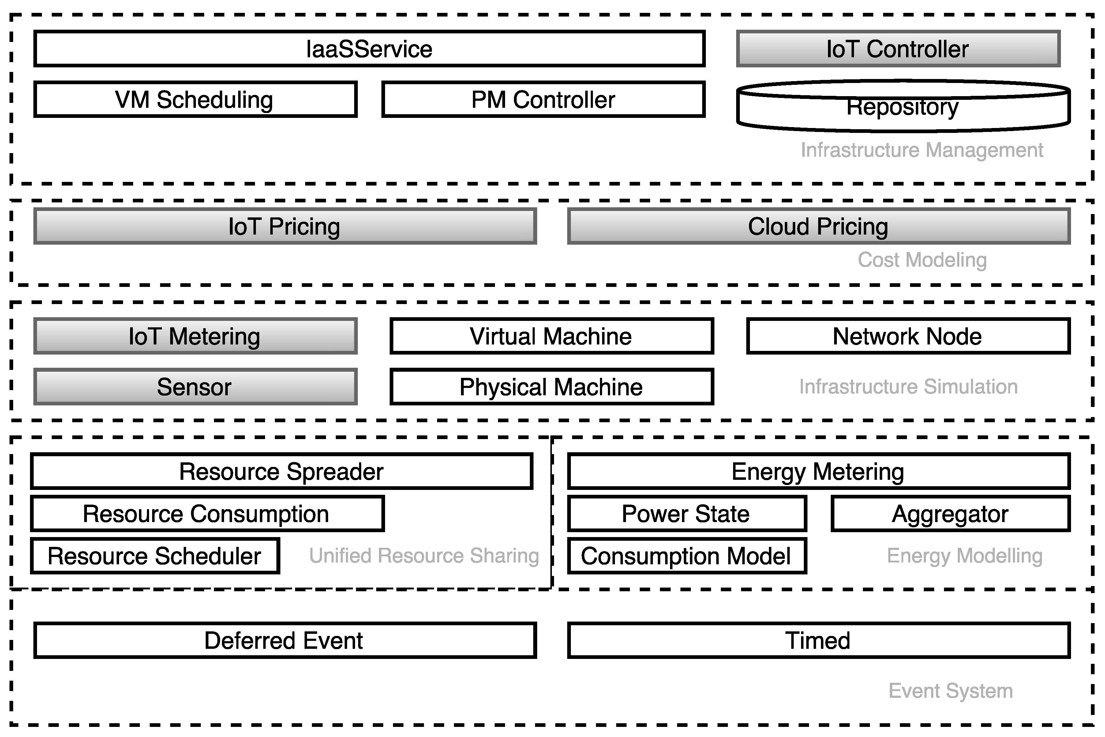
3. Cost Modeling in DISSECT-CF
3.1. IoT Pricing
3.1.1. Azure IoT Hub
3.1.2. IBM Bluemix
3.1.3. Amazon’s IoT platform
3.1.4. Oracle’s IoT Platform
3.2. Cloud Pricing
3.3. Configurable Cost Models
4. Implementation and Validation
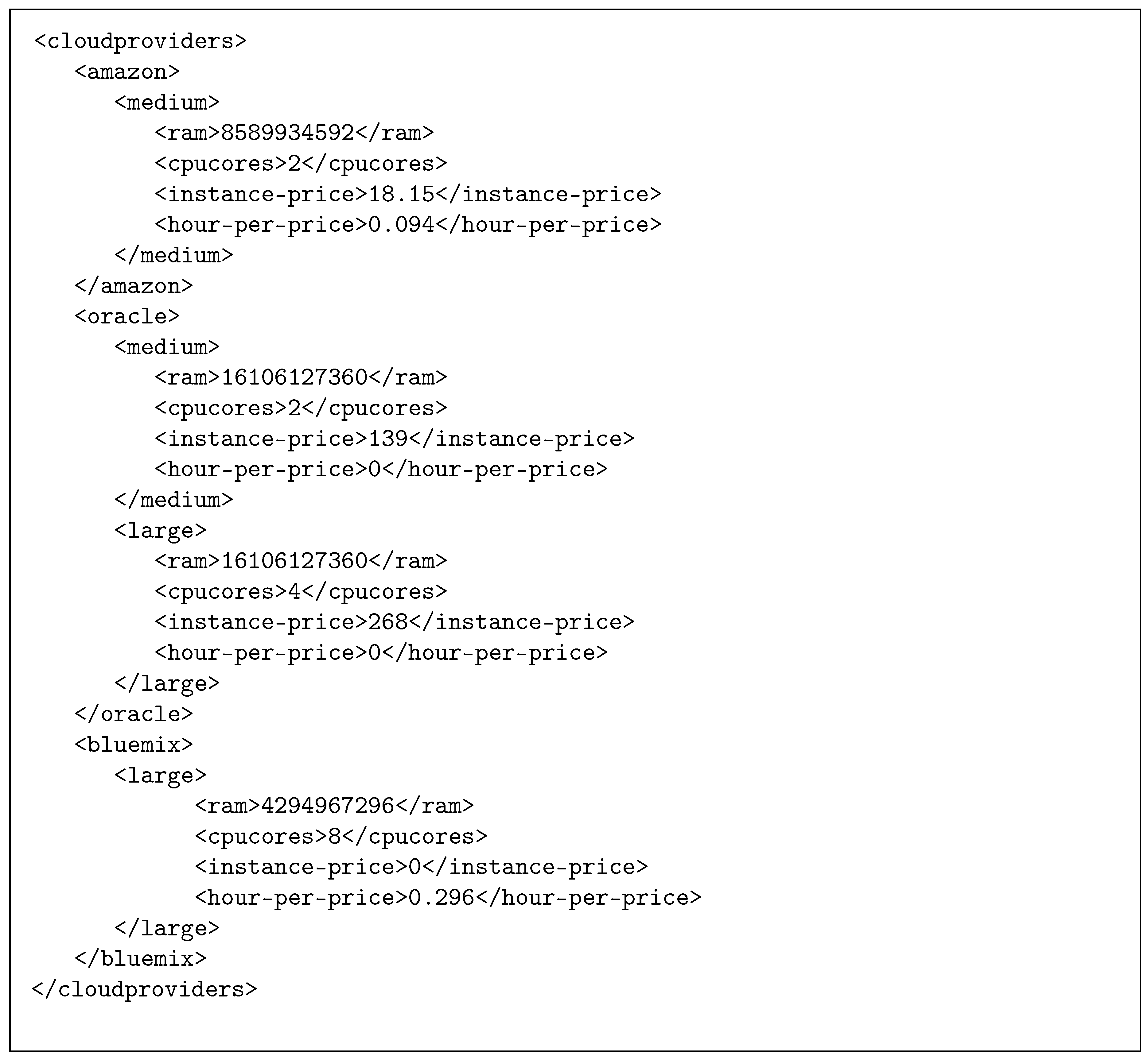
- Step 1: Set up the cloud using an XML. As we expect meteorological scenarios will often use private clouds, we used the model of a Hungarian private infrastructure (the LPDS (Laboratory of Parallel and Distributed Systems) Cloud of MTA SZTAKI (Institute for Computer Science and Control, Hungarian Academy of Sciences).
- Step 2: Set up the necessary amount of stations (using a scenario specific XML description) with the previously listed eight sensors per station.
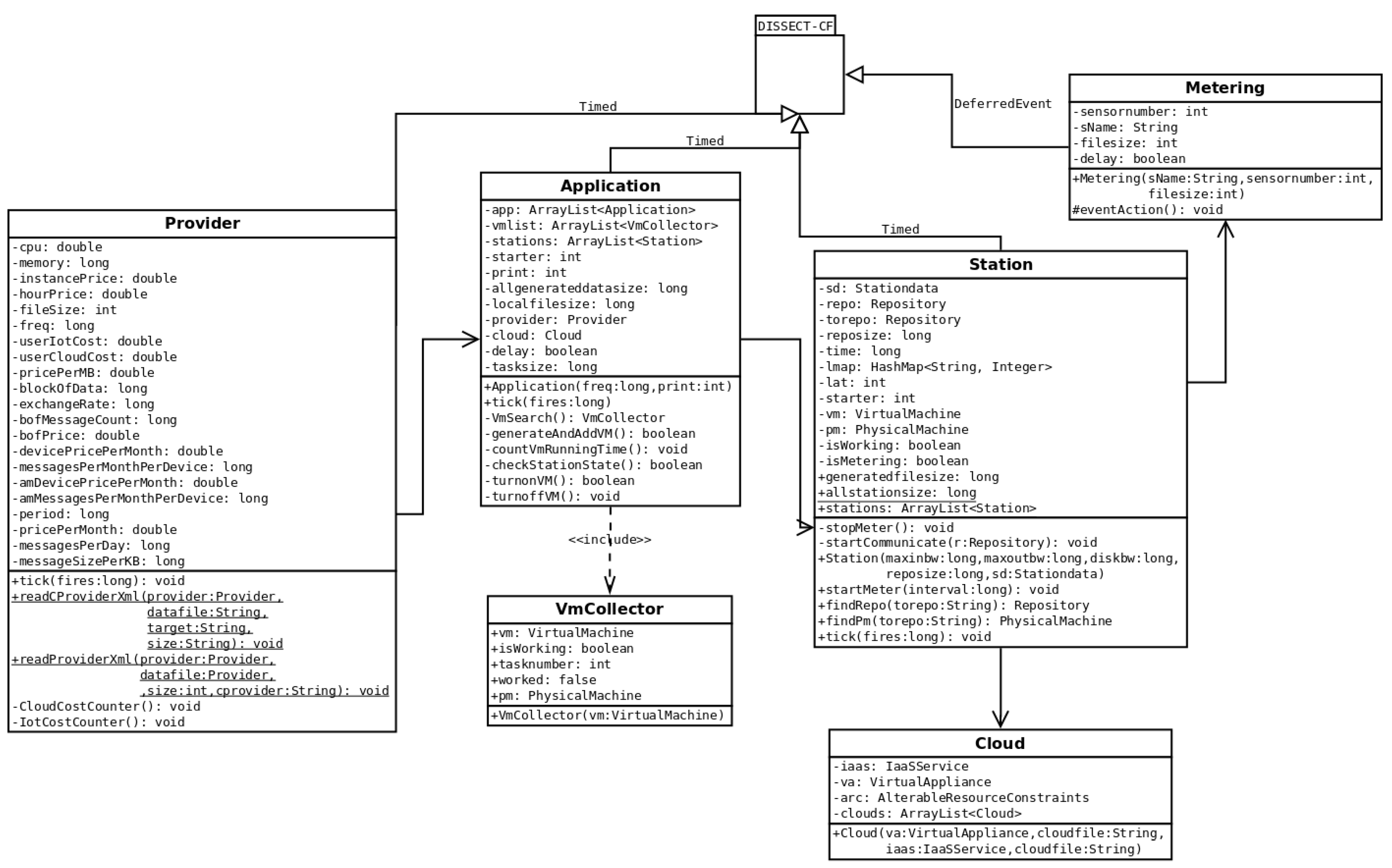
- Step 3: Load the VM parameters from XML files, which also describe the cloud and IoT costs. Start the Application to deploy an initial VM (generateAndAddVM()) for data processing and to start the metering process in all stations (startStation()).
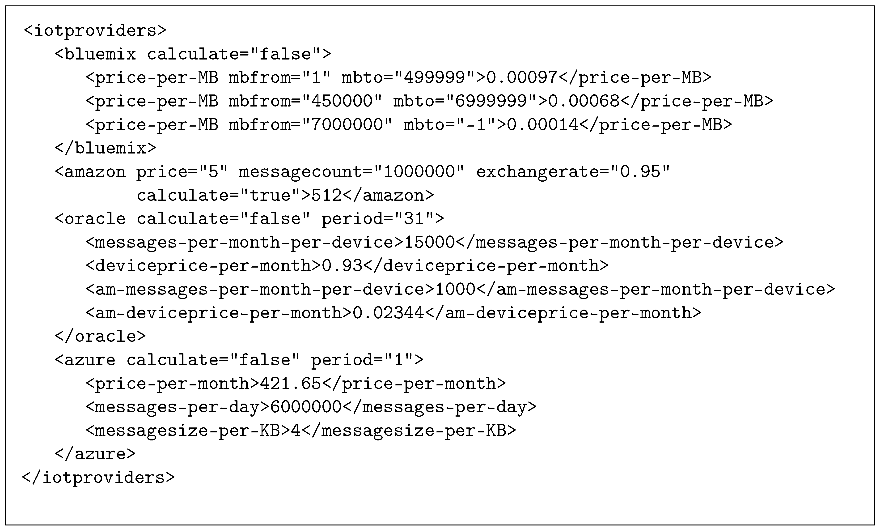
- Step 4: The stations then monitor (Metering()), save and send (startCommunicate()) sensor data (to the cloud storage) according to their XML definition. Parallel to this, CloudCostCounter() and IoTCostCounter() methods estimate the price of IoT and cloud operation, based on the generated data and processing of those data. The process of cost calculation depends on the chosen provider. If provider pricing is not time-dependent, like in case of Bluemix, we have to pay only after data traffic, then this loop is executed only once, at the end of the simulation. Otherwise, if the provider cost is time-dependent, the time interval for the measurements is given in the period attribute, as shown in Figure 2. This interval represents the frequency value to be used by the extended provider class, and the corresponding cost counter methods are executed in all cycles.
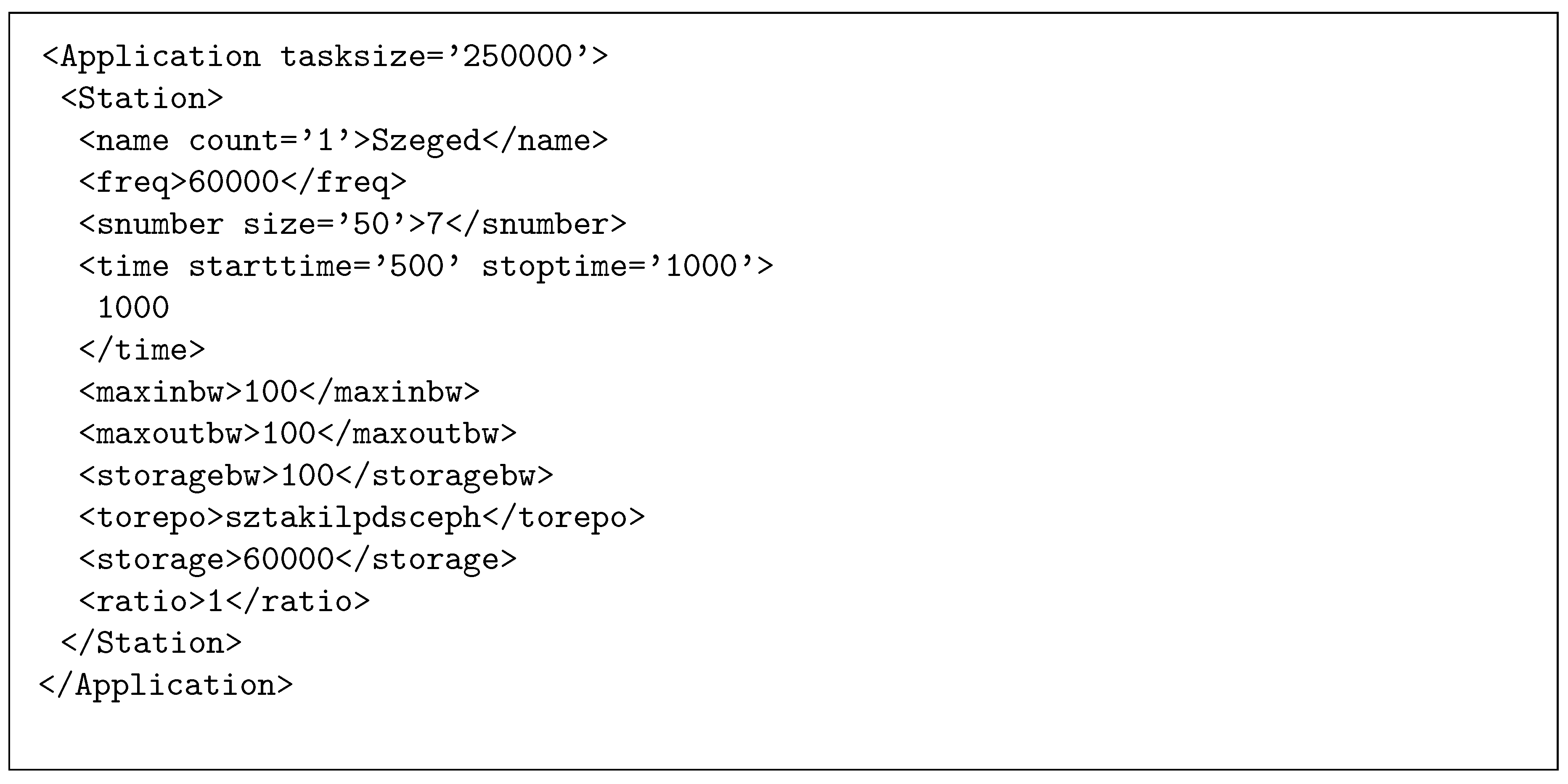
- Step 5: A daemon service checks regularly if the cloud repository received a scenario specific amount of data (see the tasksize attribute in Figure 5). If so, then the Application generates the ingest compute tasks, which will finish processing within a predefined amount of time.
- Step 6: Next, for each generated task, a free VM is searched (by VmSearch()). If a VM is found, the task and the relevant data is sent to it for processing.
- Step 7: In case there are no free VMs found, the daemon initiates a new VM deployment and holds back the not yet mapped tasks.
- Step 8: If at the end of the task assignment phase, there are still free VMs, they are all decommissioned (by turnoffVM()), except those that are held back for the next rounds (this amount can be configured and even completely turned off at will).
- Step 9: Finally, the Application returns to Step 5.
Evaluation with Five Scenarios
5. Conclusions
Supplementary Materials
Acknowledgments
Author Contributions
Conflicts of Interest
References
- Sotiriadis, S.; Bessis, N.; Asimakopoulou, E.; Mustafee, N. Towards simulating the Internet of Things. In Proceedings of the IEEE 28th International Conference on Advanced Information Networking and Applications Workshops (WAINA), Cracow, Poland, 16–18 May 2014; pp. 444–448. [Google Scholar]
- Han, S.N.; Lee, G.M.; Crespi, N.; Heo, K.; Van Luong, N.; Brut, M.; Gatellier, P. DPWSim: A simulation toolkit for IoT applications using devices profile for web services. In Proceedings of the IEEE World Forum on IoT (WF-IoT), Seoul, Korea, 6–8 March 2014; pp. 544–547. [Google Scholar]
- Zeng, X.; Garg, S.K.; Strazdins, P.; Jayaraman, P.P.; Georgakopoulos, D.; Ranjan, R. IOTSim: A simulator for analysing IoT applications. J. Syst. Archit. 2016, 72, 93–107. [Google Scholar] [CrossRef]
- Kecskemeti, G. DISSECT-CF: A simulator to foster energy-aware scheduling in infrastructure clouds. Simul. Model. Pract. Theory 2015, 58P2, 188–218. [Google Scholar] [CrossRef]
- Kecskemeti, G.; Nemeth, Z. Foundations for Simulating IoT Control Mechanisms with a Chemical Analogy. In Internet of Things, Proceeding of the IoT 360° 2015, Rome, Italy, 27–29 October 2015. Revised Selected Papers, Part I; Mandler, B., Marquez-Barja, J., Eds.; Springer International Publishing: New York, NY, USA, 2016; Volume 169, pp. 367–376. [Google Scholar]
- Idokep.hu Website. Available online: http://idokep.hu (accessed on 13 August 2017).
- Sotiriadis, S.; Bessis, N.; Antonopoulos, N.; Anjum, A. SimIC: Designing a new Inter-Cloud Simulation platform for integrating large-scale resource management. In Proceedings of the IEEE 27th International Conference on Advanced Information Networking and Applications (AINA), Barcelona, Spain, 25–28 March 2013; pp. 90–97. [Google Scholar]
- Moschakis, I.A.; Karatza, H.D. Towards scheduling for Internet-of-Things applications on clouds: A simulated annealing approach. Concurr. Comput. 2015, 27, 1886–1899. [Google Scholar] [CrossRef]
- Silva, I.; Leandro, R.; Macedo, D.; Guedes, L.A. A dependability evaluation tool for the Internet of Things. Comput. Electr. Eng. 2013, 39, 2005–2018. [Google Scholar] [CrossRef]
- Khan, A.M.; Navarro, L.; Sharifi, L.; Veiga, L. Clouds of small things: Provisioning infrastructure-as-a-service from within community networks. In Proceedings of the IEEE 9th International Conference on Wireless and Mobile Computing, Networking and Communications (WiMob), Lyon, France, 7–9 October 2013; pp. 16–21. [Google Scholar]
- Calheiros, R.N.; Ranjan, R.; Beloglazov, A.; De Rose, C.A.; Buyya, R. CloudSim: A toolkit for modeling and simulation of cloud computing environments and evaluation of resource provisioning algorithms. Software 2011, 41, 23–50. [Google Scholar] [CrossRef]
- Botta, A.; De Donato, W.; Persico, V.; Pescapé, A. On the integration of cloud computing and internet of things. In Proceedings of the IEEE International Conference on Future Internet of Things and Cloud, Barcelona, Spain, 27–29 August 2014; pp. 23–30. [Google Scholar]
- Nastic, S.; Sehic, S.; Le, D.H.; Truong, H.L.; Dustdar, S. Provisioning software-defined iot cloud systems. In Proceedings of the IEEE International Conference on Future Internet of Things and Cloud, Barcelona, Spain, 27–29 August 2014; pp. 288–295. [Google Scholar]
- Giacobbe, M.; Puliafito, A.; Pietro, R.D.; Scarpa, M. A Context-Aware Strategy to Properly Use IoT-Cloud Services. In Proceedings of the 2017 IEEE International Conference on Smart Computing (SMARTCOMP), Hong Kong, China, 29–31 May 2017; pp. 1–6. Available online: http://dx.doi.org/10.1109/SMARTCOMP.2017.7946976 (accessed on 1 July 2017).
- DISSECT-CF Website. Available online: https://github.com/kecskemeti/dissect-cf (accessed on 13 August 2017).
- MS Azure IoT Hub Website. Available online: https://azure.microsoft.com/en-us/services/iot-hub (accessed on 13 August 2017).
- IBM Bluemix Website. Available online: https://www.ibm.com/cloud-computing/bluemix/internet-of-things (accessed on 13 August 2017).
- Amazon AWS IoT Website. Available online: https://aws.amazon.com/iot/pricing (accessed on 13 August 2017).
- Oracle IoT Platform Website. Available online: https://cloud.oracle.com/en_US/opc/iot/pricing (accessed on 13 August 2017).
- MS Azure Price Calculator. Available online: https://azure.microsoft.com/en-gb/pricing/calculator/ (accessed on 13 August 2017).
- IBM Bluemix Pricing Sheet. Available online: https://www.ibm.com/cloud-computing/bluemix (accessed on 13 August 2017).
- Amazon Pricing Website. Available online: https://aws.amazon.com/ec2/pricing/on-demand/ (accessed on 13 August 2017).
- Oracle Pricing Website. Available online: https://cloud.oracle.com/en_US/opc/compute/compute/pricing (accessed on 13 August 2017).
- Orcale Metered Services Pricing Calculator. Available online: https://shop.oracle.com/cloudstore/index.html?product=compute (accessed on 13 August 2017).
- Murdoch University Weather Station Website. Available online: http://wwwmet.murdoch.edu.au/downloads (accessed on 13 August 2017).
- DISSECT-CF Extension Scenarios. Available online: https://github.com/andrasmarkus/dissect-cf/tree/andrasmarkus-patch-1/experiments (accessed on 13 August 2017).
- Markus, A.; Kecskemeti, G.; Kertesz, A. Flexible Representation of IoT Sensors for Cloud Simulators. In Proceedings of the 25th Euromicro International Conference on Parallel, Distributed and Network-based Processing (PDP), St. Petersburg, Russia, 6–8 March 2017; pp. 199–203. [Google Scholar]


| Amount of Data (Byte) | Number of VMs | Number of Tasks | Produced Data (GB) |
|---|---|---|---|
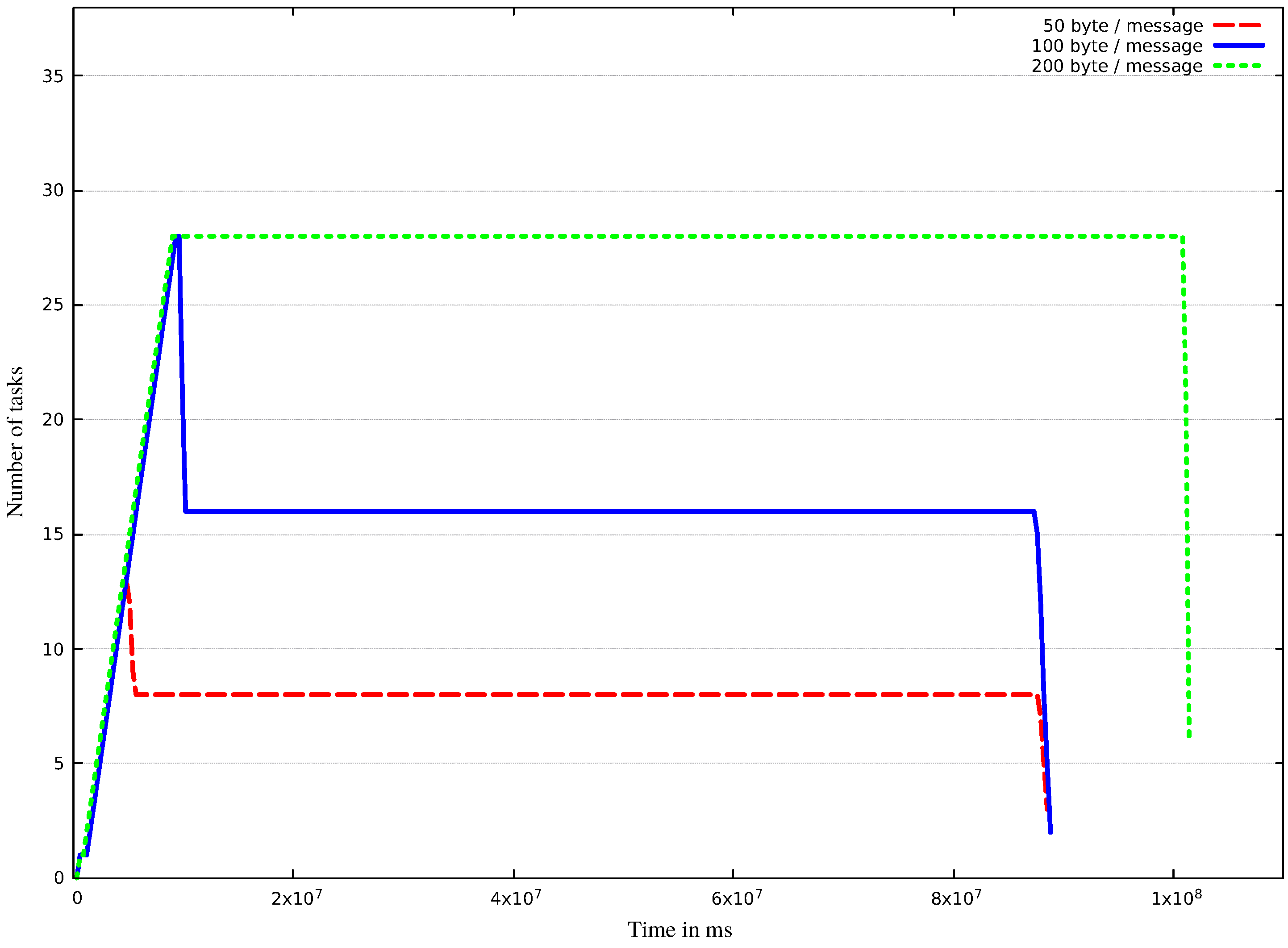
| 50 | 12 | 1153 | 0.261 |
| 100 | 27 | 2299 | 0.522 |
| 200 | 28 | 4486 | 1.044 |
| Station Type | Number of VMs | Number of Tasks | Produced Data (GB) |
|---|---|---|---|
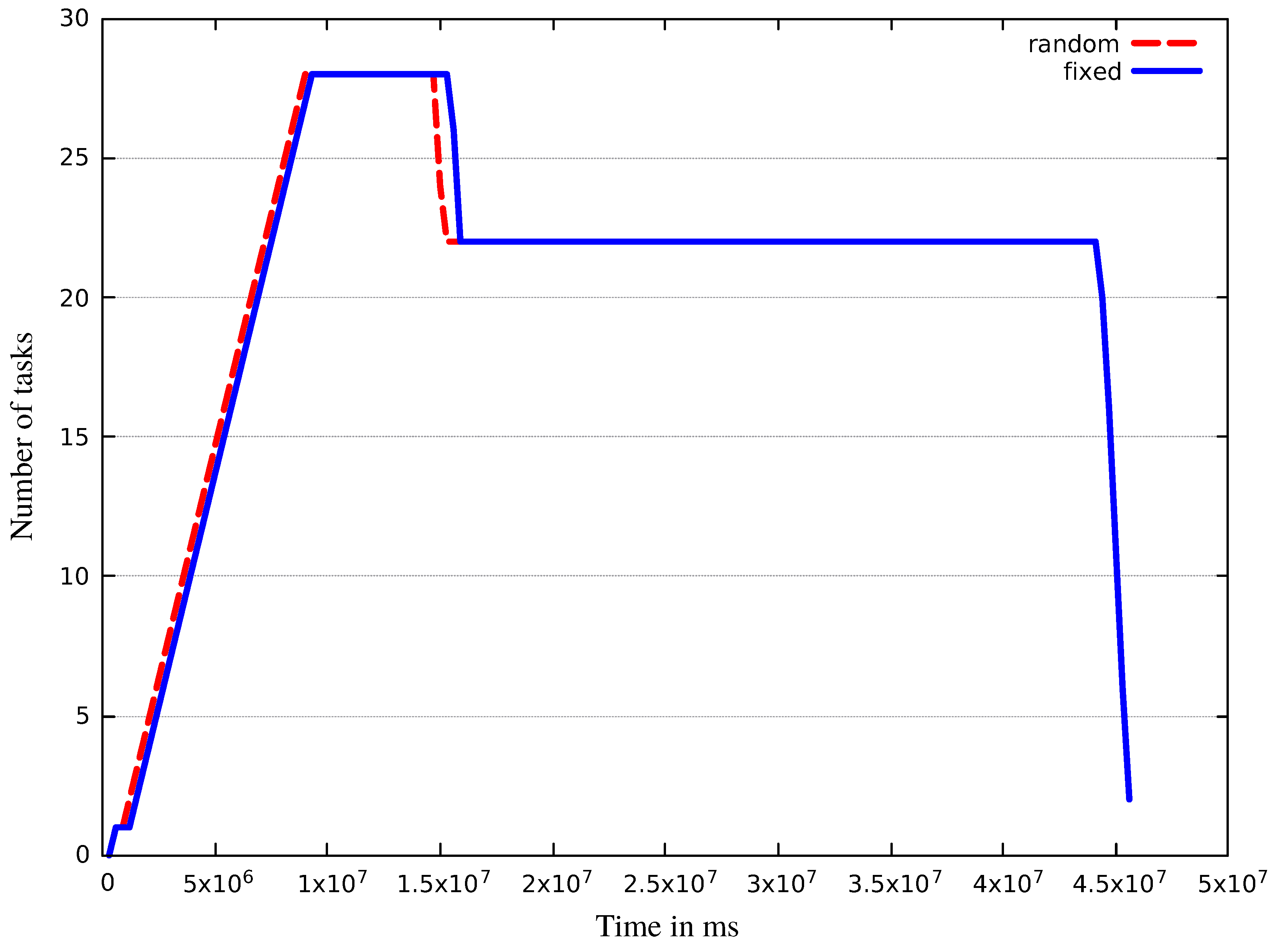
| fixed | 28 | 1555 | 0.348 |
| random | 28 | 1561 | 0.352 |
| VM Category | Small | |||||||
|---|---|---|---|---|---|---|---|---|
| Interval | 1 min | 5 min | ||||||
| Azure cloud cost | 20.039 | 4.200 | ||||||
| IoT provider | Bluemix | Amazon | Oracle | Azure | Bluemix | Amazon | Oracle | Azure |
| IoT side cost | 0.31948 | 32.80 | 4464.00 | 4215.5 | 0.06371 | 6.5436 | 4464.00 | 4215.5 |
| Sum | 20.35848 | 52.839 | 4484.039 | 4235.539 | 4.26371 | 10.7436 | 4468.2 | 4219.7 |
| VM Category | Medium | |||||||
|---|---|---|---|---|---|---|---|---|
| Interval | 1 min | 5 min | ||||||
| Azure cloud cost | 32.538 | 5.45 | ||||||
| IoT provider | Bluemix | Amazon | Oracle | Azure | Bluemix | Amazon | Oracle | Azure |
| IoT side cost | 0.31948 | 32.80 | 4464.00 | 4215.5 | 0.06371 | 6.5436 | 4464.00 | 4215.5 |
| Sum | 32.85748 | 65.338 | 4496.538 | 4248.038 | 5.51371 | 11.9936 | 4469.45 | 4220.95 |
| VM Category | Large | |||||||
|---|---|---|---|---|---|---|---|---|
| Interval | 1 min | 5 min | ||||||
| Azure cloud cost | 62.667 | 7.128 | ||||||
| IoT provider | Bluemix | Amazon | Oracle | Azure | Bluemix | Amazon | Oracle | Azure |
| IoT side cost | 0.31948 | 32.80 | 4464.00 | 4215.5 | 0.06371 | 6.5436 | 4464.00 | 4215.5 |
| Sum | 62.98648 | 95.467 | 4526.667 | 4278.167 | 7.19171 | 13.6716 | 4471.128 | 4222.628 |
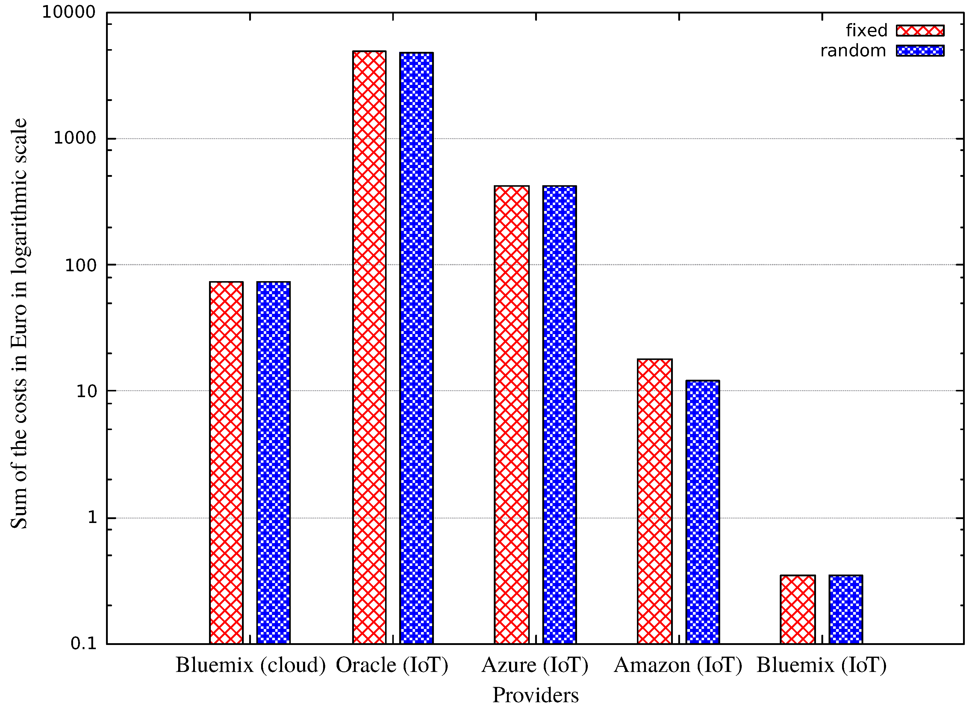
| IoT Provider | Bluemix | Amazon | Oracle | Azure | ||||
|---|---|---|---|---|---|---|---|---|
| IoT side cost | 0.18 | 18.92 | 14136.00 | 421.65 | ||||
| VM function | ON | OFF | ON | OFF | ON | OFF | ON | OFF |
| Bluemix cloud cost | 51.80 | 89.39 | 51.80 | 89.39 | 51.80 | 89.39 | 51.80 | 89.39 |
| Sum | 51.98 | 89.58 | 70.72 | 108.31 | 14187.80 | 14225.39 | 473.45 | 511.04 |
© 2017 by the authors. Licensee MDPI, Basel, Switzerland. This article is an open access article distributed under the terms and conditions of the Creative Commons Attribution (CC BY) license (http://creativecommons.org/licenses/by/4.0/).
Share and Cite
Markus, A.; Kertesz, A.; Kecskemeti, G. Cost-Aware IoT Extension of DISSECT-CF. Future Internet 2017, 9, 47. https://doi.org/10.3390/fi9030047
Markus A, Kertesz A, Kecskemeti G. Cost-Aware IoT Extension of DISSECT-CF. Future Internet. 2017; 9(3):47. https://doi.org/10.3390/fi9030047
Chicago/Turabian StyleMarkus, Andras, Attila Kertesz, and Gabor Kecskemeti. 2017. "Cost-Aware IoT Extension of DISSECT-CF" Future Internet 9, no. 3: 47. https://doi.org/10.3390/fi9030047
APA StyleMarkus, A., Kertesz, A., & Kecskemeti, G. (2017). Cost-Aware IoT Extension of DISSECT-CF. Future Internet, 9(3), 47. https://doi.org/10.3390/fi9030047