A Novel DOA Estimation Algorithm Using Array Rotation Technique

Abstract

The performance of traditional direction of arrival (DOA) estimation algorithm based on uniform circular array (UCA) is constrained by the array aperture. Furthermore, the array requires more antenna elements than targets, which will increase the size and weight of the device and cause higher energy loss. In order to solve these issues, a novel low energy algorithm utilizing array base-line rotation for multiple targets estimation is proposed. By rotating two elements and setting a fixed time delay, even the number of elements is selected to form a virtual UCA. Then, the received data of signals will be sampled at multiple positions, which improves the array elements utilization greatly. 2D-DOA estimation of the rotation array is accomplished via multiple signal classification (MUSIC) algorithms. Finally, the Cramer-Rao bound (CRB) is derived and simulation results verified the effectiveness of the proposed algorithm with high resolution and estimation accuracy performance. Besides, because of the significant reduction of array elements number, the array antennas system is much simpler and less complex than traditional array.

2. The MUSIC Algorithm of 2-D UCA

Consider a UCA with M elements impinged by D narrowband signals s_i(t), i = 1, 2, …, D (D < M), where t is the time variable, as shown in Figure 1. The D sources are assumed to be from far-field with azimuth θ_i and elevation φ_i, i = 1, 2, …, D. Assume the radius of UCA is r and the noise is additive white Gaussian noise (AWGN).

Figure 1. Uniform circular array diagram.

Consider the reference point is 0, the ideal steering matrix can be obtained from the array geometry as

A(θ,φ) = [a(θ₁,φ₁), a(θ₂,φ₂), ⋯, a(θ_D,φ_D)]

(1)

a(θ_i,φ_i) = [a₁(θ_i,φ_i),a₂(θ_i,φ_i), ⋯, a_M (θ_i,φ_i)]^T

(2)

a_k (θ_i,φ_ki) = exp(− jωτ_i) = exp(− j dr cos (2π(k − 1)/ M − θ_i) cos φ_i)

(3)

where k = 1, 2, …, M; i = 1, 2, …, D; λ is wavelength; d = 2π/λ. The array output of the kth element at time t can be written as

(4)

Equation (4) can be written in matrix form as

X(t)=AS(t)+N(t)

(5)

where X(t) is M × 1 array output vector; A is M × D array steering matrix; S(t) is D × 1 signal vector; N(t) is M × 1 noise vector. X(t), S(t) and N(t) are abbreviated as X, S and N, respectively, and the array covariance matrix of X can be written as

R = E[XX^H]=APA^H+σ²I

(6)

where P = E[SS^H] = diag[P₁, P₂, …, P_i, …, P_D]; P_i is the power of the ith signal; σ² is noise power; I is M × 1 identity matrix. E[•] and [•]^H denote the statistical expectation and the Hermitian transpose, respectively. In real systems, the covariance matrix R can be estimated from a finite set of sample snapshots as

(7)

where L is the total number of snapshots. Then the eigendecomposition of can be written as

(8)

where ∑ = diag{λ₁ ≥ λ₂, ⋯, λ_M}; λ_i and v_i are the eigenvalue and corresponding eigenvector of , respectively. In ideal conditions, λ₁ ≥ λ₂ ⋯ ≥ λ_D ≥ λ_{D +1} = ⋯ = λ_M = σ². Assume that the number of incident signals D is known, can be described as

(9)

where U_S = [v₁, v₂, ⋯, v_D] and U_N = [v_D+1, v_D+2, ⋯, v_M] are the signal subspace and noise subspace, respectively; ∑_S = diag{λ_1, ⋯, λ_D} and ∑_N = diag{λ_D+1, ⋯, λ_M} are diagonal matrices related to the signal and noise power, respectively. Because the D-incident sources spanning the signal space are orthogonal to the noise space, so the MUSIC algorithm can estimate the DOA as

(10)

where P_MUSIC (θ,φ) is expected to show a large positive value if (θ,φ) is a true DOA, because a^H (θ,φ) v_i = 0, i = D +1, ⋯, M. Here, the signal is processed before the data is demodulated, where the carrier phase information is maintained through the sampling.

3. The Proposed Algorithm

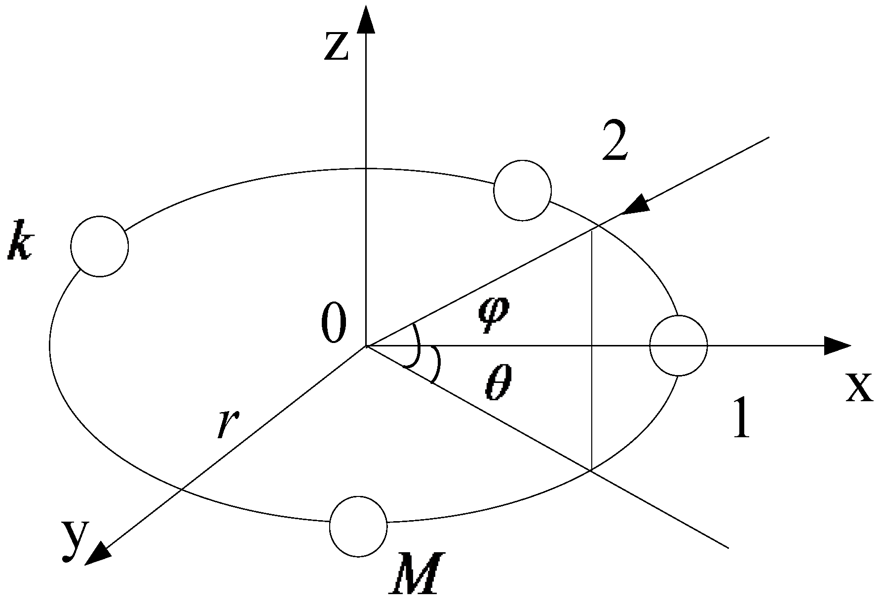
3.1. The Rotation Array Structure of Proposed Algorithm

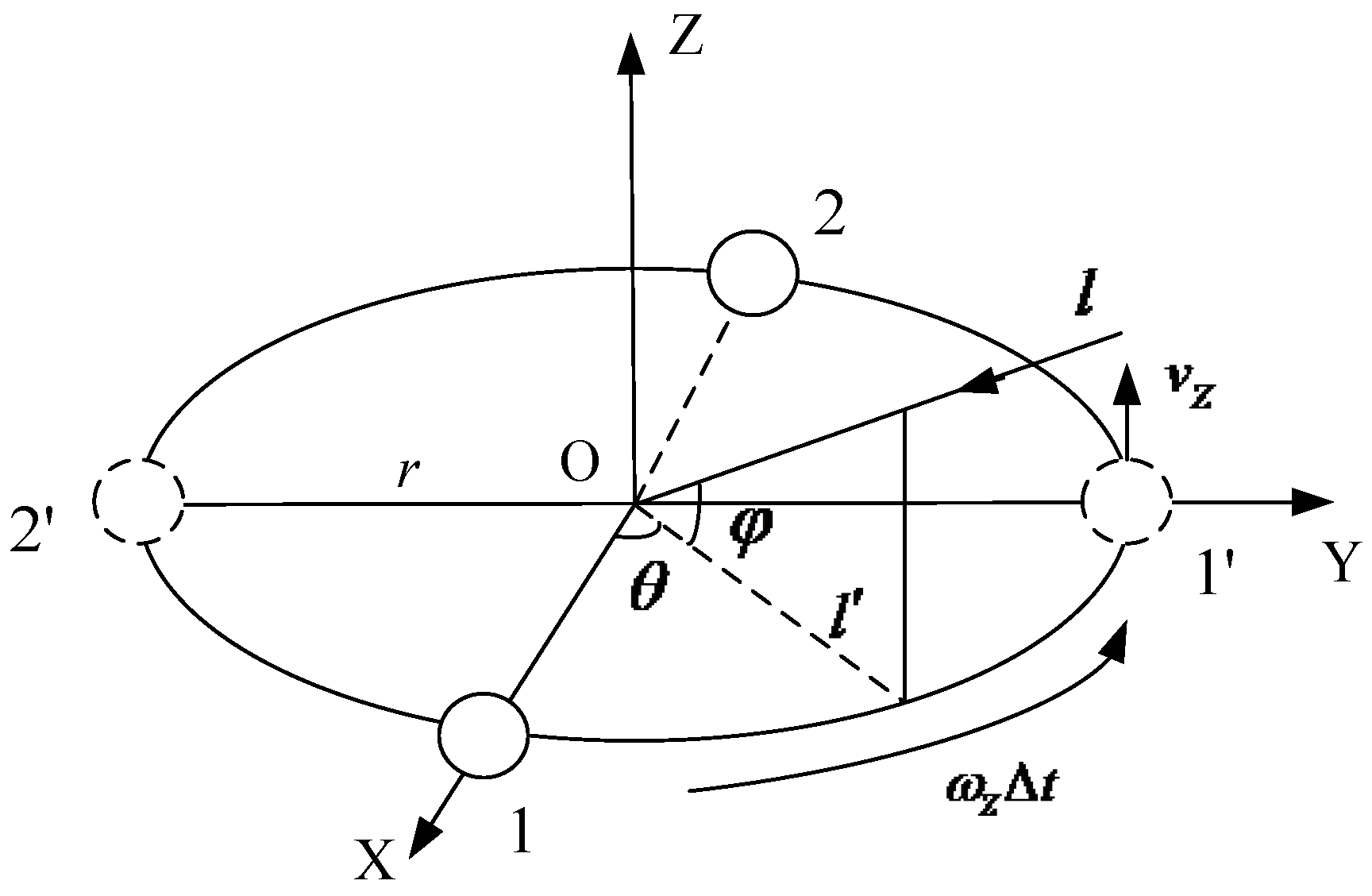
As shown in Figure 2, D narrowband far-field sources are observed by a rotation array with two antenna elements, “1” and “2”. Assume the baseline 1–2 is rotating around Z-axis in XOY plane at a constant velocity by anticlockwise direction. The rotate velocity is v_Z, v_Z = ω_Zr = 2πƒ_zr, where ω_Z is rotational angular frequency; ƒ_z is rotation frequency. The rotation period is T. After time Δt (Δt < T), the elements 1 and 2 are rotating to the position 1ʹ and 2ʹ, respectively. Assume the array radius is r; l is the incident signal direction; lʹ is the projection of l onto the XOY plane; θ and φ are azimuth and elevation, respectively.

Figure 2. Rotation array structure diagram.

In order to derive the proposed algorithm, some assumptions are clarified at first,

(1)

While the baseline 1–2 is rotating, the baseline is certainly vertical to Z-axis with absolute uniform velocity;

(2)

Select 2M elements at uniformly-time interval to make them form the virtual UCA within T/2 period;

(3)

The signals remain static during the measurement time.

At time t_m, the elements 1 and 2 start to sample the received signal data, so t_m can be expressed as

t_m = t₁ + (m − 1)∆τ

(11)

where t₁ = 0, m = 1,2, ⋯,M ; ∆τ is the time delay which is needed for selecting two neighboring elements, 0 < ∆τ < T / 2. As we know, the wave path difference between the reference point O and the mth element for the ith signal is τ_mi. In the rotation array model, the element m is obtained by rotating element 1 through time (m − 1)∆τ, so the total wave path difference τ_1m is

τ_1m = τ_mi + (m−1) _∆τ

(12)

(12)

Then Equation (4) is modified as

(13)

Assuming the signal sources remain static, the element rotation will cause the Doppler frequency shift. As shown in Figure 2, v is denoted as the velocity component of v_z in the source incident direction Ɩʹ, we obtain

v = v_z sin(θ − ω_zt) cos φ

(14)

According to the Doppler frequency formula ƒ_d = v•ƒ /c, ƒ_d can be written as

ƒ_d = v_z sin(θ − ω_zt) cos φ •ƒ /c
= 2πƒ_zr sin(θ − ω_zt) cos φ •ƒ / c

(15)

where ƒ is signal frequency. Therefore, in (13), ω should be modified as

ω = 2π(ƒ + ƒ_d)

(16)

Let ϕ_tm = exp(− j ω(m − 1)∆τ), the vector received by element 1 within T/2 period can be expressed by

(17)

where ϕ_tm is the phase difference of element 1 at time t_m relative to the initial position. Equation (17) can be further simplified as

(18)

where X₁ = [x₁₁, x₁₂, ⋯, x_1M]^T is M × 1 array output matrix; N₁ = [n₁(t₁), n₁(t₂), ⋯, n₁(t_M)]^T is M × 1 noise matrix. The steering matrix A₁ can be written as

A₁ = [a₁(θ₁, φ₁), a₁(θ₂, φ₂), ⋯, a₁(θ_D, φ_D)]

(19)

a₁(θ_j, φ_j) = [a₁₁(θ₁, φ₁), a₁₂(θ₂, φ₂), ⋯, a_1M (θ_D, φ_D)]^T

(20)

where a_1m(θ_i,φ_i) = exp(− j ωτ_mi); ; m = 1,2⋯, M; i = 1,2, ⋯, D.

Denote Φ₁ = diag[ϕ_t1,ϕ_t2, ⋯, ϕ_tM], (17) can be expressed by

X₁ = Φ₁A₁S + N₁

(21)

In the same way, the vector received by element 2 within T/2 period is

(22)

Similarly, denoting Φ₂ = diag[ϕ_t1, ϕ_t2, ⋯, ϕ_tM]; ϕ_tm is the phase difference of element 2 at time t_m relative to the initial position; therefore, the array output matrix of element 2 within T/2 is modeled as

X₂ = Φ₂A₂S + N₂

(23)

When the array elements are rotating more than T/2 period, we can select 2M elements to construct a virtual UCA. Then, integrate X₁ with X₂, X can be represented by X₁ and X₂

(24)

where .

Using Equations (7), (9) and (10), MUSIC spectrum function will be obtained.

Seen from the analysis above, the key advantages of the proposed method is, by sampling the received signal date at a uniform time interval while the array antennas are rotating, more than two antenna elements can be obtained and it can estimate more than two DOAs. Besides, because the number of antennas is much smaller, the array system is greatly simplified than the traditional array and it will become much easier to calibrate with channel phase errors in practice.

3.2. How to Choose Array Rotation Velocity

Consider the rotation frequency is ƒ_z, and ƒ_z = 1/T, ƒ_s is the sampling frequency of the receiver. Select 2M antenna elements within T/2 period while array rotating. Because the characteristics of element 1 are the same as element 2, we only need to analyze element 1 in this subsection. As we know, the received signal data is sampled while the array is rotating, which will cause a tiny phase difference between every two sampled data. In order to ensure the stability of sampled data, ∆τ should satisfy the following equation

(25)

where ∆τ is much greater than the sampling time interval. We have

(26)

Assume the snapshots is L, then

(27)

(28)

As a result, if (28) is satisfied, the stability of the algorithm could be ensured. Consider the sampling frequency of a receiver is 50 MHz, the elements number is 8, the snapshots number L is 100, according to (28), we can get ƒ_z ≪ 31 250 Hz. If the antenna rotation frequency is much smaller than 31,250 Hz, the stability of the sampled data will be guaranteed.

4. The Cramer-Rao Bound

Cramer-Rao bound (CRB) gives a lower bound of unbiased parameter estimation. In this section, some assumptions are considered to hold throughout this section first: (1) The number of selected array elements should be greater than that of signals (M > D); (2) The noise {n(t)} is Gaussian distributed and E{n(t)n^H(t)} = σ²I, E{n(t)n^T(t)} = 0; (3) The signal covariance matrix R_S = E{SS^H} is positive definite. Furthermore, the signals and noise are uncorrelated for all time. Under these conditions, we derive the Cramer-Rao bound (CRB) formula for the algorithm proposed in this paper. The derivation process approximates the method proposed in [24].

Define u is the angle parameters vector contained in the signal covariance matrix R_S,

u = [θ^T,φ^T]^T

(29)

where θ = [θ₁, ⋯, θ_D]^T, φ = [φ₁, ⋯, φ_D]^T. The CRB of the angle parameters is defined as

var(u) ≥ CRB

(30)

var(u) = E[(û - u)(û - u)^T]

(31)

CRB = F^-1

(32)

The 2D × 2D Fisher information matrix (FIM) for the parameter u is given by

(33)

where F_θθ is the block matrix of azimuth estimator and F_φφ is the block matrix of elevation estimator. The m, n elements of F is represented as

(34)

where trace[●] is the trace of matrix[●]. L is the snapshot. Define

G = [G_θ,G_φ]

(35)

(36)

(37)

Then the matrix F_θθ, F_φφ, F_φθ, F_θφ, is represented as

(38)

(39)

(40)

(41)

where ʘ denotes the Hadamard product.

5. Simulation Examples

This section demonstrates the performance of the proposed method via numerical simulation. In all simulation examples, we use the rotation array structure shown in Figure 2. The radius r is 0.124 m, the rotation frequency ƒ_z is 15 Hz, and the noise background is AWGN. Select M = 8 and M = 10 elements for forming the UCA to estimate DOAs. To verify the performance of the R-MUSIC algorithm, some comparison simulations of MUSIC algorithm with five elements UCA and eight elements UCA are carried as well.

5.1. Resolution Performance Simulation

In this part, the resolution is defined as

(42)

where θ_m = (θ₁ + θ₂)/ 2. When the right-hand side of (30) is smaller than the left-hand side, the two angles can be distinguished; while the right-hand sides of (30) is great than the left-hand sides, then the two angles cannot be distinguished. Furthermore, the successful resolution probability is defined as the ratio of successful test numbers to the total test numbers.

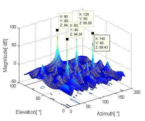
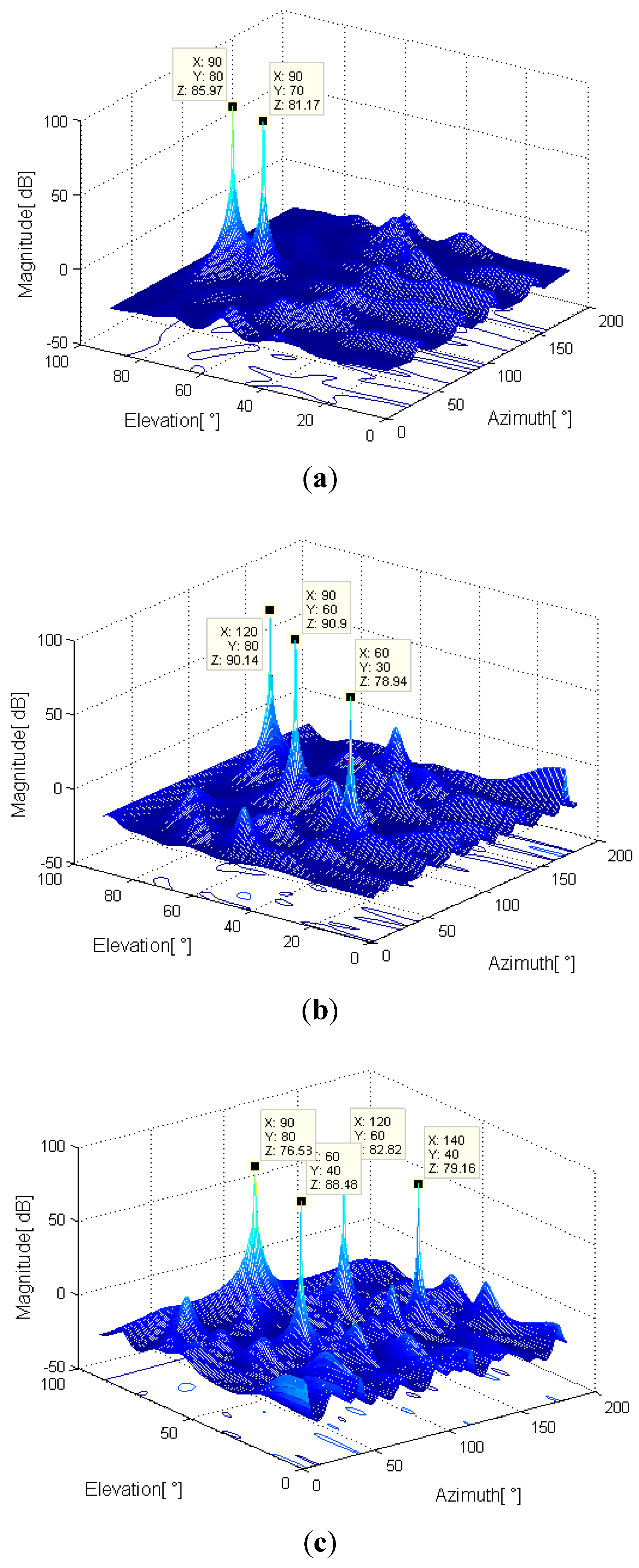
5.1.1. The Spatial Spectrum of the R-MUSIC Algorithm

In order to verify the effectiveness of the proposed method, some spatial spectrum figures are shown in this section. Assume there are several incoherent signals impinging on the array, the signal frequencies are 6 GHz, SNR (signal to noise ratio) is 20 dB and the snapshots are 100. Figure 3 shows the spatial spectrum of two, three, and four incident signals, respectively. It can be seen that the proposed method has better resolution and estimation accuracy performance. In addition, it can estimate more than two sources successfully.

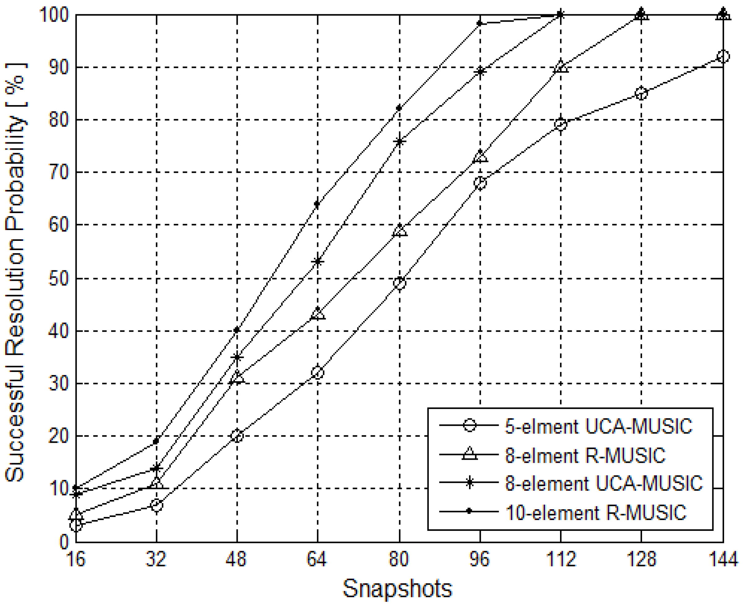
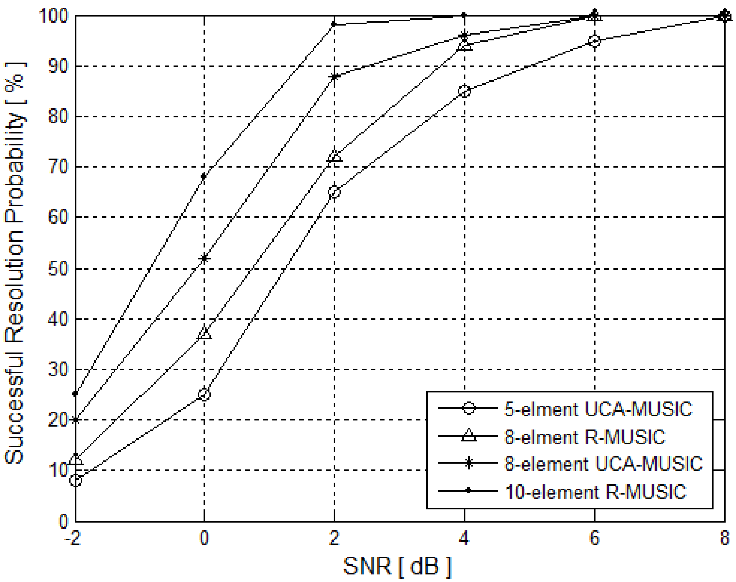
5.1.2. The Resolution Probability versus SNR

Two signal DOAs are (90°, 81°) and (90°, 85°), respectively, and both the signal frequencies are 6 GHz. Figure 4 displays the resolution probability of the eight-element R-MUSIC, 10-element R-MUSIC, five-element UCA MUSIC, and eight-element UCA MUSIC versus the SNR from −2 to 8 dB with snapshots number L = 100. While Figure 5 displays the resolution probability of the four methods versus the snapshots number from 16 to 144 with SNR = 20 dB. Every data is averaged over 200 Monte Carlo simulations. It can be seen from Figure 4 and Figure 5 that the resolution performance of the proposed eight-element R-MUSIC is close to that of the five-element UCA-MUSIC, but the successful probability is lower than that of the eight-element UCA-MUSIC. However, if we select 10 elements to form a UCA, then the resolution performance will be better than that of the eight-element UCA-MUSIC.

Figure 3. Spatial spectrum with multiple signals. (a) Two signal DOAs are (90°, 70°) and (90°, 80°); (b) Three DOAs are (60°, 30°), ( 90°, 60°) and ( 120°, 80°); (c) Four DOAs are (60°, 40°), (90°, 80°), (120°, 60°) and (140°, 40°).

Figure 4. Successful resolution probability versus SNR.

Figure 5. Successful resolution probability versus snapshots number.

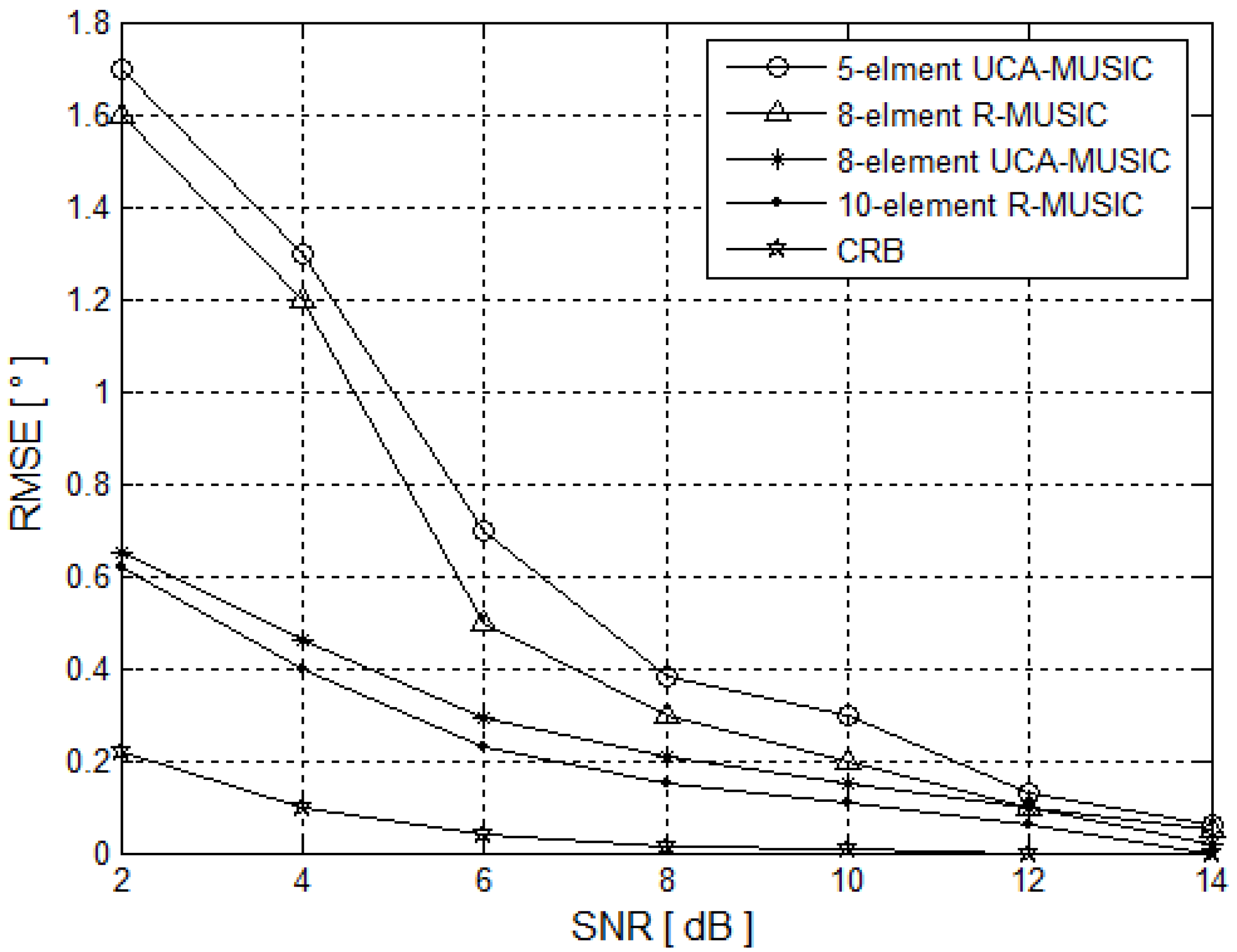
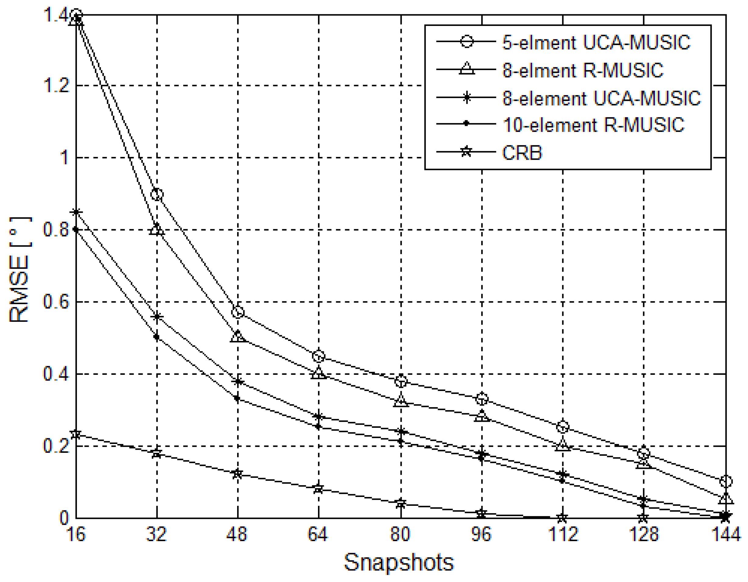
5.2. Estimation Accuracy Performance Simulation

Two signal DOAs are (90°, 81°) and (90°, 85°), respectively, both the signal frequencies are 6 GHz. Figure 6 displays the root mean square error (RMSE) of the eight-element R-MUSIC, 10-element R-MUSIC, five-element UCA MUSIC, and eight-element UCA MUSIC versus the SNR from 2 to 14 dB with snapshots L = 100. While Figure 7 displays the resolution probability of the four methods versus the snapshots from 16 to 144 with SNR = 10 dB. Every data is averaged over 200 Monte Carlo simulations. It can be seen from Figure 6 and Figure 7 that the RMSE of the proposed algorithm approximates to the CRB and the RMSE of the four methods is decreasing with increasing snapshots. Besides, the estimation accuracy performance of the proposed eight-element R-MUSIC is better than that of the five-element UCA-MUSIC, but which is lower than that of the eight-element UCA-MUSIC. However, the estimation accuracy of the 10-element R-MUSIC is better than that of the eight-element UCA-MUSIC.

Figure 6. RMSE versus SNR.

Figure 7. RMSE versus snapshots.

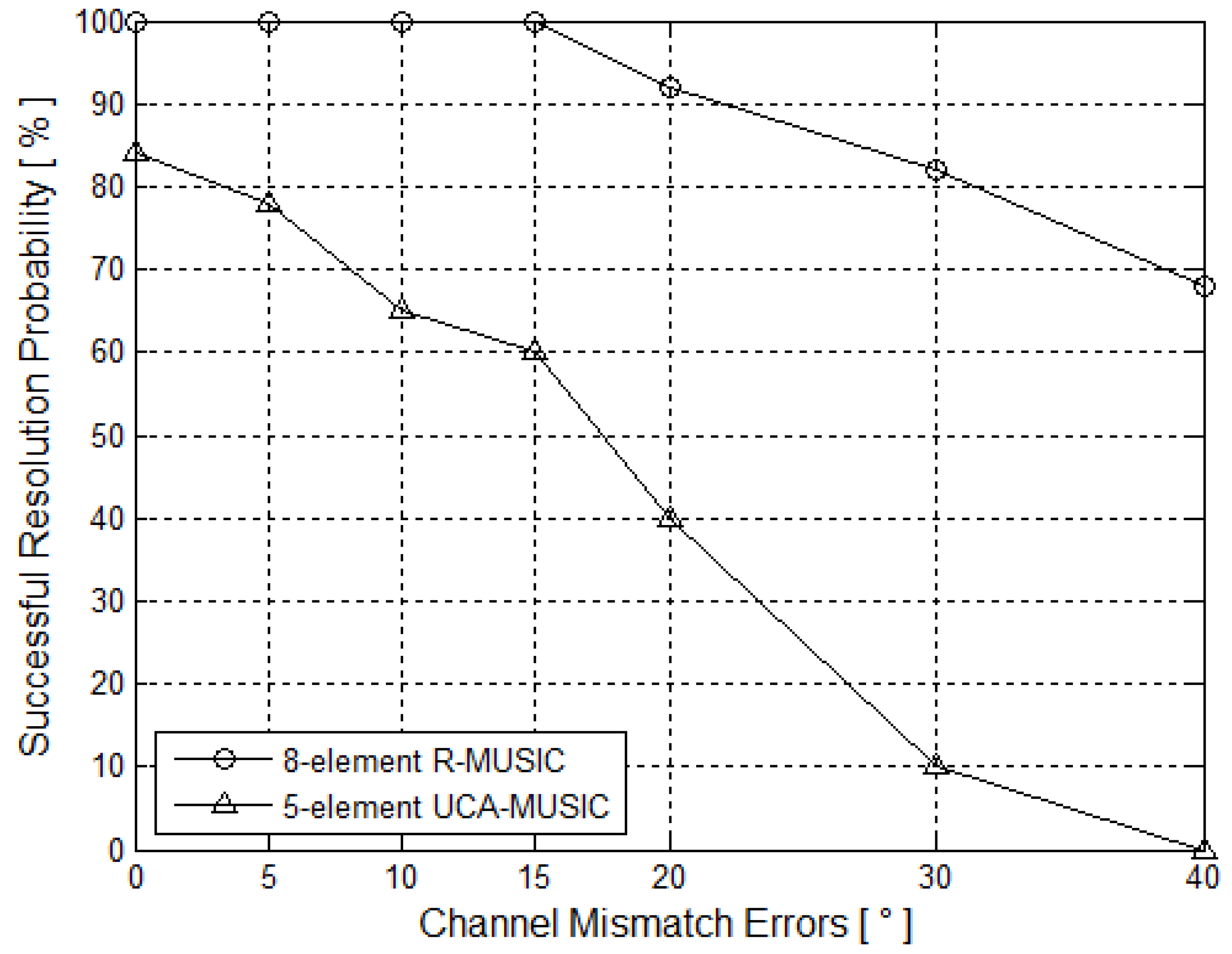
5.3. Channel Mismatch Errors Simulation

The influence of channel mismatch errors on the resolution probability of the eight-element R-MUSIC and five-element MUSIC is shown in Figure 8. The channel mismatch errors range from 0 to 40°, SNR is 6 dB and the snapshots number is 100. The two DOAs are the same as the simulation in Subsection 5.2. Every data is averaged over 200 Monte Carlo simulations. Table 1 shows the RMSE versus the channel mismatch errors. Because the statistical characteristics of the two DOAs are the same, both Figure 8 and Table 1 shows the estimation results of DOA = (90°, 85°).

It can be seen from the Figure 8 that the proposed R-MUSIC algorithm can provide better robustness than that of the classical MUSIC in large channel mismatch errors. Table 1 shows the estimation accuracy performance of R-MUSIC is much better than that of the classical MUSIC, when the channel mismatch errors exist. This is because the R-MUSIC algorithm only needs two elements; the number of elements of R-MUSIC is much less than that of the classical MUSIC. Furthermore, the problem of element channel calibration is easier to solve too.

Figure 8. Successful resolution probability versus different channel mismatch errors.

Table 1. The RMSE versus different channel mismatch errors [degree]

Channel mismatch errors [degree]	5-elment UCA-MUSIC	8-element R-MUSIC
0	0.1414	0.2739
5	0.2191	0.2162
10	0.4817	0.4000
15	0.5441	0.4427
20	0.6132	0.4336

Table 1. The RMSE versus different channel mismatch errors [degree]

Channel mismatch errors [degree]	5-elment UCA-MUSIC	8-element R-MUSIC
0	0.1414	0.2739
5	0.2191	0.2162
10	0.4817	0.4000
15	0.5441	0.4427
20	0.6132	0.4336

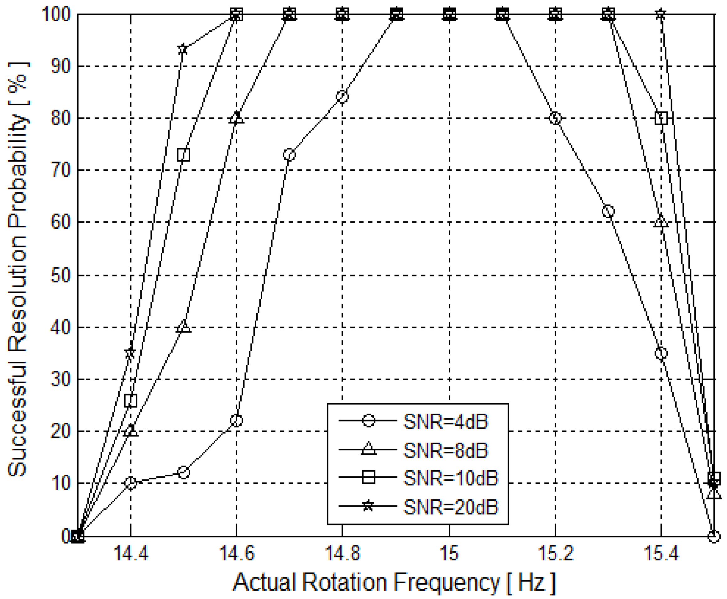
5.4. Resolution Performance versus Rotation Frequency Errors

There are two inherent incident signals with DOAs are (90°, 81°) and (90°, 85°) respectively, both the signal frequencies are 6 GHz. The snapshots number is L = 100, and in theory, the rotation frequency is ƒ_z = 15H_Z. However, in fact, the rotation velocity will be greater or smaller than the theory rotation frequency ƒ_z. Now, assume the actual rotation frequency is ƒʹ, and let ƒʹ range from 14.3 to 15.5 Hz by the step 0.1 Hz in this simulation. So, the rotation frequency error is ∆ƒ = ƒʹ − ƒ_z. shows the successful resolution probability versus rotation frequency error when SNR = 4 dB, 8dB, 10 dB and 20 dB, successively.

As shown in Figure 9, when ƒʹ = ƒ_z and the SNR>8 dB, the successful resolution probability of the R-MUSIC is 100%; However, when the actual rotation frequency ƒʹ is larger or smaller than ƒ_z, the successful resolution probability will decrease. The larger the |∆ƒ| is, the lower the successful resolution probability is. On the other hand, when SNR = 4 dB, the successful rotation frequency (>60%) ranges from 15 − 0.3 ~ 15 + 0.3 Hz; When SNR = 10 dB, the successful rotation frequency ranges from 15−0.4 ~ 15 + 0.4 Hz; When SNR = 20 dB, the successful rotation frequency ranges from 15 − 0.5 ~ 15 + 0.4 Hz; that is to say, with increases in SNR, the rotation array system can tolerate wider rotation frequency error range. However, when ∆ƒ is larger than a certain value, even increasing SNR would not improve resolution. That is because according to Equation (15), a larger rotation frequency error will cause a Doppler frequency shift, which has a great influence on the estimation and resolution performance of the proposed algorithm.

Figure 9. Successful resolution probability versus rotation frequency errors.

6. Conclusions

The performance of classical MUSIC algorithm based on UCA is constrained by array aperture greatly, and most DOA estimation algorithms demand that the number of elements be larger than that of incident signals. Focusing on this problem, a novel multiple DOAs estimation algorithm based on rotation array is proposed in this paper, which has lower energy loss and complexity. Computer simulations verify the effectiveness of the proposed method, and the number of incident signals that the algorithm could estimate is more than that of the elements. Besides, the proposed array model could be used for any algorithm based on UCA. In the future work, we will focus on the application of the proposed algorithm [25].

References

- Schmidt, R.O. Multiple Emitter location and signal parameter estimation. IEEE Trans. Antennas Propag. 1986, 34, 276–280. [Google Scholar] [CrossRef]
- Rubsamen, M.; Gershman, A.B. Direction of arrival estimation for nonuniform sensor arrays: From manifold separation to Fourier domain MUSIC methods. IEEE Trans. Signal Process. 2009, 57, 588–599. [Google Scholar] [CrossRef]
- Gao, F.F.; Nallanathan, A.; Wang, Y.D. Improvd MUSIC under the coexistence of both circular and noncircular sources. IEEE Trans. Signal Process. 2008, 56, 3033–3038. [Google Scholar] [CrossRef]
- You, H.; Huang, J.G.; Jin, Y. Improving MUSIC performance in snapshot deficient scenario via weighted signal-subspace projection. Syst. Eng. Electron. 2008, 30, 792–794. [Google Scholar]
- Mestre, X.; Lagunas, M. Modified subspace algorithms for DOA estimation with large arrays. IEEE Trans. Signal Process. 2008, 56, 598–614. [Google Scholar] [CrossRef]
- Mccloud, M.L.; Scharf, L.L. A new subspace identification algorithm for high-resolution DOA estimation. IEEE Trans. Antennas Propag. 2002, 50, 1382–1390. [Google Scholar] [CrossRef]
- Liu, J.; Yu, H.Q.; Huang, Z.T. Conjugate extended MUSIC algorithm based on second-order preprocessing. Syst. Eng. Electron. 2008, 30, 57–60. [Google Scholar]
- Liu, H.S.; Xiao, X.C. An approach to designing linear array with high accuracy doa estimate based on minimal manifold length. Acta Aeronaut. Etastronautica Sin. 2008, 29, 462–466. [Google Scholar]
- He, M.H.; Yin, Y.X.; Zhang, X.D. UCA-ESPRIT algorithm for 2-D angle estimation. IEEE Trans. Signal Process. 2000, 1, 437–440. [Google Scholar]
- Goosens, R.; Rogier, H.; Werbrouck, S. UCA Root-MUSIC with sparse uniform circular arrays. IEEE Trans. Signal Process. 2008, 56, 4095–4099. [Google Scholar] [CrossRef]
- Wu, Y.T.; So, H.C. Simple and accurate two-dimensional angle estimation for a single source with uniform circular array. IEEE Antennas Wirel. Propag. Lett. 2008, 7, 78–80. [Google Scholar] [CrossRef]
- Pajsusco, P.; Pagani, P. On the use of uniform circular array for characterizing UWB time reversal. IEEE Trans. Antennas Propag. 2009, 57, 102–109. [Google Scholar] [CrossRef]
- Huang, L.; Wu, S.; Feng, D. Low complexity method for signal subspace filtering. IEEE Electron. Lett. 2004, 40, 34–38. [Google Scholar] [CrossRef]
- Goosens, R.; Rogier, H. A hybrid UCA RARE or root MUSIC approach of 2D direction of arrival estimation in uniform circular arrays in the presence of mutual coupling. IEEE Trans. Antennas Propag. 2007, 55, 841–849. [Google Scholar] [CrossRef]
- Tao, J.W.; Shi, Y.W.; Chang, W.X. The estimation of 2-D DOA of scattered sources with UCAs. J. China Inst. Commun. 2003, 24, 10–17. [Google Scholar]
- Tao, J.W.; Shi, Y.W.; Chang, W.X. Cross correlation estimator of azimuth-elevation with UCAs. Acta Electron. Sin. 2003, 31, 575–575. [Google Scholar]
- Tang, Z.L.; Wu, S.J.; Zhang, S. Estimation of 2-D DOA based on uniform circle array. J. Harbin Eng. Univ. 2005, 26, 247–252. [Google Scholar]
- Xu, D.C.; Liu, Z.W.; Qi, X.D. A unitary transformation method for DOA estimation with uniform circular array. Radio Eng. 2010, 40, 13–16. [Google Scholar]
- Lu, L.Q.; Hu, X.P.; Wu, M.P. Fast orientation determination by Twin-Star system through method of rotating baseline. J. Astronaut. 2004, 25, 158–162. [Google Scholar]
- Si, W.J.; Cheng, W. Study on solving ambiguity Method of rolling interferometer and implemention. J. Proj. Rocket. Missiles Guid. 2010, 30, 199–202. [Google Scholar]
- Yaqoob, M.A.; Tufvesson, F.; Mannesson, A.; Bernhardsson, B. Direction of arrival estimation with arbitrary virtual antenna arrays using low cost inertial measurement units. In Proceedings of the IEEE ICC 2013 Workshop on Advances in Network Localization and Navigation, Budapest, Hungary, 9–13 June 2013.
- de Jong, Y.L.C.; Herben, M.H.A.J. High-resolution angle-of arrival measurement of the mobile radio channel. IEEE Trans. Antennas Propag. 1999, 47, 1677–1687. [Google Scholar] [CrossRef]
- Broumandan, A.; Lin, T.; Moghaddam, A. Direction of Arrival Estimation of GNSS Signals Based on Synthetic Antenna Array. In Proceedings of the International Technical Meeting (ION GNSS 2007), Fort Worth, TX, USA, 25–28 September 2007.
- Yuan, X.H.; Zhen, H.; Yu, F.Q. Cramer-Rao bound for 2-D angle estimation with uniform circular array. J. Telecommun. Eng. 2013, 53, 44–51. [Google Scholar]
- Han, G.J.; Xu, H.; Duong, T.Q.; Jiang, J.; Takahiro, H. Localization algorithms of wireless sensor networks: A survey. Telecommun. Syst. 2013, 52, 2419–2436. [Google Scholar] [CrossRef]
© 2014 by the authors; licensee MDPI, Basel, Switzerland. This article is an open access article distributed under the terms and conditions of the Creative Commons Attribution license (http://creativecommons.org/licenses/by/3.0/).