Understanding Differential Privacy in Decentralized Federated Learning: A Controlled Privacy–Utility Comparison

Abstract

Centralized Federated Learning (FL) enables collaborative model training without sharing raw data. Differential privacy (DP) is widely used to protect sensitive information in FL; however, its behavior in decentralized environments remains poorly understood. This study empirically compares centralized FL and sequential Decentralized Federated Learning (DFL) under matched clipping and perturbation settings to examine model utility and privacy leakage. Both frameworks were evaluated under a common experimental setup with non-IID data, and each configuration was evaluated across five independent seeds. Utility was evaluated under matched experimental perturbation parameters, whereas formal client-level privacy accounting was applied to the perturbed round-end model releases, with each client’s complete dataset treated as the protected unit. Empirical leakage was evaluated separately using membership inference and gradient inversion attacks. Within the evaluated MNIST configuration, the results show that clipping, perturbation, and the learning procedure jointly influence the observed privacy–utility behavior. At $C=1$ and ${ϵ}_{\mathrm{cal}}=2$, the mean final accuracy was $73.83\%$ for FL and $97.74\%$ for sequential DFL. At ${ϵ}_{\mathrm{cal}}=4$, InvGrad reconstruction for FL produced an MSE of $0.048$, PSNR of $13.71$, and SSIM of $0.280$, compared with $0.130$, $10.10$, and $0.184$ for sequential DFL, respectively. Future research will investigate topology-aware privacy mechanisms and adaptive noise allocation for decentralized systems.

1. Introduction

Machine learning systems are increasingly trained on data from multiple sources. Privacy concerns may prevent collecting these data in a single location [1]. Federated Learning (FL) is a distributed learning strategy that lets users collaboratively train a shared model without exchanging raw data [2]. Since its introduction, FL has been adopted across many domains, including healthcare [3], finance [4], and mobile applications [5]. Conventional FL relies on a central server to coordinate training and aggregate model updates. This approach has several drawbacks, including communication bottlenecks and a single point of failure [6].

Decentralized Federated Learning (DFL) has emerged as an alternative strategy to address these problems. In DFL, participating nodes exchange model updates directly without relying on a central coordinator [7]. However, this design also introduces new challenges, including potentially slower convergence, increased communication complexity, and greater sensitivity to communication topology and update propagation behavior [8]. Recent work has examined the optimization and communication characteristics of centralized and decentralized FL [9,10,11,12], but privacy remains a major challenge in both settings. Model updates can still reveal sensitive information about participating users, even when raw training data are not shared [13]. Adversaries can use shared updates to reconstruct data or infer information about training samples.

Differential privacy (DP) provides a formal approach for limiting information leakage by introducing controlled randomization into the learning process [14]. In iterative learning, privacy loss accumulates across repeated releases, making privacy accounting an important part of the evaluation. Rényi differential privacy (RDP) provides a convenient framework for composing privacy loss across multiple mechanisms and converting the accumulated loss to an $(ϵ,\delta )$-DP guarantee [15]. The behavior of DP has been widely studied in centralized FL systems. Previous work has examined the relationship between privacy protection and model utility under different configurations [16,17,18,19].

DP behavior in decentralized environments remains insufficiently explored [20]. DFL relies on sequential or peer-to-peer information exchange, causing updates to propagate differently through the network. Recent studies [21,22] have shown that network structure and distributed communication patterns can affect privacy behavior. However, empirical evidence comparing centralized FL and decentralized learning under matched perturbation and clipping settings remains limited. In particular, the interaction between the learning procedure, clipping, model utility, formal privacy accounting, and empirical privacy leakage requires further investigation.

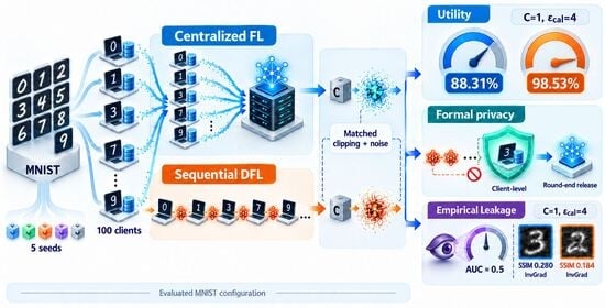
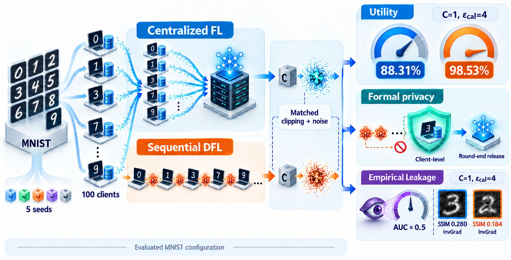
To address this gap, this study empirically compares centralized FL and sequential DFL using non-IID data. The privacy–utility trade-off is examined from multiple perspectives rather than through a single measure. Model utility is evaluated through learning performance, convergence, utility retention, accuracy degradation, and clipping behavior. Formal privacy is evaluated through RDP accounting, while empirical leakage is examined using Membership Inference Attacks (MIAs) and gradient inversion attacks.

Comparisons under matched experimental perturbation parameters, formal privacy guarantees, and empirical privacy leakage are treated as distinct analyses. The formal guarantees are interpreted under the stated adjacency, protected-unit, and release assumptions.

The study has the following objectives:

• Evaluate model utility in centralized FL and sequential DFL under different clipping and DP-related perturbation settings.
• Examine how the learning procedure influences the response to clipping and perturbation during collaborative model training.
• Compare utility retention and accuracy degradation relative to the corresponding No-DP baselines.
• Evaluate privacy leakage using Membership Inference Attacks and gradient inversion attacks.
• Describe the relationship between the learning procedure, privacy-related perturbations, and model utility in the evaluated FL and sequential DFL settings.

This study is intended for researchers and practitioners working on federated learning, decentralized learning, and privacy-preserving machine learning. The comparison helps readers understand how the same perturbation settings can affect centralized and decentralized learning differently. It also shows why privacy and utility results should be interpreted in the context of the learning protocol and its communication structure. These findings can support the design and evaluation of privacy-preserving distributed learning systems.

The rest of the paper is organized as follows. Section 2 reviews related work. Section 3 describes the methodology and experimental setup. Section 4 presents the experimental results. Section 5 discusses the results and highlights the main findings. Finally, Section 6 concludes the paper and discusses future research directions.

2. Related Work

FL has become a well-known option for privacy-preserving distributed learning. DP is also one of the most commonly used methods for safeguarding confidential data during cooperative training. This section examines research on centralized and decentralized FL and the use of DP in both contexts. It then reviews current comparative studies and identifies the research gap this work aims to fill.

2.1. Centralized Federated Learning

Research on distributed learning systems has mostly concentrated on improving robustness, communication efficiency, and optimization. McMahan et al.’s Federated Averaging (FedAvg) approach [23] laid the foundation for contemporary FL. FL has since become one of the most widely used techniques for distributed machine learning. FL faces a major difficulty due to statistical variance in participant counts. In real-world implementations, data are not identically distributed (non-IID), which slows down global convergence and causes local model updates to stray. Many prior studies have addressed this issue. For example, Zhao et al. [24] showed how non-IID data affects federated optimization. MOON improves consistency between local and global representations using model-contrastive learning [25]. FedProx employs a proximal regularization term to control excessive discrepancy between local and global models during optimization [26]. These techniques aim to improve convergence and reduce client drift without altering the core aggregation mechanism. FL has also received considerable attention for communication efficiency. Large-scale FL can create communication bottlenecks. Researchers have proposed numerous solutions to reduce communication overhead and maintain learning effectiveness. These solutions include resource-aware optimization methods, adaptive client-involvement mechanisms, and communication-efficient training approaches [27,28,29].

2.2. Decentralized Federated Learning

Decentralized FL aims to eliminate the single point of failure and improve system resilience [7]. This structural modification further complicates communication and optimization by changing how knowledge spreads throughout the learning process. Among the oldest and most important techniques is the Decentralized Parallel Stochastic Gradient Descent (D-PSGD) [30]. This structure uses a peer-to-peer model for sharing and decentralized averaging. More recently, random walks have been proposed to reduce communication overhead and enhance performance [31]. The random walk protocol propagates models sequentially among nodes. Many factors can affect the behavior of decentralized systems, including network design, connectivity patterns, peer selection methods, and information dissemination pathways. Recent studies on topology-aware optimization methods seek to improve learning performance in decentralized settings [11,12]. Extensive surveys have raised several unanswered questions, including sensitivity to varying data distributions, convergence stability, and communication complexity [7,8]. Privacy and security remain critical because participating nodes still need to share model updates during learning. Privacy safeguards may operate differently from those used in traditional FL. Understanding these differences has become increasingly crucial as distributed learning evolves and is therefore a research focus.

2.3. Differential Privacy in Federated and Decentralized Learning

DP offers quantitative privacy guarantees [32]. Researchers frequently apply gradient clipping and noise injection to achieve DP in centralized FL [33]. Later studies have applied this method in federated settings by incorporating resilience mechanisms and adaptive privacy settings [34,35,36]. Overall, these studies show that DP can effectively mitigate privacy risks and reduce data leakage. Using DP in distributed systems presents new challenges [37]. Because Decentralized FL lacks a central organizer like standard FL, it needs privacy safeguards to operate across distributed communication channels. Therefore, network topology and how information propagates among nodes can affect privacy assurances [38]. Recently, research has started on privacy-preserving techniques for decentralized environments. Rodio et al. [39] developed a correlated-noise approach to improve the privacy–utility trade-off by spreading privacy protection across distributed learning processes. Ghazi et al. [21] theoretically proposed DP on Trust Graphs, thereby demonstrating how participant confidence relationships and graph structure may influence privacy guarantees. Emphasizing the increasing relevance of topology-aware privacy models, Mueller et al. [22] investigated machine learning and privacy-preserving analytics in graph-based systems. A recent review of privacy-preserving methods in DFL also showed that many current methods are still in the early stages of development. Unaddressed problems persist in decentralized optimization, communication dynamics, and privacy accounting [20]. Although these studies offer important insights into combining DP across centralized and distributed learning approaches, most recent work examines each environment separately. Therefore, it remains unknown how decentralization affects the privacy–utility trade-off and whether DP behaves differently in centralized versus decentralized learning environments. To address this question, controlled experimental investigations are needed to isolate the influence of the learning design while maintaining consistent testing conditions and privacy protections.

2.4. Comparative Studies Between Centralized and Decentralized Learning

Many studies have compared centralized and decentralized learning. These studies mainly examined performance, convergence behavior, scalability, robustness, and application-specific results. For predictive main maintenance, Kamei and Taghipour [40] conducted an experimental comparison and showed that under certain conditions, decentralized approaches could match the performance of centralized approaches. Chongder [41] studied several federated aggregation techniques and found that decentralized aggregation offers comparable performance while reducing reliance on centralized management. These efforts help us better grasp distributed learning setups, even though they mostly focus on expected results and system behavior. Sun et al. [42] conduct a theoretical investigation of variations in stability and generalization between the two learning frameworks. Their findings suggest that network architecture and communication methods could affect learning processes. Similarly, Li et al. [43] argued that the underlying optimization and communication processes distinguish centralized from decentralized learning. These results suggest that architectural design choices may affect several facets of the learning process, including robustness, utility, and possibly privacy. Findings from Diniz et al. [44] on healthcare applications suggest that decentralized methods may improve performance and data governance. Although this study analyzes the viability of decentralized learning, it focuses on application-level efficiency rather than privacy-preserving technologies. To clarify the comparison,

Table 1. Summary of comparative studies on centralized and decentralized learning.

Study	Main Outcome	Limitation/Research Gap
Kamei and Taghipour [40]	Decentralized approaches can achieve performance comparable to centralized approaches under the studied conditions.	The study focuses mainly on predictive performance and does not examine DP-based privacy.
Chongder [41]	Decentralized aggregation can provide comparable performance while reducing reliance on centralized management.	The comparison focuses on aggregation and performance rather than the effect of DP.
Sun et al. [42]	Network structure and communication methods can affect stability and generalization.	The study is mainly theoretical and does not empirically compare DP behavior.
Li et al. [43]	Centralized and decentralized learning differ in optimization, communication, privacy, and robustness.	The work provides theoretical insights but does not empirically compare the effect of DP across both settings.
Diniz et al. [44]	Decentralized learning can improve performance and data governance in healthcare applications.	The study focuses on application-level performance rather than DP-based privacy.

summarizes the main outcomes and identifies the key limitations and research gaps relevant to this study.

Table 1 shows that existing comparisons mainly focus on performance, convergence, aggregation, stability, or application-specific behavior. The effect of DP across centralized and decentralized learning remains less explored. In particular, empirical evidence on how FL and DFL respond to matched perturbation and clipping settings remains limited. Few studies jointly examine model utility, formal privacy guarantees, and empirical privacy leakage through a controlled comparison.

This study addresses this gap by comparing centralized FL and sequential DFL under matched experimental settings. The matched-perturbation comparison, formal privacy analysis, and empirical leakage evaluation are reported separately. The evaluation is limited to the centralized FL and sequential DFL implementations considered in this study and is not intended as a benchmark against existing DP-DFL methods.

3. Methodology

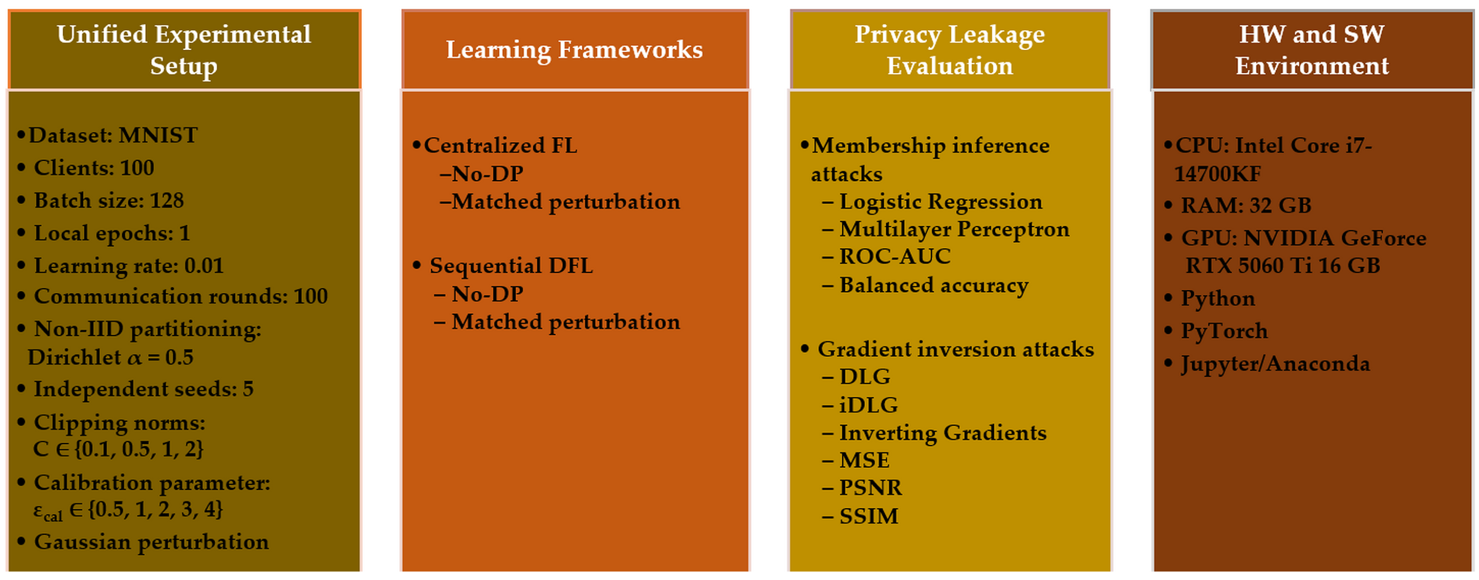
This study uses a unified experimental framework to compare centralized FL and sequential DFL in terms of learning performance, formal privacy accounting, and empirical privacy leakage. The overall methodology is summarized in Figure 1.

As shown in Figure 1, the methodology covers the unified experimental setup, the FL and sequential DFL learning configurations, privacy definition and accounting, privacy leakage evaluation, and the hardware and software environment. The following subsections describe these components.

3.1. Unified Experimental Setup

The experiments used the MNIST benchmark dataset [45], which consists of 60,000 training images from 10 handwritten-digit classes. Each image is a single-channel $28\times 28$ grayscale image. The images were converted to tensors and normalized using a mean of 0.1307 and a standard deviation of 0.3081.

All experiments were repeated across five independent seeds. For each experimental seed, the 60,000 samples were divided into four non-overlapping subsets using stratified sampling: 40,000 samples for target-model training, 5000 for target-model holdout evaluation, 10,000 for shadow-model training, and 5000 for shadow-model holdout evaluation. The target-training subset was distributed among 100 clients using a Dirichlet distribution with concentration parameter $\alpha =0.5$ to produce a non-IID client partition.

Both frameworks were trained for 100 communication rounds. Local optimization used stochastic gradient descent (SGD) with one local epoch per client participation, a batch size of 128, a learning rate of 0.01, momentum of 0.9, and weight decay of $5\times {10}^{-4}$. Gradient clipping with a maximum norm of 10 was applied during local optimization.

A lightweight convolutional neural network (CNN) was used for image classification. The network contains two convolutional layers with 16 and 32 output channels, respectively, using $3\times 3$ kernels with padding of 1. Each convolutional layer is followed by a ReLU activation and max pooling. The network then uses a fully connected layer with 128 ReLU units, dropout with a probability of 0.2, and a 10-unit output layer.

The matched-perturbation experiments considered ${ϵ}_{\mathrm{cal}}\in \{0.5,1,2,3,4\}$ and clipping norms $C\in \{0.1,0.5,1,2\}$. For an update vector u, ${\mathcal{l}}_2$ clipping is defined as

$$\overline{u}=u·\min \left(1,{\displaystyle \frac{C}{{\parallel u\parallel }_2}}\right).$$

(1)

Gaussian perturbation was subsequently applied to the clipped update. For each $(C,{ϵ}_{\mathrm{cal}})$ condition, the same absolute perturbation scale was used for FL and sequential DFL. This matching supports a controlled perturbation comparison but does not imply equal formal privacy guarantees. The parameter ${ϵ}_{\mathrm{cal}}$ determines the perturbation scale and does not represent the achieved cumulative privacy budget.

A No-DP baseline was also evaluated for each framework without model-update clipping or Gaussian perturbation. Optimizer-level gradient clipping with a maximum norm of 10 was retained in all conditions as part of the common optimization configuration.

The same data splits, client partitions, model architecture, training hyperparameters, and experimental seeds were used for FL and sequential DFL. The frameworks differed in their aggregation and model-propagation procedures, as described in the following subsection.

3.2. Learning Frameworks and Experimental Scenarios

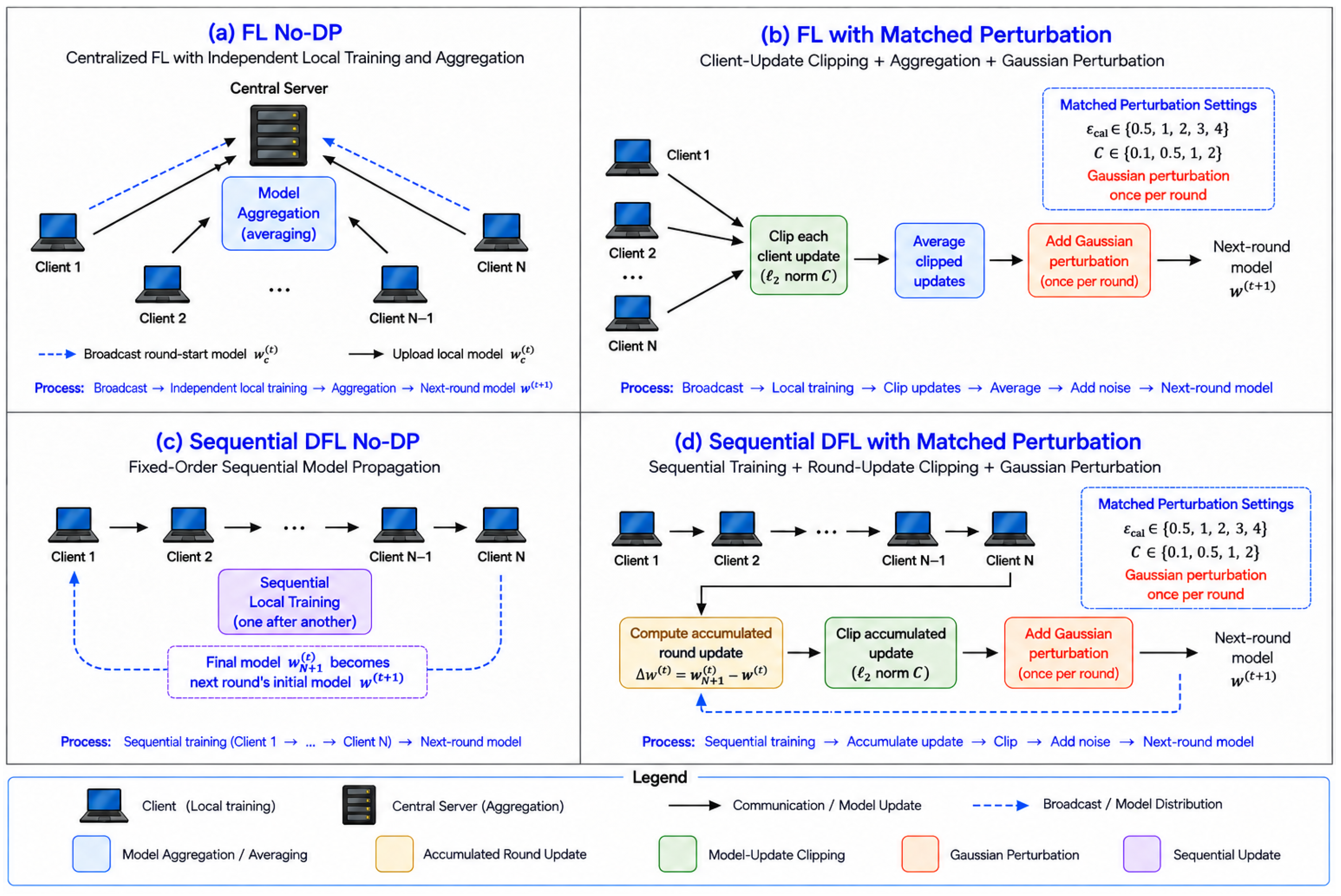
Four experimental scenarios were evaluated by combining centralized FL and sequential DFL with No-DP and matched-perturbation conditions. Let $N=100$ denote the number of participating clients, $w^{\left(t\right)}\in {\mathbb{R}}^d$ denote the model parameters at the beginning of communication round t, and ${\mathcal{D}}_i$ denote the local dataset of client i. Figure 2 illustrates the four configurations.

The centralized configurations aggregate client updates that are trained independently. In contrast, the sequential DFL configurations propagate a single model through the clients in a fixed order. The four configurations are described below.

3.2.1. FL No-DP

In the No-DP centralized FL configuration, local training and global aggregation follow the FedAvg framework [23]. At communication round t, all clients initialize their local models from the round-start model $w^{\left(t\right)}$ and perform local training:

$$w_i^{\left(t\right)}=\mathrm{LocalTrain}\left(w^{\left(t\right)},{\mathcal{D}}_i\right),i=1,\dots ,N.$$

(2)

The resulting client models are averaged to obtain

$$w^{(t+1)}={\displaystyle \frac{1}{N}}{\displaystyle \sum _{i=1}^N}{w}_i^{\left(t\right)}.$$

(3)

No model-update clipping or Gaussian perturbation is applied in this configuration.

3.2.2. FL with Matched Perturbation

In the matched-perturbation FL configuration, each client independently trains a local model initialized from $w^{\left(t\right)}$ and computes

$$\Delta w_i^{\left(t\right)}=w_i^{\left(t\right)}-w^{\left(t\right)}.$$

(4)

Each update is clipped to the ${\mathcal{l}}_2$ threshold C [33]:

$${\overline{\Delta w}}_i^{\left(t\right)}=\Delta w_i^{\left(t\right)}\min \left(1,{\displaystyle \frac{C}{\parallel \Delta w_i^{\left(t\right)}{\parallel }_2}}\right).$$

(5)

The clipped updates are averaged as

$${\overline{\Delta w}}^{\left(t\right)}={\displaystyle \frac{1}{N}}{\displaystyle \sum _{i=1}^N}{\overline{\Delta w}}_i^{\left(t\right)}.$$

(6)

Gaussian perturbation is then applied once per communication round:

$$w^{(t+1)}=w^{\left(t\right)}+{\overline{\Delta w}}^{\left(t\right)}+z^{\left(t\right)},z^{\left(t\right)}\sim \mathcal{N}\left(0,{\sigma }_{\mathrm{abs}}^{2}I\right),$$

(7)

where ${\sigma }_{\mathrm{abs}}$ is the absolute Gaussian standard deviation defined in Section 3.3. The complete procedure is summarized in Algorithm 1.

Algorithm 1 Centralized FL with Matched Perturbation

Require: Initial model $w^{\left(0\right)}$, client datasets ${\left\{{\mathcal{D}}_i\right\}}_{i=1}^N$, number of rounds T, local epochs E,   learning rate $\eta$, clipping threshold C, absolute noise standard deviation ${\sigma }_{\mathrm{abs}}$ Ensure: Final model $w^{\left(T\right)}$   1: for $t=0$ to $T-1$ do   2:    Broadcast $w^{\left(t\right)}$ to all clients   3:    for $i=1$ to N do   4:      $w_i\leftarrow$ localtrain$(w^{\left(t\right)},{\mathcal{D}}_i,E,\eta )$   5:      $\Delta w_i\leftarrow w_i-w^{\left(t\right)}$   6:      ${\overline{\Delta w}}_i\leftarrow \Delta w_i\min \left(1,{\displaystyle \frac{C}{\parallel \Delta w_i{\parallel }_2}}\right)$   7:      Send ${\overline{\Delta w}}_i$ to the server   8:    end for   9:    $\overline{\Delta w}\leftarrow {\displaystyle \frac{1}{N}}{\sum }_{i=1}^N{\overline{\Delta w}}_i$ 10:    Sample $z\sim \mathcal{N}(0,{\sigma }_{\mathrm{abs}}^{2}I)$ 11:    $w^{(t+1)}\leftarrow w^{\left(t\right)}+\overline{\Delta w}+z$ 12: end for 13: return  $w^{\left(T\right)}$

3.2.3. Sequential DFL No-DP

In the No-DP sequential DFL configuration, a single model is propagated through all clients in a fixed order. At the beginning of communication round t,

$$w_1^{\left(t\right)}=w^{\left(t\right)}.$$

(8)

Each client performs local training on the model received from its predecessor:

$$w_{i+1}^{\left(t\right)}=\mathrm{LocalTrain}\left(w_i^{\left(t\right)},{\mathcal{D}}_i\right),i=1,\dots ,N.$$

(9)

After all clients have participated, the final model becomes the starting model for the next communication round:

$$w^{(t+1)}=w_{N+1}^{\left(t\right)}.$$

(10)

No model-update clipping or Gaussian perturbation is applied in this configuration.

3.2.4. Sequential DFL with Matched Perturbation

The matched-perturbation sequential DFL configuration uses the fixed client order described above. The model is initialized as

$$w_1^{\left(t\right)}=w^{\left(t\right)},$$

(11)

and is propagated through the clients according to

$$w_{i+1}^{\left(t\right)}=\mathrm{LocalTrain}\left(w_i^{\left(t\right)},{\mathcal{D}}_i\right),i=1,\dots ,N.$$

(12)

After all clients have participated, the accumulated update for the round is

$$\Delta w^{\left(t\right)}=w_{N+1}^{\left(t\right)}-w^{\left(t\right)}.$$

(13)

The accumulated update is clipped once at the end of the round:

$${\overline{\Delta w}}^{\left(t\right)}=\Delta w^{\left(t\right)}\min \left(1,{\displaystyle \frac{C}{\parallel \Delta w^{\left(t\right)}{\parallel }_2}}\right).$$

(14)

Gaussian perturbation is then applied to obtain the model released for the next round:

$$w^{(t+1)}=w^{\left(t\right)}+{\overline{\Delta w}}^{\left(t\right)}+z^{\left(t\right)},z^{\left(t\right)}\sim \mathcal{N}\left(0,{\sigma }_{\mathrm{abs}}^{2}I\right).$$

(15)

The complete procedure is summarized in Algorithm 2.

Algorithm 2 Sequential DFL with Matched Perturbation

Require: Initial model $w^{\left(0\right)}$, client datasets ${\left\{{\mathcal{D}}_i\right\}}_{i=1}^N$, number of rounds T, local epochs E,   learning rate $\eta$, clipping threshold C, absolute noise standard deviation ${\sigma }_{\mathrm{abs}}$ Ensure: Final model $w^{\left(T\right)}$   1: for $t=0$ to $T-1$ do   2:    $v\leftarrow w^{\left(t\right)}$   3:    for $i=1$ to N do   4:      $v\leftarrow$ localtrain$(v,{\mathcal{D}}_i,E,\eta )$   5:      if $i<N$ then   6:         Pass v to client $i+1$   7:      end if   8:    end for   9:    $\Delta w\leftarrow v-w^{\left(t\right)}$ 10:    $\overline{\Delta w}\leftarrow \Delta w\min \left(1,{\displaystyle \frac{C}{{\parallel \Delta w\parallel }_2}}\right)$ 11:    Sample $z\sim \mathcal{N}(0,{\sigma }_{\mathrm{abs}}^{2}I)$ 12:    $w^{(t+1)}\leftarrow w^{\left(t\right)}+\overline{\Delta w}+z$ 13: end for 14: return $w^{\left(T\right)}$

The two frameworks differ in how they incorporate client updates. FL averages independently trained client updates, whereas sequential DFL updates a single model successively across clients. Section 3.3 describes their framework-specific sensitivity and cumulative privacy accounting.

3.3. Threat Model, Privacy Definition, and Accounting

Adversarial access is limited to the perturbed model released at the end of each communication round. For FL, this is the model released after server aggregation and perturbation. For sequential DFL, it is the perturbed model produced after the final client update. Intermediate models exchanged between clients are assumed to be transmitted through protected channels and are excluded from the adversary’s view.

The experiments use ${ϵ}_{\mathrm{cal}}$ to determine the Gaussian perturbation scale. The cumulative privacy guarantee is calculated separately for each framework over the complete training procedure.

The protected unit is a client’s complete dataset. Under client-level replace-one adjacency, two distributed datasets are adjacent if they differ in one client’s dataset while all other client datasets remain unchanged.

For each combination of C and ${ϵ}_{\mathrm{cal}}$, the Gaussian noise standard deviation is determined using the Gaussian mechanism [33,46]:

$${\sigma }_{\mathrm{abs}}={\displaystyle \frac{C}{N}}{\displaystyle \frac{\sqrt{2\ln (1.25/{\delta }_{\mathrm{cal}})}}{{ϵ}_{\mathrm{cal}}}},$$

(16)

where $N=100$ and ${\delta }_{\mathrm{cal}}={10}^{-5}$. The same ${\sigma }_{\mathrm{abs}}$ is used for FL and sequential DFL under each $(C,{ϵ}_{\mathrm{cal}})$ configuration.

In FL, each client update is clipped to an ${\mathcal{l}}_2$ norm of at most C before the N updates are averaged. Under client-level replace-one adjacency, the sensitivity of the released aggregate is bounded by

$${\Delta }_{\mathrm{FL}}\le {\displaystyle \frac{2C}{N}}.$$

(17)

In sequential DFL, the accumulated update is clipped once at the end of each round to an ${\mathcal{l}}_2$ norm of at most C. The sensitivity of the released round-end update is therefore bounded by

$${\Delta }_{\mathrm{DFL}}\le 2C.$$

(18)

Cumulative privacy over the $T=100$ communication rounds was calculated using Rényi differential privacy (RDP) [15]. For a Gaussian mechanism with sensitivity $\Delta$, noise standard deviation ${\sigma }_{\mathrm{abs}}$, and Rényi order $\alpha >1$, the RDP parameter for one release is

$${ϵ}_{\mathrm{RDP}}\left(\alpha \right)={\displaystyle \frac{\alpha }{2}}{\left({\displaystyle \frac{\Delta }{{\sigma }_{\mathrm{abs}}}}\right)}^2.$$

(19)

RDP composes additively across the $T=100$ releases [15], giving

$${ϵ}_{\mathrm{RDP}}^{\left(T\right)}\left(\alpha \right)=T{ϵ}_{\mathrm{RDP}}\left(\alpha \right).$$

(20)

The resulting RDP guarantee was converted to $({ϵ}_{\mathrm{total}},{\delta }_{\mathrm{total}})$ using the standard RDP conversion [15]:

$${ϵ}_{\mathrm{total}}=\underset{\alpha >1}{\min }\left[{ϵ}_{\mathrm{RDP}}^{\left(T\right)}\left(\alpha \right)+{\displaystyle \frac{\ln (1/{\delta }_{\mathrm{total}})}{\alpha -1}}\right],$$

(21)

where ${\delta }_{\mathrm{total}}={10}^{-5}$.

The resulting privacy guarantee applies to the round-end release mechanism and does not extend to intermediate sequential DFL communications.

3.4. Privacy Leakage Evaluation

In addition to the formal privacy analysis, empirical privacy leakage was evaluated using membership inference attacks (MIAs) and gradient inversion attacks (GIAs). These evaluations consider two forms of information exposure: membership disclosure and training-data reconstruction. Because membership inference and gradient reconstruction represent different threat scenarios, each attack was evaluated using a separate experimental configuration. The attack outcomes are analyzed independently of the RDP guarantees. The following subsections describe the two attack methodologies.

3.4.1. Membership Inference Attacks

Membership inference attacks (MIAs) test whether an adversary can distinguish samples used to train a model from samples that were not part of its training set [47]. Following the shadow-model approach of Shokri et al. [48], an attack classifier was trained to distinguish members from non-members using the outputs of a shadow model. The classifier was then applied to the target model.

The attacks were performed for the No-DP baseline and the matched-perturbation conditions at $C=1$ and ${ϵ}_{\mathrm{cal}}\in \{0.5,1,2,3,4\}$ across five independent seeds. For each seed, the MNIST training data were divided into mutually disjoint target and shadow sets using stratified sampling. The target model used 40,000 samples for training and 5000 for holdout evaluation. The shadow model used 10,000 samples for training and 5000 for holdout evaluation. Each shadow model followed the same learning framework and perturbation configuration as its corresponding target model.

The attack classifier was trained on a balanced set of 5000 members from the shadow-training data and 5000 non-members from the shadow holdout set. It was then evaluated on 5000 members from the target-training data and 5000 non-members from the target holdout set. The target and shadow attack data were therefore fully separated.

The MIA adversary was given query access to the final model outputs. For loss-based attacks, the true class labels were also available.

Let $f\left(x\right)$ denote the output logits for input x, with the corresponding class probabilities given by

$$p\left(x\right)=\mathrm{softmax}\left(f\right(x\left)\right).$$

(22)

Three scalar attack features were considered separately: prediction confidence, cross-entropy loss, and prediction entropy. They were defined as

$$c\left(x\right)=\underset{k}{\max }{p}_k\left(x\right),$$

(23)

$$\mathcal{l}\left(x\right)=-\log p_y\left(x\right),$$

(24)

and

$$H\left(x\right)=-{\displaystyle \sum _{k=1}^K}{p}_k\left(x\right)\log \left(p_k\left(x\right)+{10}^{-12}\right),$$

(25)

respectively, where y is the true class label and $K=10$ is the number of classes. The three features were used independently rather than combined into a single feature vector.

Each MIA variant was evaluated using logistic regression (LR) and a multilayer perceptron (MLP). The scalar features were standardized using statistics derived only from the shadow-training data. LR was trained for up to 2000 iterations. The MLP consisted of two hidden layers with 64 and 32 ReLU units. It was trained using Adam with a batch size of 256, a learning rate of ${10}^{-3}$, and a maximum of 300 iterations. Early stopping was applied using 20% of the shadow data for validation.

Each classifier returned a membership probability for every target sample, and ROC-AUC was used as the primary performance metric. Results were computed separately for the five seeds and summarized using the mean and sample standard deviation. We also report 95% confidence intervals based on Student’s t distribution with four degrees of freedom.

3.4.2. Gradient-Leakage Evaluation

Gradient inversion attacks were used to assess whether training samples could be reconstructed from their gradients. Three attacks were evaluated: Deep Leakage from Gradients (DLG) [49], Improved Deep Leakage from Gradients (iDLG) [50], and an Inverting-Gradients-style (InvGrad) attack [51]. The attacks were performed for the No-DP baseline and the matched-perturbation conditions at $C=1$ and ${ϵ}_{\mathrm{cal}}\in \{0.5,1,2,3,4\}$ across five independent seeds.

For each condition, three gradients were examined per seed. For each gradient, a training example was selected from the first local minibatch. Its gradient was computed using the saved model state immediately before the local update. For a training example $(x,y)$ and model parameters w, the observed gradient was

$$g={\nabla }_w\mathcal{L}(w;x,y).$$

(26)

The gradient-inversion adversary was given access to the observed gradient and the corresponding pre-update model state. This attack-specific access is evaluated separately from the round-end release mechanism used for formal privacy accounting.

DLG, iDLG, and InvGrad were applied independently to each gradient. Euclidean gradient matching was used for DLG and iDLG, whereas InvGrad used cosine gradient matching with a total-variation regularization weight of ${10}^{-4}$. Each reconstruction was optimized for 400 iterations using three deterministic restarts. The best result was retained according to the attack objective.

Reconstruction quality was measured using mean squared error (MSE), peak signal-to-noise ratio (PSNR), and structural similarity index (SSIM). The three reconstructions were averaged within each seed. The results were then summarized across the five seeds using the mean, sample standard deviation, and 95% confidence interval based on Student’s t distribution with four degrees of freedom.

3.5. Hardware and Software Configuration

The experiments were conducted on a personal workstation running Windows 11 Pro. The workstation was equipped with an Intel^® Core^™ i7-14700KF processor operating at 3.40 GHz, 32 GB of RAM, and an NVIDIA GeForce RTX 5060 Ti GPU with 16 GB of dedicated memory. The experiments were implemented and executed in an Anaconda Jupyter Notebook environment.

All experiments used Python 3.11.9. The main software libraries included PyTorch 2.12 with CUDA support for model training, NumPy 2.3.5 for numerical computation, Pandas 3.0.1 for data processing and result analysis, Matplotlib 3.10.8 for visualization, and scikit-learn 1.8.0 for membership inference analysis.

Table 2. Experimental configuration used in both frameworks.

Parameter	Configuration
Dataset	MNIST
Original training samples	60,000
Target-model training samples	40,000
Number of clients (N)	100
Data distribution	Non-IID Dirichlet distribution over the target-training subset
Dirichlet parameter ($\alpha$)	0.5
Model architecture	Two-layer CNN with 16 and 32 convolutional channels
Communication rounds (T)	100
Local epochs	1
Batch size	128
Optimizer	Stochastic Gradient Descent (SGD)
Learning rate	0.01
Momentum	0.9
Weight decay	$5\times {10}^{-4}$
Optimizer-level gradient-norm threshold	10
Number of independent seeds	5
Model-update clipping thresholds (C)	$\{0.1,0.5,1,2\}$
Gaussian calibration parameters (${ϵ}_{\mathrm{cal}}$)	$\{0.5,1,2,3,4\}$
Noise-calibration parameter (${\delta }_{\mathrm{cal}}$)	${10}^{-5}$
Privacy-accounting parameter (${\delta }_{\mathrm{total}}$)	${10}^{-5}$
FL communication structure	Centralized FL with equal client-update averaging
DFL communication structure	Fixed-order sequential token passing

summarizes the main experimental configuration used for the FL and sequential DFL experiments.

As summarized in Table 2, both frameworks used the same CNN architecture and training configuration with 100 clients over 100 communication rounds. The data were distributed non-IID using a Dirichlet parameter of $\alpha =0.5$, and each experiment was repeated across five independent seeds. The experiments considered $C\in \{0.1,0.5,1,2\}$ and ${ϵ}_{\mathrm{cal}}\in \{0.5,1,2,3,4\}$. The main difference between the two frameworks was their communication procedure. FL used centralized averaging of client updates, whereas sequential DFL passed the model between clients in a fixed order.

4. Results and Discussion

This section presents the experimental results for the evaluated FL and sequential DFL configurations. The results are organized into separate subsections covering learning performance and convergence efficiency, the impact of DP on model utility, and the outcomes of the privacy attack evaluations.

All results in this section refer to the evaluated MNIST dataset, Dirichlet non-IID configuration with $\alpha =0.5$, CNN architecture, fixed sequential topology, and training settings. Comparisons under matched perturbation parameters do not reflect equal cumulative privacy guarantees.

4.1. Learning Performance and Convergence Efficiency

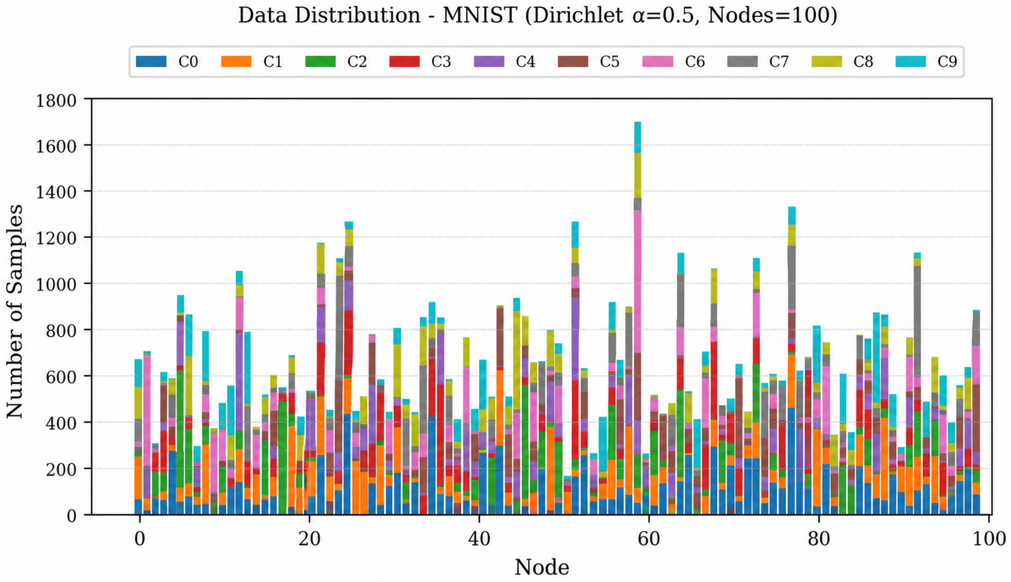
The non-IID distribution of the MNIST training data across the 100 participating clients is shown in Figure 3.

Figure 3 shows the heterogeneous distribution of MNIST classes across the participating clients. Learning performance was evaluated over 100 communication rounds using test accuracy, rounds-to-threshold, and operational stability. The rounds-to-threshold metric is defined as the first communication round at which test accuracy reaches or exceeds 75%. The operational stability round is defined as the first round of a five-consecutive-round window in which the difference between the maximum and minimum test accuracy does not exceed 0.005.

Table 3. Learning performance and convergence results for both frameworks.

Setting	Rounds-to-Threshold		Stability Round		Final Accuracy (%)		Best Accuracy (%)
	FL	DFL	FL	DFL	FL	DFL	FL	DFL
No-DP	$16.20\pm 2.95$	$1.00\pm 0.00$	$42.80\pm 3.49$	$8.80\pm 2.59$	$92.12\pm 0.36$	$98.87\pm 0.12$	$92.14\pm 0.38$	$98.97\pm 0.11$
${ϵ}_{\mathrm{cal}}=0.5$	Not reached (0/5)	Not reached (1/5)	Not reached (2/5)	Not reached (0/5)	$10.23\pm 1.11$	$42.10\pm 22.52$	$25.09\pm 2.72$	$71.70\pm 5.64$
${ϵ}_{\mathrm{cal}}=1$	Not reached (0/5)	$4.80\pm 0.45$	Not reached (0/5)	Not reached (0/5)	$11.97\pm 1.84$	$91.72\pm 3.53$	$36.39\pm 3.52$	$95.49\pm 0.21$
${ϵ}_{\mathrm{cal}}=2$	$50.20\pm 5.89$	$2.00\pm 0.00$	Not reached (1/5)	$25.00\pm 7.45$	$73.83\pm 1.07$	$97.74\pm 0.29$	$77.69\pm 1.96$	$98.02\pm 0.16$
${ϵ}_{\mathrm{cal}}=3$	$25.40\pm 4.45$	$1.80\pm 0.45$	Not reached (2/5)	$14.80\pm 7.05$	$84.73\pm 0.26$	$98.38\pm 0.15$	$86.13\pm 1.09$	$98.56\pm 0.10$
${ϵ}_{\mathrm{cal}}=4$	$21.60\pm 2.19$	$1.60\pm 0.55$	Not reached (3/5)	$9.80\pm 3.11$	$88.31\pm 0.58$	$98.53\pm 0.22$	$88.90\pm 1.02$	$98.76\pm 0.09$

Values are reported as mean ± SD over five independent runs. For rounds-to-threshold and stability, mean ± SD is reported only when all five runs satisfied the corresponding criterion. “Not reached (x/5)” indicates that x of the five runs satisfied the criterion within the 100-round observation horizon.

reports the rounds required to reach the 75% accuracy threshold, the operational stability round, final test accuracy, and best test accuracy for the primary setting $C=1$ and the No-DP baseline. Results are reported as mean ± SD across five independent runs.

Within the evaluated configuration, sequential DFL reached the 75% accuracy threshold in fewer communication rounds than FL whenever both frameworks reached the threshold. Under No-DP, for example, sequential DFL reached the threshold in $1.00\pm 0.00$ rounds, compared with $16.20\pm 2.95$ rounds for FL.

Differences were also observed in final test accuracy. At ${ϵ}_{\mathrm{cal}}=2$, sequential DFL achieved a final accuracy of $97.74\pm 0.29\%$, compared with $73.83\pm 1.07\%$ for FL.

At ${ϵ}_{\mathrm{cal}}=3$, sequential DFL satisfied the operational stability criterion in all five runs, with a mean stability round of $14.80\pm 7.05$. In comparison, only two of the five FL runs satisfied the criterion within the 100-round observation period.

For the settings that showed limited progress within the 100-round evaluation period, the $C=1$ experiments at ${ϵ}_{\mathrm{cal}}\in \{0.5,1\}$ were extended to 200 rounds. The extended results are provided in Appendix A.

4.2. Impact of Matched Perturbation on Model Utility

The effect of the matched perturbation settings on model utility was evaluated relative to the corresponding No-DP baseline of each framework across $C\in \{0.1,0.5,1,2\}$. Utility was assessed using final test accuracy, utility retention, and accuracy degradation based on the mean final test accuracy across five independent runs.

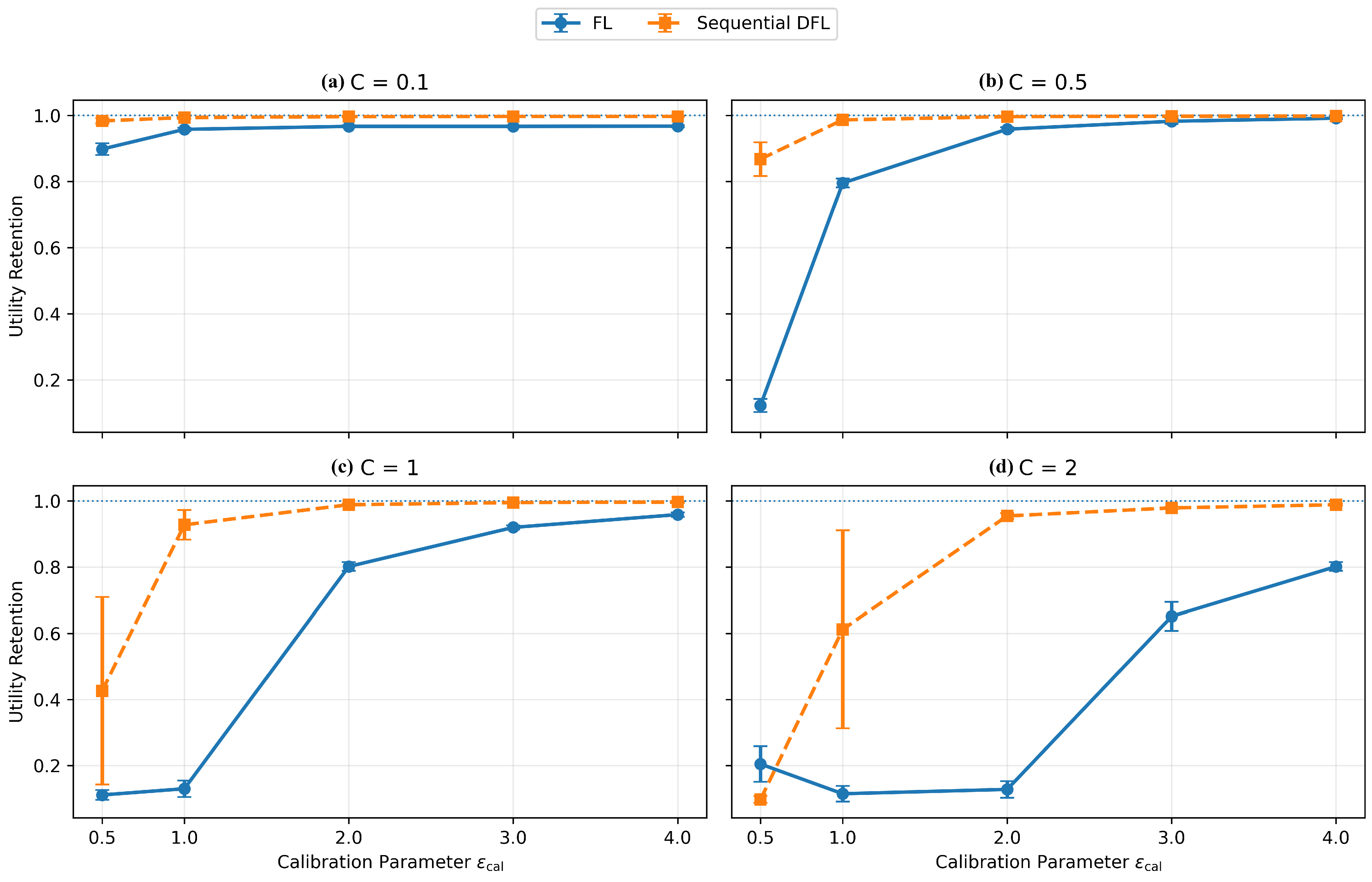
Utility retention was calculated separately for each seed as the ratio of final test accuracy under each matched perturbation setting to the corresponding No-DP final test accuracy. The seed-level values were then summarized across the five independent runs. Figure 4 presents the mean utility retention across the four clipping norms, with error bars indicating 95% confidence intervals.

As shown in Figure 4, utility retention varied across the clipping norms and perturbation settings. At $C=0.1$, retention remained above 89% for FL and 98% for sequential DFL across all evaluated ${ϵ}_{\mathrm{cal}}$ values. At $C=1$ and ${ϵ}_{\mathrm{cal}}=0.5$, retention was approximately 11% for FL and 43% for sequential DFL. At $C=2$, the corresponding values were approximately 20% and 10%, respectively. Greater between-run variability was observed for some settings, particularly for sequential DFL at lower ${ϵ}_{\mathrm{cal}}$ values.

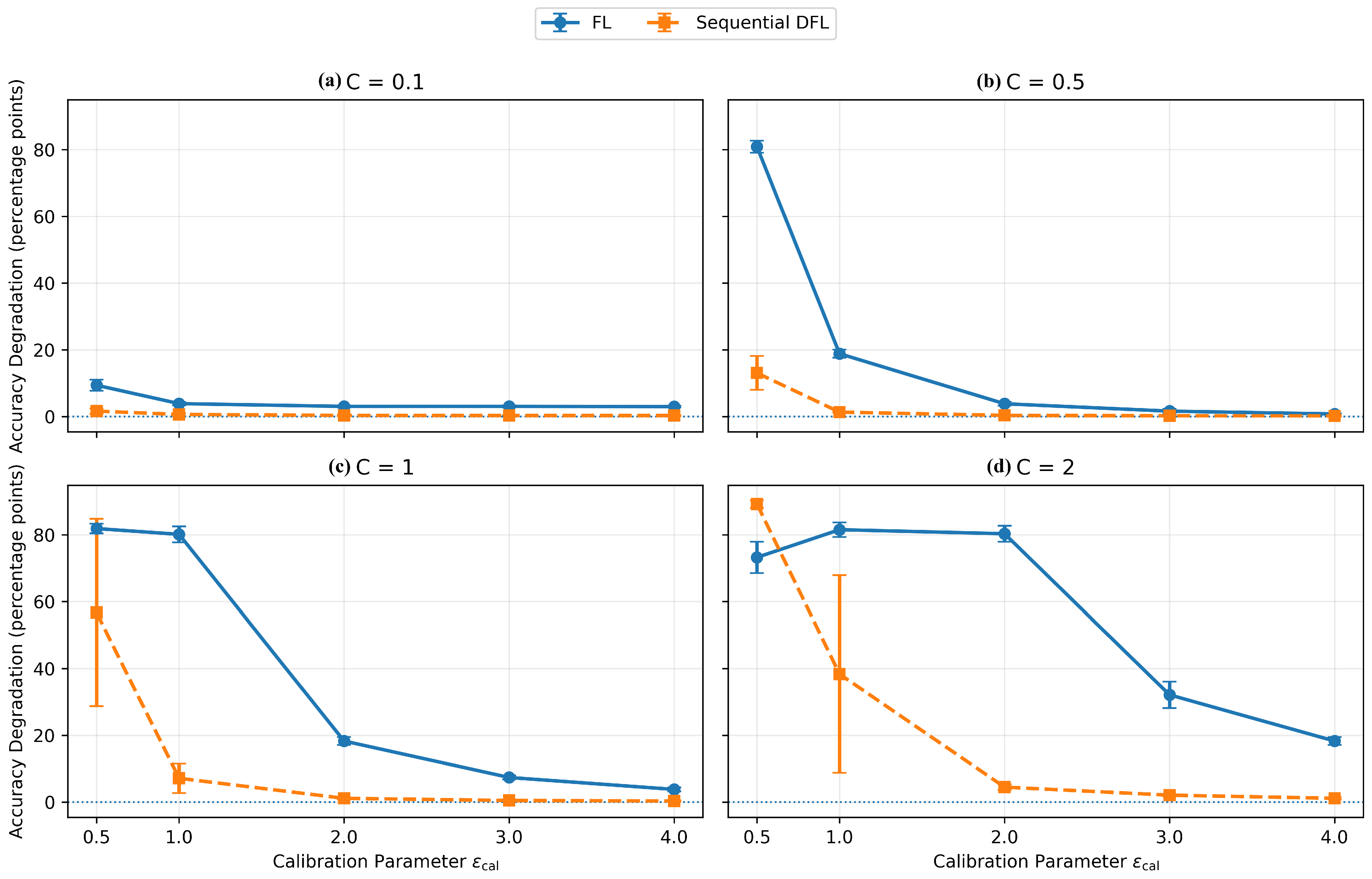
Accuracy degradation was calculated separately for each seed as the difference, in percentage points, between the corresponding No-DP final accuracy and the final accuracy under each matched perturbation setting. The seed-level values were then summarized across the five independent runs. Figure 5 presents the mean accuracy degradation across the four clipping norms, with error bars indicating 95% confidence intervals.

As shown in Figure 5, the magnitude of accuracy degradation differed considerably across the evaluated settings. At $C=0.1$, degradation ranged from approximately 3 to 9 percentage points for FL and from approximately 0.3 to 1.6 percentage points for sequential DFL. At $C=1$ and ${ϵ}_{\mathrm{cal}}=0.5$, the mean degradation was approximately 82 percentage points for FL and 57 percentage points for sequential DFL. Some sequential DFL settings showed wider confidence intervals, indicating greater variation in accuracy degradation across the five independent runs.

To examine the effect of the clipping norm further,

Table 4. Clipping frequency and final test accuracy for both frameworks.

C	${\mathit{ϵ}}_{\mathbf{cal}}$	FL		Sequential DFL
		Clipping (%)	Final Accuracy (%)	Clipping (%)	Final Accuracy (%)
0.1	0.5	$94.59\pm 1.50$ (92.74, 96.45)	$82.75\pm 1.13$ (81.34, 84.15)	$100.00\pm 0.00$ (100.00, 100.00)	$97.26\pm 0.52$ (96.61, 97.91)
	1	$91.03\pm 1.48$ (89.19, 92.86)	$88.27\pm 0.49$ (87.65, 88.88)	$100.00\pm 0.00$ (100.00, 100.00)	$98.26\pm 0.22$ (97.99, 98.53)
	2	$89.10\pm 1.45$ (87.31, 90.90)	$89.10\pm 0.50$ (88.49, 89.72)	$100.00\pm 0.00$ (100.00, 100.00)	$98.55\pm 0.13$ (98.39, 98.71)
	3	$88.72\pm 1.43$ (86.95, 90.50)	$89.10\pm 0.51$ (88.47, 89.73)	$100.00\pm 0.00$ (100.00, 100.00)	$98.59\pm 0.10$ (98.46, 98.72)
	4	$88.56\pm 1.43$ (86.78, 90.35)	$89.16\pm 0.55$ (88.48, 89.84)	$100.00\pm 0.00$ (100.00, 100.00)	$98.59\pm 0.09$ (98.47, 98.71)
0.5	0.5	$25.35\pm 3.02$ (21.60, 29.10)	$11.29\pm 1.49$ (9.44, 13.13)	$100.00\pm 0.00$ (100.00, 100.00)	$85.82\pm 3.98$ (80.87, 90.76)
	1	$6.99\pm 1.21$ (5.48, 8.49)	$73.29\pm 1.09$ (71.94, 74.64)	$100.00\pm 0.00$ (100.00, 100.00)	$97.57\pm 0.17$ (97.36, 97.78)
	2	$0.51\pm 0.19$ (0.27, 0.76)	$88.31\pm 0.54$ (87.64, 88.98)	$9.80\pm 0.45$ (9.24, 10.36)	$98.54\pm 0.24$ (98.24, 98.85)
	3	$0.32\pm 0.17$ (0.11, 0.53)	$90.52\pm 0.68$ (89.68, 91.37)	$9.00\pm 0.00$ (9.00, 9.00)	$98.66\pm 0.21$ (98.40, 98.92)
	4	$0.29\pm 0.16$ (0.09, 0.48)	$91.37\pm 0.46$ (90.80, 91.95)	$8.40\pm 0.55$ (7.72, 9.08)	$98.70\pm 0.22$ (98.43, 98.97)
1.0	0.5	$6.05\pm 1.34$ (4.39, 7.71)	$10.23\pm 1.11$ (8.85, 11.61)	$100.00\pm 0.00$ (100.00, 100.00)	$42.10\pm 22.52$ (14.14, 70.06)
	1	$0.42\pm 0.30$ (0.04, 0.79)	$11.97\pm 1.84$ (9.68, 14.25)	$32.20\pm 12.95$ (16.12, 48.28)	$91.72\pm 3.53$ (87.34, 96.10)
	2	$0.00\pm 0.00$ (0.00, 0.00)	$73.83\pm 1.07$ (72.50, 75.16)	$4.00\pm 0.00$ (4.00, 4.00)	$97.74\pm 0.29$ (97.38, 98.10)
	3	$0.00\pm 0.00$ (0.00, 0.00)	$84.73\pm 0.26$ (84.40, 85.06)	$3.40\pm 0.55$ (2.72, 4.08)	$98.38\pm 0.15$ (98.19, 98.57)
	4	$0.00\pm 0.00$ (0.00, 0.00)	$88.31\pm 0.58$ (87.59, 89.03)	$3.20\pm 0.45$ (2.64, 3.76)	$98.53\pm 0.22$ (98.26, 98.80)
2.0	0.5	$0.72\pm 0.56$ (0.03, 1.42)	$18.87\pm 4.07$ (13.82, 23.92)	$98.60\pm 3.13$ (94.71, 100.00) *	$9.62\pm 0.79$ (8.64, 10.61)
	1	$0.00\pm 0.00$ (0.00, 0.00)	$10.57\pm 1.76$ (8.38, 12.76)	$7.60\pm 0.89$ (6.49, 8.71)	$60.51\pm 23.80$ (30.95, 90.06)
	2	$0.00\pm 0.00$ (0.00, 0.00)	$11.79\pm 1.88$ (9.46, 14.12)	$1.20\pm 0.45$ (0.64, 1.76)	$94.37\pm 0.64$ (93.58, 95.17)
	3	$0.00\pm 0.00$ (0.00, 0.00)	$59.98\pm 3.28$ (55.91, 64.05)	$1.00\pm 0.00$ (1.00, 1.00)	$96.78\pm 0.20$ (96.54, 97.03)
	4	$0.00\pm 0.00$ (0.00, 0.00)	$73.83\pm 1.07$ (72.50, 75.16)	$1.00\pm 0.00$ (1.00, 1.00)	$97.72\pm 0.35$ (97.28, 98.16)

* The upper confidence bound for clipping frequency is limited to 100%. Values are reported as mean ± SD with 95% confidence intervals across five independent runs.

reports the clipping frequency together with the resulting final test accuracy across the evaluated C and ${ϵ}_{\mathrm{cal}}$ settings. Both measures are summarized across the five independent runs using the mean, sample standard deviation, and 95% confidence interval.

As shown in Table 4, clipping frequency generally decreased as C increased, whereas final accuracy varied across the matched perturbation settings. At $C=0.1$, FL clipping remained between $88.56\pm 1.43\%$ and $94.59\pm 1.50\%$, whereas sequential DFL recorded $100\%$ clipping across all five ${ϵ}_{\mathrm{cal}}$ settings. Final accuracy nevertheless remained above $82\%$ for FL and $97\%$ for sequential DFL across these settings. At $C=1$, FL clipping decreased to zero for ${ϵ}_{\mathrm{cal}}\ge 2$, with final accuracy ranging from $73.83\pm 1.07\%$ to $88.31\pm 0.58\%$. For sequential DFL, clipping ranged from $3.20\pm 0.45\%$ to $4.00\pm 0.00\%$ over the same settings, while final accuracy ranged from $97.74\pm 0.29\%$ to $98.53\pm 0.22\%$. At $C=2$ and ${ϵ}_{\mathrm{cal}}=0.5$, the two frameworks showed a different pattern. FL recorded $0.72\pm 0.56\%$ clipping and $18.87\pm 4.07\%$ final accuracy, compared with $98.60\pm 3.13\%$ clipping and $9.62\pm 0.79\%$ final accuracy for sequential DFL.

4.3. Privacy Leakage Analysis

4.3.1. Membership Inference Attack Results

Membership inference was evaluated on the final-round models. The evaluation included the No-DP baseline and the matched-perturbation conditions at $C=1$ and ${ϵ}_{\mathrm{cal}}\in \{0.5,1,2,3,4\}$. Three attack variants were tested separately using confidence, loss, and entropy. Each variant was evaluated using logistic regression (LR) and a multilayer perceptron (MLP). All attacks were evaluated across five independent seeds.

Table 5. Membership inference ROC-AUC results at $C=1$ across five independent seeds.

Setting	Confidence		Loss		Entropy
	LR	MLP	LR	MLP	LR	MLP
FL
No-DP	$0.496\pm 0.004(0.491,0.500)$	$0.502\pm 0.005(0.496,0.509)$	$0.501\pm 0.006(0.495,0.508)$	$0.502\pm 0.005(0.495,0.509)$	$0.497\pm 0.005(0.491,0.503)$	$0.496\pm 0.003(0.492,0.501)$
${ϵ}_{\mathrm{cal}}=0.5$	$0.501\pm 0.003(0.498,0.505)$	$0.498\pm 0.005(0.492,0.504)$	$0.500\pm 0.005(0.494,0.506)$	$0.504\pm 0.003(0.500,0.507)$	$0.501\pm 0.002(0.499,0.503)$	$0.501\pm 0.002(0.498,0.504)$
${ϵ}_{\mathrm{cal}}=1$	$0.502\pm 0.005(0.496,0.508)$	$0.503\pm 0.005(0.496,0.509)$	$0.500\pm 0.003(0.496,0.504)$	$0.502\pm 0.002(0.500,0.504)$	$0.502\pm 0.003(0.498,0.506)$	$0.503\pm 0.003(0.499,0.506)$
${ϵ}_{\mathrm{cal}}=2$	$0.498\pm 0.006(0.491,0.506)$	$0.501\pm 0.002(0.498,0.504)$	$0.505\pm 0.003(0.501,0.508)$	$0.504\pm 0.004(0.499,0.510)$	$0.501\pm 0.007(0.492,0.509)$	$0.497\pm 0.004(0.492,0.502)$
${ϵ}_{\mathrm{cal}}=3$	$0.506\pm 0.004(0.501,0.511)$	$0.505\pm 0.005(0.499,0.512)$	$0.506\pm 0.005(0.500,0.512)$	$0.507\pm 0.004(0.501,0.512)$	$0.507\pm 0.004(0.502,0.511)$	$0.503\pm 0.005(0.497,0.509)$
${ϵ}_{\mathrm{cal}}=4$	$0.505\pm 0.006(0.498,0.512)$	$0.500\pm 0.002(0.497,0.502)$	$0.505\pm 0.005(0.498,0.511)$	$0.501\pm 0.009(0.490,0.512)$	$0.504\pm 0.006(0.497,0.511)$	$0.497\pm 0.004(0.492,0.502)$
Sequential DFL
No-DP	$0.501\pm 0.005(0.495,0.508)$	$0.517\pm 0.005(0.511,0.523)$	$0.502\pm 0.005(0.495,0.508)$	$0.501\pm 0.005(0.495,0.508)$	$0.501\pm 0.006(0.494,0.508)$	$0.517\pm 0.004(0.512,0.522)$
${ϵ}_{\mathrm{cal}}=0.5$	$0.499\pm 0.005(0.493,0.505)$	$0.503\pm 0.003(0.500,0.507)$	$0.499\pm 0.005(0.493,0.506)$	$0.502\pm 0.004(0.497,0.506)$	$0.499\pm 0.005(0.493,0.505)$	$0.501\pm 0.002(0.498,0.503)$
${ϵ}_{\mathrm{cal}}=1$	$0.501\pm 0.008(0.491,0.511)$	$0.504\pm 0.006(0.496,0.512)$	$0.501\pm 0.009(0.490,0.513)$	$0.504\pm 0.008(0.494,0.513)$	$0.496\pm 0.007(0.488,0.504)$	$0.498\pm 0.007(0.490,0.506)$
${ϵ}_{\mathrm{cal}}=2$	$0.501\pm 0.006(0.494,0.508)$	$0.505\pm 0.005(0.499,0.511)$	$0.502\pm 0.005(0.495,0.509)$	$0.506\pm 0.006(0.498,0.513)$	$0.501\pm 0.006(0.494,0.508)$	$0.501\pm 0.005(0.495,0.507)$
${ϵ}_{\mathrm{cal}}=3$	$0.500\pm 0.005(0.494,0.506)$	$0.509\pm 0.007(0.500,0.518)$	$0.500\pm 0.005(0.494,0.506)$	$0.501\pm 0.005(0.495,0.506)$	$0.500\pm 0.005(0.494,0.506)$	$0.509\pm 0.007(0.500,0.517)$
${ϵ}_{\mathrm{cal}}=4$	$0.500\pm 0.005(0.494,0.506)$	$0.507\pm 0.006(0.500,0.514)$	$0.500\pm 0.005(0.494,0.506)$	$0.501\pm 0.004(0.496,0.506)$	$0.500\pm 0.005(0.494,0.506)$	$0.509\pm 0.008(0.499,0.519)$

Abbreviations: FL, federated learning; DFL, decentralized federated learning; LR, logistic regression; MLP, multilayer perceptron. Values are reported as mean ± standard deviation, with the 95% confidence interval shown in parentheses.

reports the ROC-AUC for all attack configurations. The values are reported as mean ± sample standard deviation across the five seeds, together with the 95% confidence interval.

For FL, the mean AUC values across all six attacks were between 0.496 and 0.502 in the No-DP condition. Across the matched-perturbation conditions, the mean values ranged from 0.497 to 0.507. The highest FL mean AUC was $0.507\pm 0.004$ for Loss-MLP at ${ϵ}_{\mathrm{cal}}=3$. Entropy-LR at the same setting also produced a mean AUC of $0.507\pm 0.004$.

For sequential DFL, the No-DP results ranged from 0.501 to 0.517. The highest values were obtained by Confidence-MLP and Entropy-MLP, with mean AUC values of $0.517\pm 0.005$ and $0.517\pm 0.004$, respectively. Their 95% confidence intervals were $(0.511,0.523)$ and $(0.512,0.522)$.

Across the matched-perturbation sequential DFL conditions, mean AUC values ranged from 0.496 to 0.509. At ${ϵ}_{\mathrm{cal}}=0.5$, all six mean AUC values were between 0.499 and 0.503. At ${ϵ}_{\mathrm{cal}}=3$, the Confidence-MLP and Entropy-MLP attacks both reached a mean AUC of 0.509.

4.3.2. Gradient-Leakage Results

Gradient leakage was evaluated at $C=1$ using DLG, iDLG, and InvGrad. The main evaluation was conducted at round 100 and included the No-DP baseline and the matched-perturbation conditions for ${ϵ}_{\mathrm{cal}}\in \{0.5,1,2,3,4\}$. Both FL and sequential DFL were evaluated across five independent seeds.

For each seed, the reconstruction metrics were first averaged across the three evaluated client positions.

Table 6. Gradient-leakage results at $C=1$ across five independent seeds.

Setting	DLG			iDLG			InvGrad
	MSE	PSNR	SSIM	MSE	PSNR	SSIM	MSE	PSNR	SSIM
FL
No-DP	$0.178\pm 0.037$	$7.72\pm 1.07$	$0.033\pm 0.035$	$0.157\pm 0.051$	$8.62\pm 1.68$	$0.060\pm 0.029$	$0.018\pm 0.003$	$17.72\pm 1.02$	$0.383\pm 0.038$
${ϵ}_{\mathrm{cal}}=0.5$	$0.266\pm 0.041$	$5.79\pm 0.65$	$0.005\pm 0.013$	$0.261\pm 0.011$	$5.85\pm 0.20$	$0.003\pm 0.004$	$0.273\pm 0.051$	$5.72\pm 0.80$	$0.007\pm 0.006$
${ϵ}_{\mathrm{cal}}=1$	$0.273\pm 0.012$	$5.65\pm 0.19$	$0.008\pm 0.008$	$0.267\pm 0.012$	$5.74\pm 0.21$	$0.011\pm 0.011$	$0.270\pm 0.028$	$5.74\pm 0.47$	$0.009\pm 0.012$
${ϵ}_{\mathrm{cal}}=2$	$0.257\pm 0.011$	$5.91\pm 0.19$	$0.010\pm 0.010$	$0.250\pm 0.015$	$6.04\pm 0.27$	$0.010\pm 0.006$	$0.234\pm 0.015$	$6.34\pm 0.29$	$0.048\pm 0.012$
${ϵ}_{\mathrm{cal}}=3$	$0.258\pm 0.011$	$5.89\pm 0.19$	$0.007\pm 0.012$	$0.262\pm 0.008$	$5.83\pm 0.14$	$0.005\pm 0.007$	$0.100\pm 0.019$	$10.22\pm 0.78$	$0.180\pm 0.037$
${ϵ}_{\mathrm{cal}}=4$	$0.250\pm 0.019$	$6.10\pm 0.43$	$0.020\pm 0.020$	$0.254\pm 0.019$	$6.03\pm 0.43$	$0.021\pm 0.025$	$0.048\pm 0.013$	$13.71\pm 1.13$	$0.280\pm 0.079$
Sequential DFL
No-DP	$0.256\pm 0.007$	$5.91\pm 0.13$	$0.009\pm 0.007$	$0.252\pm 0.015$	$6.01\pm 0.27$	$0.012\pm 0.011$	$0.036\pm 0.016$	$15.70\pm 1.95$	$0.340\pm 0.038$
${ϵ}_{\mathrm{cal}}=0.5$	$0.273\pm 0.005$	$5.64\pm 0.08$	$0.004\pm 0.006$	$0.272\pm 0.003$	$5.65\pm 0.05$	$0.008\pm 0.004$	$0.261\pm 0.037$	$5.89\pm 0.61$	$0.011\pm 0.012$
${ϵ}_{\mathrm{cal}}=1$	$0.265\pm 0.008$	$5.77\pm 0.12$	$0.004\pm 0.006$	$0.265\pm 0.013$	$5.79\pm 0.22$	$0.008\pm 0.012$	$0.265\pm 0.025$	$5.78\pm 0.43$	$0.019\pm 0.025$
${ϵ}_{\mathrm{cal}}=2$	$0.261\pm 0.004$	$5.85\pm 0.07$	$0.009\pm 0.011$	$0.269\pm 0.013$	$5.71\pm 0.22$	$0.008\pm 0.008$	$0.186\pm 0.043$	$7.44\pm 1.00$	$0.090\pm 0.031$
${ϵ}_{\mathrm{cal}}=3$	$0.265\pm 0.005$	$5.77\pm 0.08$	$0.008\pm 0.004$	$0.271\pm 0.008$	$5.69\pm 0.14$	$0.005\pm 0.013$	$0.143\pm 0.041$	$9.23\pm 1.66$	$0.148\pm 0.048$
${ϵ}_{\mathrm{cal}}=4$	$0.264\pm 0.008$	$5.78\pm 0.14$	$0.004\pm 0.005$	$0.267\pm 0.012$	$5.75\pm 0.21$	$0.006\pm 0.010$	$0.130\pm 0.036$	$10.10\pm 1.69$	$0.184\pm 0.057$

Abbreviations: DLG, Deep Leakage from Gradients; iDLG, Improved Deep Leakage from Gradients; InvGrad, Inverting Gradients; MSE, mean squared error; PSNR, peak signal-to-noise ratio; SSIM, structural similarity index measure. Values are reported as mean ± standard deviation.

reports the resulting mean and sample standard deviation across the five seeds for MSE, PSNR, and SSIM. Lower MSE and higher PSNR and SSIM correspond to greater reconstruction similarity.

For FL, InvGrad produced the highest mean SSIM in the No-DP condition, reaching $0.383\pm 0.038$, compared with $0.033\pm 0.035$ for DLG and $0.060\pm 0.029$ for iDLG. InvGrad also produced the lowest mean MSE of $0.018\pm 0.003$ and the highest mean PSNR of $17.72\pm 1.02$ dB in this condition.

Under the matched-perturbation FL conditions, InvGrad mean SSIM was $0.007\pm 0.006$, $0.009\pm 0.012$, $0.048\pm 0.012$, $0.180\pm 0.037$, and $0.280\pm 0.079$ for ${ϵ}_{\mathrm{cal}}=0.5,1,2,3,$ and 4, respectively. At ${ϵ}_{\mathrm{cal}}=4$, the corresponding mean SSIM values for DLG and iDLG were $0.020\pm 0.020$ and $0.021\pm 0.025$.

For sequential DFL, the highest mean SSIM in the No-DP condition was also observed for InvGrad at $0.340\pm 0.038$, compared with $0.009\pm 0.007$ for DLG and $0.012\pm 0.011$ for iDLG. InvGrad produced a mean MSE of $0.036\pm 0.016$ and a mean PSNR of $15.70\pm 1.95$ dB in this condition.

Across the matched-perturbation DFL conditions, InvGrad mean SSIM was $0.011\pm 0.012$, $0.019\pm 0.025$, $0.090\pm 0.031$, $0.148\pm 0.048$, and $0.184\pm 0.057$ as ${ϵ}_{\mathrm{cal}}$ increased from $0.5$ to 4. At ${ϵ}_{\mathrm{cal}}=4$, DLG and iDLG produced mean SSIM values of $0.004\pm 0.005$ and $0.006\pm 0.010$, respectively.

5. Main Findings and Discussion

The non-IID distribution shown in Figure 3 creates substantial variation in both class composition and sample counts across clients. Table 3 shows different learning behavior between the two frameworks. Within the evaluated experimental configuration, sequential DFL generally reached the target accuracy earlier, stabilized sooner, and achieved higher final accuracy than FL. This difference also appeared under No-DP, indicating that the learning procedure itself influences the observed utility. In FL, local updates are produced independently from the round-start model and then aggregated, whereas sequential DFL updates the model successively as it passes through the participating clients. The sequential procedure therefore produces a different optimization trajectory, which is reflected in the convergence and final-accuracy results.

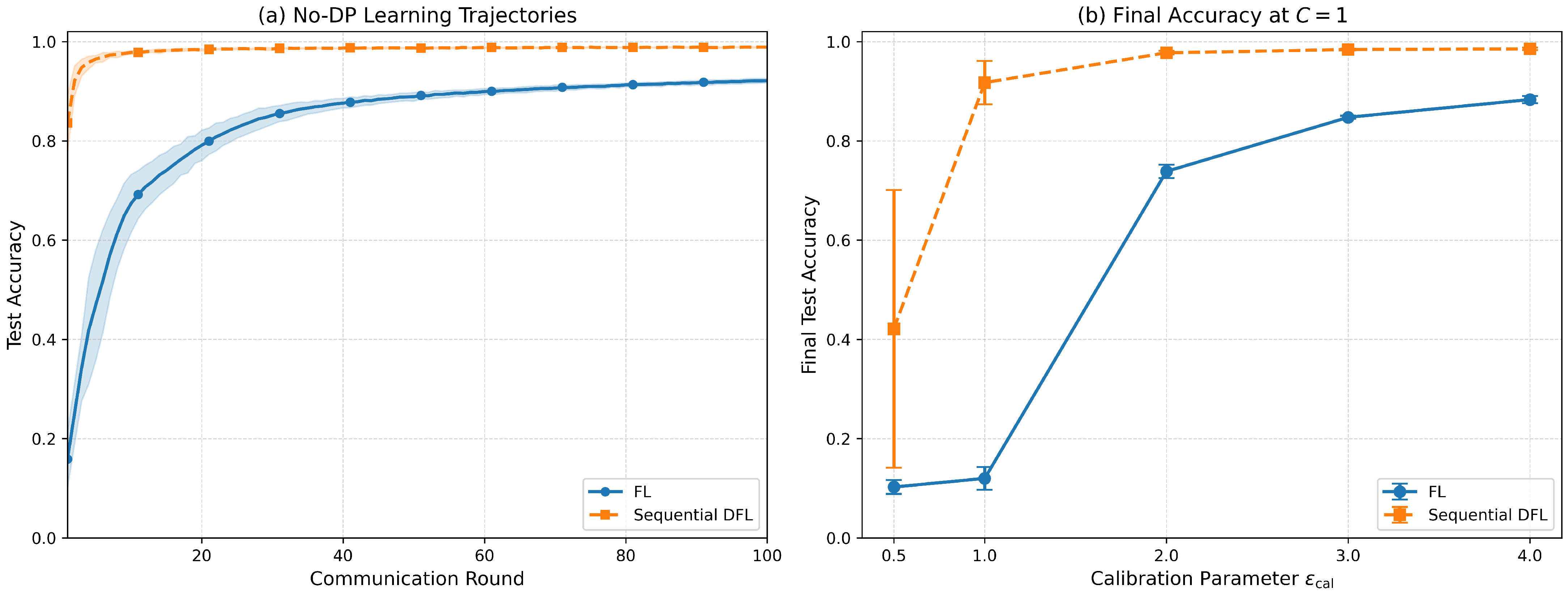
The learning behavior of FL and sequential DFL is further illustrated in Figure 6. Mean test accuracy was calculated across five independent runs. The No-DP learning trajectories were evaluated over 100 communication rounds, whereas final accuracy was compared across the matched-perturbation settings at $C=1$. Shaded regions and error bars represent 95% confidence intervals.

As shown in Figure 6a, sequential DFL reached high No-DP accuracy earlier than FL, whereas FL showed greater variation during the early rounds. Since this difference is present without DP-related perturbation, it reflects differences in the learning procedures. In Figure 6b, sequential DFL maintained higher final accuracy across the evaluated settings, although substantial between-run variation was observed at ${ϵ}_{\mathrm{cal}}=0.5$. The difference between the frameworks became smaller at higher ${ϵ}_{\mathrm{cal}}$ values as both approached their No-DP performance. Overall, the results indicate that utility is influenced by both the learning procedure and its interaction with the perturbation setting.

The broader utility analysis in Figure 4 shows that the response to perturbation also depends strongly on the clipping norm. With the smallest clipping norm, both frameworks retained most of their No-DP utility across the evaluated settings. As C increased, the effect of stronger perturbation became more pronounced, particularly at lower ${ϵ}_{\mathrm{cal}}$. Within the evaluated configurations, sequential DFL retained more utility than FL in many settings, particularly at $C=0.5$ and $C=1$; however, this pattern was not universal. At $C=2$ under the strongest perturbation, FL retained more utility than sequential DFL. The relative utility of the two learning procedures therefore depends on the combination of clipping norm and perturbation setting, rather than on the learning framework alone.

Figure 5 presents the same behavior in terms of loss relative to each framework’s No-DP baseline. Utility degradation remained comparatively small at the lowest clipping norm but became substantial for several combinations of larger C and lower ${ϵ}_{\mathrm{cal}}$. The degradation did not decrease uniformly with increasing ${ϵ}_{\mathrm{cal}}$ across all clipping norms. This further shows that the effect of perturbation cannot be considered independently of the clipping threshold.

The confidence intervals provide additional information about variability across the five independent runs. Although several settings produced relatively narrow intervals, wider intervals were observed for some sequential DFL configurations at lower ${ϵ}_{\mathrm{cal}}$ values. This indicates greater between-run variability in these configurations and shows that the mean alone does not fully describe their learning behavior.

The clipping results in Table 4 help explain this interaction. Frequent clipping did not necessarily correspond to poor utility. At the smallest clipping norm, clipping occurred frequently while both frameworks maintained relatively high accuracy. Conversely, increasing C greatly reduced clipping without consistently improving utility at lower ${ϵ}_{\mathrm{cal}}$ settings. Clipping frequency alone therefore does not explain the observed utility loss.

This behavior follows from the joint role of C in the perturbation mechanism. Increasing C permits larger updates to pass without clipping, but it also increases the absolute Gaussian noise scale for a fixed ${ϵ}_{\mathrm{cal}}$. The utility outcome consequently reflects a balance between update restriction and noise magnitude. This explains why configurations with little or no clipping could still experience substantial accuracy degradation. Taken together, Figure 4 and Figure 5 and Table 4 show that the clipping norm is an important part of the privacy–utility trade-off and that conclusions drawn from a single value of C would not capture the full behavior observed in either framework.

The formal privacy accounting for sequential DFL applies to the perturbed round-end releases. Intermediate models exchanged during token passing are assumed to be protected from adversarial access and are outside the reported privacy guarantee.

The membership-inference results in Table 5 provide a different view of privacy leakage. Despite using confidence-, loss-, and entropy-based attacks with both LR and MLP classifiers, the AUC values remained close to 0.5 in both frameworks. Under the evaluated attack models and final-model access, these values indicate that no substantial membership signal was detected. They do not demonstrate strong membership privacy or exclude leakage under other attacks or access assumptions. One possible explanation is that the relatively simple MNIST classification task provides limited membership information to the evaluated attack models.

The gradient-inversion results in Table 6 reveal a clearer privacy pattern. DLG and iDLG produced little recognizable reconstruction under the matched perturbations, whereas InvGrad recovered substantially more information. InvGrad was therefore the most effective reconstruction method among the three evaluated attacks. Strong perturbation greatly reduced InvGrad reconstruction quality, whereas weaker perturbation allowed progressively more image information to be recovered. Gradient leakage was therefore sensitive to both the perturbation setting and the strength of the reconstruction method.

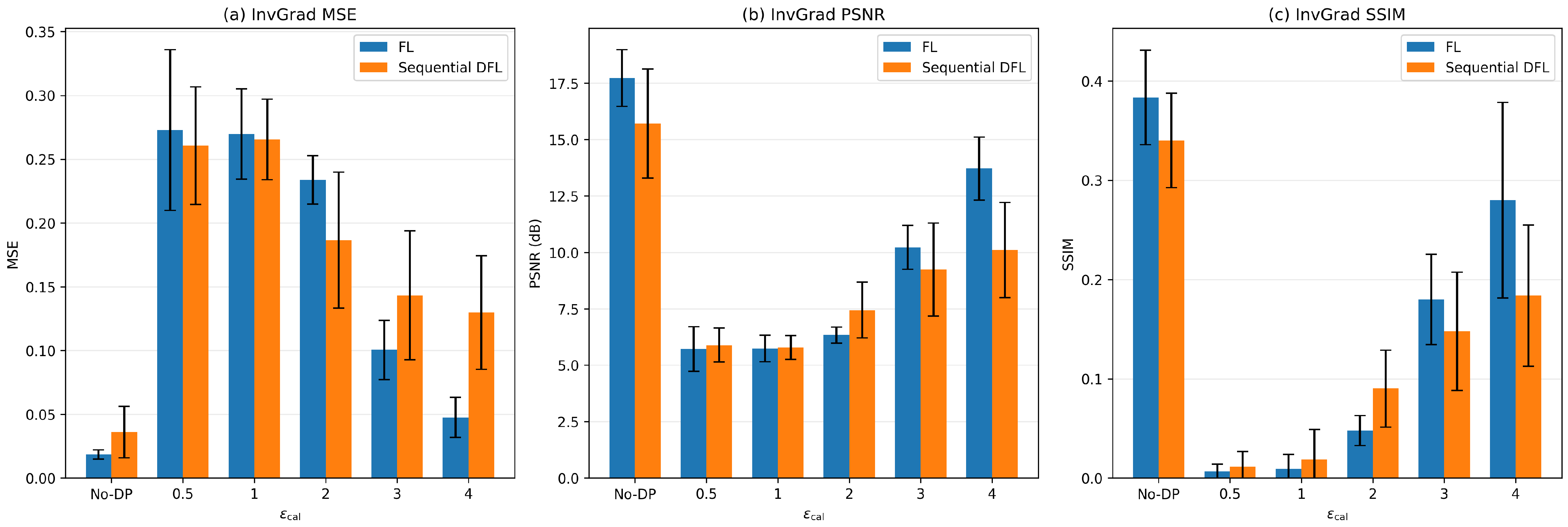
Figure 7 provides a direct comparison of InvGrad reconstruction quality between FL and sequential DFL. Lower MSE indicates better reconstruction quality, whereas higher PSNR and SSIM indicate better reconstruction quality. Better reconstruction quality therefore represents greater information leakage from the observed gradients.

The comparison in Figure 7 shows that neither framework had lower reconstruction leakage under every perturbation setting. FL exposed more reconstructable information under No-DP and at higher ${ϵ}_{\mathrm{cal}}$ settings, whereas sequential DFL showed greater reconstruction quality at ${ϵ}_{\mathrm{cal}}=2$. At the strongest perturbation settings, both frameworks produced low reconstruction quality. The 95% confidence intervals also show noticeable uncertainty in several conditions, particularly for MSE and SSIM, and overlap between the frameworks in some settings. These results suggest greater resistance to InvGrad for sequential DFL in several evaluated conditions, rather than a general privacy advantage of decentralized learning.

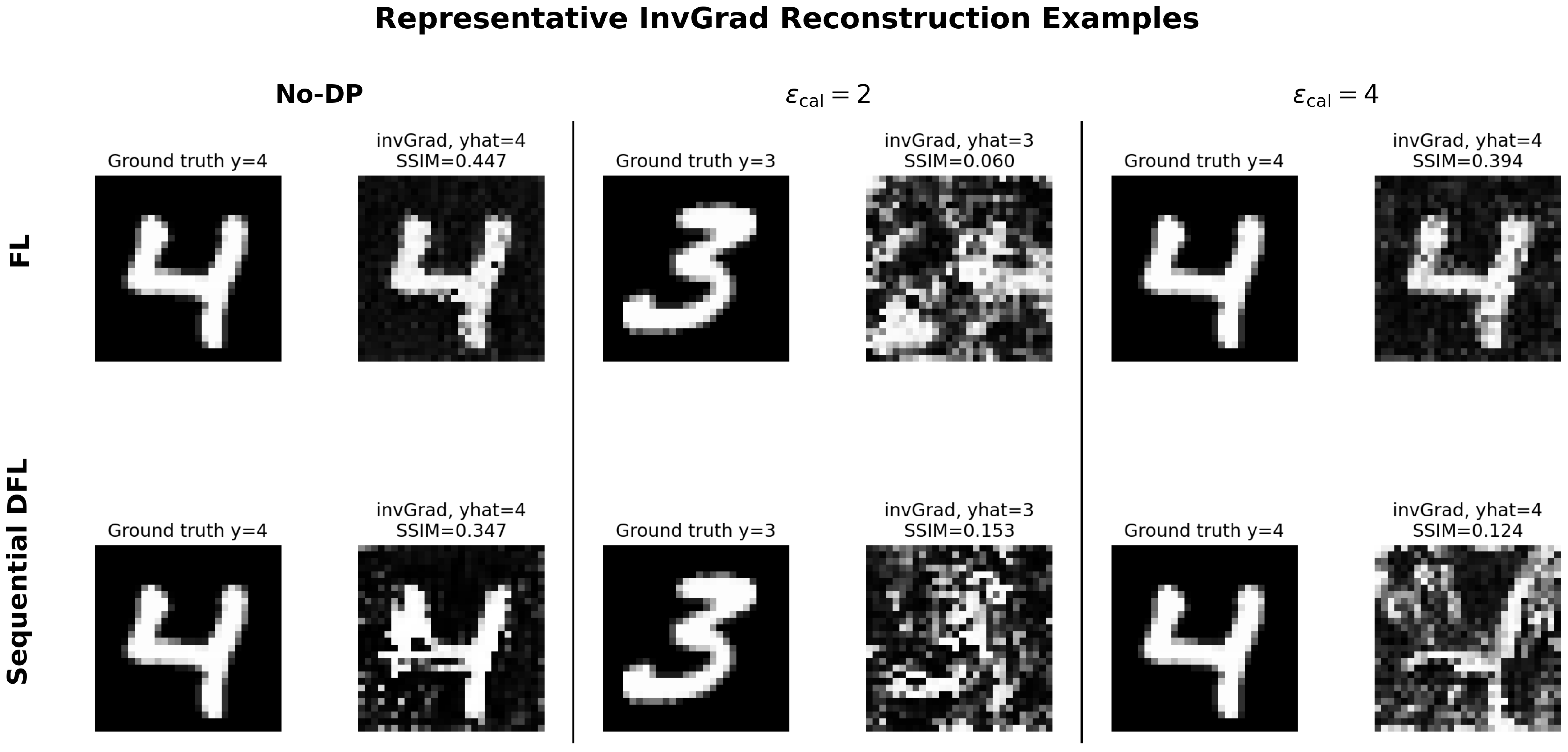
The differences are also visible in the selected InvGrad examples in Figure 8.

As shown in Figure 8, under No-DP, the FL example reveals the original digit more clearly, whereas the sequential DFL reconstruction retains less recognizable structure. At ${ϵ}_{\mathrm{cal}}=2$, the sequential DFL example preserves more image structure than the corresponding FL example, although the reconstructed digit remains visually unclear. At ${ϵ}_{\mathrm{cal}}=4$, recognizable information is again clearer in the FL reconstruction, whereas the sequential DFL example remains more distorted. These examples support the aggregate attack results for the evaluated conditions but do not establish a general difference in privacy between the two frameworks.

Previous research has examined DP extensively in centralized FL, while recent work in decentralized FL has mainly focused on privacy accounting, communication structure, and topology-dependent privacy mechanisms. Direct comparisons between centralized and decentralized learning have also been reported, but these have largely emphasized learning performance, optimization behavior, system characteristics, or specific privacy mechanisms. This study extends the literature by comparing centralized FL and sequential DFL across different DP-related perturbation and clipping settings. It provides empirical evidence of how their interaction influences model utility and privacy leakage in the two evaluated frameworks.

These findings also have practical and research implications. In practice, the clipping norm and perturbation setting should be considered together because both affect the resulting model utility. Privacy evaluation should also consider different attack types because limited leakage under one attack does not necessarily indicate similar resistance to another. From a research perspective, the differences between FL and sequential DFL show that learning and communication structures are important components of privacy-preserving FL. DP-related behavior observed in centralized FL may therefore not directly reflect its behavior in decentralized settings.

The study focuses on one sequential DFL topology, one dataset, and a single model architecture. Accordingly, the conclusions describe the evaluated MNIST dataset, Dirichlet configuration with $\alpha =0.5$, CNN architecture, fixed sequential topology, and attack settings rather than general properties of sequential DFL. The computational cost of the experimental design constrained a broader evaluation, which already combines two learning frameworks, multiple clipping and perturbation settings, five independent seeds, and extensive privacy-leakage evaluations. Further evaluations using additional topologies, datasets, model architectures, data distributions, and adversarial access models are needed to determine the generality of the observed behavior.

6. Conclusions

This study compared centralized FL and sequential DFL to examine how the learning procedure, clipping, and DP-related perturbations affect model utility and privacy leakage. The main goal was to provide a direct empirical comparison of the two frameworks and examine the privacy–utility relationship under different experimental settings. Utility under matched perturbation, formal privacy guarantees, and empirical privacy leakage were evaluated as separate dimensions.

Both frameworks were evaluated using the same MNIST dataset, non-IID data partitioning, CNN architecture, and training configuration. The experiments covered four clipping norms and multiple perturbation settings, together with No-DP baselines. Each experiment was repeated across five independent seeds to account for variation between runs. Learning behavior was evaluated through convergence, stability, final and best accuracy, utility retention, accuracy degradation, and clipping frequency. Formal privacy accounting was used to describe the guarantees associated with the released models. Empirical privacy leakage was evaluated using membership inference and gradient inversion attacks.

Within the evaluated configuration, sequential DFL achieved higher utility and lower gradient-reconstruction quality than FL in several conditions, but these patterns did not hold across all settings. The near-0.5 MIA AUC values indicate that no substantial membership signal was detected under the evaluated attacks; they do not establish strong membership privacy.

The formal privacy guarantee for sequential DFL applies to perturbed round-end releases and assumes that intermediate token-passing models are protected from adversarial access. These conclusions are limited to MNIST, the Dirichlet configuration with $\alpha =0.5$, the evaluated CNN architecture, the fixed sequential topology, and the specified attack settings.

Future work will extend the evaluation to other decentralized communication structures, including gossip-based and random-walk approaches. It will also consider more complex datasets, model architectures, and data distributions.