Article

Joint Modeling of Throughput, Service Time, and Queue Length in IEEE 802.11 WLANs with Frame Aggregation and Unsaturated Traffic Load †

1
School of Computing and Artificial Intelligence (SCAI), Nazarbayev University, Astana 010000, Kazakhstan
2
Department of Electronics Engineering, Hankuk University of Foreign Studies, Yongin-si 17035, Republic of Korea
3
Department of Computer Science and Engineering, Seoul National University, Seoul 08826, Republic of Korea
*
Author to whom correspondence should be addressed.
This paper is an extended version of our paper published in Seytnazarov, S.; Jeong, D.G.; Jeon, W.S. Performance Analysis of IEEE 802.11 WLANs with Frame Aggregation and Unsaturated Traffic Load. In Proceedings of the 2024 IEEE International Black Sea Conference on Communications and Networking (BlackSeaCom), Tbilisi, Georgia, 24–27 June 2024.
Future Internet 2026, 18(9), 451; https://doi.org/10.3390/fi18090451
Submission received: 8 July 2026 / Revised: 12 August 2026 / Accepted: 19 August 2026 / Published: 25 August 2026

Abstract

Frame aggregation is central to modern IEEE 802.11 networks, yet the existing performance models fail to capture how it behaves under usual unsaturated traffic. Some rely on a predefined service-time distribution; others cover only narrow unsaturated cases, such as stations withholding transmission until K packets accumulate or stations being modeled as if they always have a packet queued. This paper develops a performance model for 802.11 networks with frame aggregation under unsaturated traffic in which the aggregation size and service time emerge dynamically from the offered traffic load, the random backoff process, and the number of stations rather than from any of these simplifying assumptions. Beyond throughput, the model derives closed-form estimates of the average aggregation size, service time, and per-station queue length directly from the steady-state distribution of a three-dimensional Markov chain. Performance evaluations across two physical-layer rates (867 and 150 Mbps), two queue capacities, and different numbers of stations show that the proposed model produces throughput and aggregation-size estimates that closely match an event-driven simulator, while the service time and queue-length estimates reflect the model’s own assumption.

1. Introduction

Frame aggregation is an integral part of modern wireless local area networks (WLANs), such as IEEE 802.11n/ac/ax. It can effectively translate the high transmission speed provided by the physical layer (PHY) to high throughput in the medium access control layer (MAC) by sending multiple frames with a single access to the channel [1,2]. More recent amendments target different bottlenecks entirely: IEEE 802.11be introduces multi-link operation to transmit over multiple radio interfaces simultaneously [3], while the forthcoming IEEE 802.11bn coordinates transmissions across access points through spatial reuse [4]; both are outside the scope of the frame-aggregation-focused model developed here.
The literature has many analytical models that analyze the performance of modern WLANs with frame aggregation. Most of them assume that stations always have a saturated traffic load and thus constantly contend for channel access to transmit aggregate frames of maximum/fixed aggregation sizes [5,6,7,8,9]. Some also assume that transmit buffers are always saturated; however, the aggregation size is not fixed but dynamically determined only by the automatic repeat request (ARQ) protocol depending on channel errors [2,10,11,12]. A few other works devised models to evaluate performance with unsaturated traffic loads [13,14,15,16]. However, they assume either a predefined service time distribution [13,14], the stations delay transmission until K packets are accumulated [15], or the stations always have at least one packet to send [16].
The existing modeling approaches do not correctly reflect the operations of WLANs with frame aggregation for the general/unsaturated buffer case for two reasons. First, in practice, WLAN stations usually have unsaturated buffers, so they sometimes do not compete for channel access due to the absence of a packet to send. Second, the aggregation size of the transmission and the duration of the service time are dynamic and vary depending on multiple factors, such as offered traffic load, number of active stations, random backoff process, etc.
In this work, we propose a new performance model for modern WLANs with frame aggregation and unsaturated traffic load. In our model, the stations contend to access the channel only when they have data to send. The aggregation size and service time of each aggregate frame are dynamic and change depending on the current offered load at the station, the random backoff process, the number of contending stations, etc. Beyond throughput, we also derive closed-form estimates of the average aggregation size, MAC service time, and queue length directly from the steady-state distribution of the proposed Markov chain. Performance evaluations with different numbers of stations and various offered traffic loads showed that our model produces network throughput and aggregation-size estimations that closely match the simulation results, while the service time and queue-length estimates remain consistent with the model’s own assumptions.
A preliminary version of this work was presented at the 2024 IEEE International Black Sea Conference on Communications and Networking (BlackSeaCom) [17]. This paper extends that conference version in the following ways. First, we derive two new closed-form performance metrics directly from the steady-state distribution of the proposed Markov chain: the average MAC service time (Section 3.8) and the queue length (Section 3.9), which were not reported in the conference version. Second, we refine the airtime for the successful slots used in the throughput and average-slot-duration equations, replacing the point estimate T s u c c ( N ¯ a g g r ) with the distribution-weighted average T ¯ s u c c (Section 3), which avoids the systematic underestimation of the transmission airtime caused by the convexity of the ceiling operator. Third, we substantially expand the performance evaluation: the conference version validated only throughput for N S T A { 10 , 20 } stations at a single PHY rate (150 Mbps) and a single queue capacity ( Q = 100 ); this paper adds a second PHY rate that is representative of 802.11ac ( R = 867 Mbps), adds N S T A = 30 , and uses two larger queue capacities ( Q = 128 and Q = 256 ). It reports not only throughput but also aggregation size, service time, and queue length across all of these configurations, comparing against two existing analytical models and an event-driven simulator (Section 4 and Appendix A).
The remainder of this paper is organized as follows. In Section 2, we explain the channel access protocol, frame aggregation, and related work. Then, we introduce the proposed model in Section 3. Section 4 discusses the performance evaluations. Finally, Section 5 concludes this paper.

2. Background

2.1. Distributed Coordination Function (DCF) Protocol

The DCF is a channel access protocol used in WLANs. A station that has a data frame to send continuously monitors the channel. If the channel is idle for the duration of the DCF inter-frame space (DIFS), it randomly chooses a new backoff counter from the range [ 0 , W 0 ) , where W 0 is the size of the contention window at backoff stage 0. The sender decrements the counter at the end of every idle standard slot σ and freezes the counter if the channel is detected busy. The frozen backoff counter can be resumed only after an idle DIFS period.
When the backoff counter expires, the sender finally transmits its data frame. If the receiver successfully decodes the data frame, it responds with an acknowledgment frame (ACK) after a period called a short inter-frame space (SIFS).
If the sender receives the ACK within a timeout, it initiates another backoff process if it has any data to send; otherwise, it stays idle while merely monitoring the channel. If the ACK is not received within timeout, the sender enters the next backoff stage to retransmit the failed frame. When the backoff stage is increased, the sender doubles its contention window size, i.e., W i = min ( 2 i · W 0 , W m a x ) , where i [ 0 , r ] . This effectively decreases the chance of a collision. After an idle DIFS period, the sender randomly extracts a new backoff counter from the [ 0 , W 1 ) range and retransmits the frame after the counter expires. However, if the ACK is not received even at the last backoff stage r, the sender discards the data frame and resets its backoff stage to 0.
To avoid the hidden-station problem, the DCF protocol has an optional request-to-send/clear-to-send (RTS/CTS) access mechanism, where the sender transmits an RTS frame when the backoff counter expires. Upon receiving the RTS, the receiver responds with a CTS frame after the SIFS period. If the CTS is received within a timeout, the sender finally transmits the data frame; otherwise, the sender increases the backoff stage and retries the RTS transmission after a new backoff counter expires [1,18,19]. In [20] a simple but more accurate performance model of the legacy DCF protocol without frame aggregation was proposed.

2.2. A-MPDU and BlockAck Frames

In traditional IEEE 802.11 WLAN technologies, such as IEEE 802.11b/a/g, every data frame transmission contained a single packet only. However, starting from the 802.11n standard, the stations can transmit a large data frame called the aggregate MAC protocol data unit (A-MPDU), which includes multiple MPDUs (packets). For example, in an 802.11n WLAN, when the sender’s backoff counter expires, it can transmit up to 64 MPDUs in a single A-MPDU frame. Each MPDU has the sequence number information in its MAC header, and its frame checksum (FCS) field helps the receiver to detect whether the decoded MPDU contains bit errors. To inform the sender about the reception status of the MPDUs, the receiver replies with a block ACK (BlockAck) frame if at least one of the MPDUs is successfully received. It contains a bitmap field that indicates the success/failure status of up to 64 MPDUs. Upon the next channel access, the sender transmits another A-MPDU composed of unsuccessful packets from the previous transmission and new packets (if there are any) [1,2,18,19]. A-MPDU and BlockAck frames are depicted in Figure 1.

2.3. Literature Review

The existing performance models of IEEE 802.11 WLANs with frame aggregation can be categorized into several groups. The models in the first group assume that buffers are always fully saturated and thus stations always contend for channel access to transmit the A-MPDU of the fixed/maximum aggregation size [5,6,7,8,9]. The second group of models also assume saturated buffers and thus all the stations always compete for channel access. However, they consider automatic repeat request (ARQ) protocols [2,10,11,12]. The ARQ protocol controls the aggregation size of each A-MPDU depending on errors in the channel. Therefore, in these models, the aggregation size can always change when the channel is noisy. The models in the first and second groups are good for finding the upper bounds of throughput and delay for saturated buffers. But, in reality, the stations usually have unsaturated buffers, and they compete for channel access only when they have data to send.
The works in the third group model the performance for unsaturated traffic loads. For example, the authors in [13,14] assumed a predefined service time distribution. In another work [15], Kim et al. assumed that the stations defer transmission until K packets are accumulated and new packet arrivals during the backoff period and transmission duration are ignored. There is another work that models a very specific case of unsaturated traffic load, where stations always have at least one packet to send [16]. If the buffer is empty, the model generates a new (dummy) packet to keep it always busy, and therefore the stations constantly contend for channel access. At small offered loads, the probability that buffers are empty is high; therefore, many dummy packets are generated to keep them busy. Thus, the model produces throughput higher than the actual offered load. However, at higher offered loads, the probability that buffers are empty becomes smaller, and thus fewer dummy packets are generated, leading to more accurate throughput estimations. To the best of our knowledge, this model is the most accurate among the existing ones. However, none of the existing frame-aggregation models jointly derive throughput, service time, and queue length from a single model with dynamically sized aggregation. Table 1 summarizes how the proposed model relates to these three groups.
There are several inconsistencies between the existing models and the real operations in WLANs with A-MPDU aggregation. First, in practice, WLAN stations usually have unsaturated buffers, and they only compete for channel access when they have a packet to send. Second, the aggregation size and service time of A-MPDUs change depending on dynamic factors such as offered load, the amount of contending stations, the random backoff timer, etc. Therefore, we can conclude that the existing models do not correctly reflect WLAN operations with A-MPDU aggregation and usual/unsaturated traffic loads.
Frame-aggregation modeling has also been extended to multi-user orthogonal frequency division multiple access (MU-OFDMA) and uplink OFDMA-based random access (UORA) mechanisms introduced in IEEE 802.11ax, under both saturated [21] and nonsaturated [22,23,24] traffic, as well as for downlink scheduling and acknowledgment overhead [25]. However, these works address a fundamentally different channel access mechanism in which an access point coordinates simultaneous transmissions from multiple stations over separate resource units rather than the single-channel DCF/EDCA contention with A-MPDU aggregation studied in this paper.

3. Proposed Performance Analysis Model

In this work, we propose a new performance model of modern WLANs with A-MPDU aggregation and unsaturated loads, where the stations contend for channel access only when they have a packet to send and the aggregation size and service time change depending on the offered traffic load, the number of contending stations, the random backoff process, etc. We make the following assumptions.
1.
Each station is in the communication range of each other;
2.
The transmission channel is ideal, and the decoding errors are caused only by collisions;
3.
Each transmission collides with constant probability (p) regardless of the backoff stage;
4.
The aggregation size of an A-MPDU is maintained during its service.
The first three assumptions are often utilized to simplify the models in the literature [5,6,8,26]. The last one was introduced in our previous work [16,17] and needs more explanation. In practice, the station composes an A-MPDU whenever there is a packet to send (even only one) and starts the backoff process to transmit it, i.e., starts the service of this A-MPDU. The service ends when the BlockAck for this A-MPDU is received or when the station drops this A-MPDU due to an exhausted retry limit. We assume that new packet arrivals during the service of this A-MPDU are accounted for only after the service finishes. Thus, the aggregation size of an A-MPDU is maintained at its initial size; i.e., the A-MPDU cannot include newly arriving packets during its service.
Assumptions 1–3 follow standard practice in this model class [26] and each admits a direct extension. Non-Poisson traffic does not require a different chain: the arrival kernel used in (14) and (15) only needs the arrival-count distribution over a given interval, so replacing the Poisson pmf α j ( t ) with, e.g., a constant-bit-rate or more bursty renewal-process pmf leaves the rest of the model unchanged. Channel decoding errors (Assumption 2) admit a simple extension only in the special case where an error affects the entire A-MPDU, e.g., a deep fade that corrupts the whole PPDU. This can be folded into p by replacing the pure collision probability with a combined failure probability p = 1 ( 1 p ) ( 1 p e ) , where p e is the per-attempt probability that the whole aggregate is lost without altering the chain structure since a wholly lost A-MPDU is already treated identically to a collision. This substitution does not extend to the more common case of a partial error in which only some of the aggregated MPDUs are corrupted: the receiver’s compressed BlockAck bitmap then acknowledges the correctly decoded MPDUs individually, and the station’s next A-MPDU is assembled starting from the first unacknowledged MPDU together with any newly arrived packets, so the resulting aggregation size depends on the location of the error within the aggregate rather than on a single scalar probability. Modeling this partial-error BlockAck-window-driven behavior requires the treatment developed in our earlier work [2] and falls outside the scope of the substitution above. Heterogeneous stations and a backoff-stage-dependent collision probability (Assumption 3) are more structural: they break the symmetry that lets a single tagged-station chain represent every station and would require either a per-class chain coupled through a shared channel state or a stage-dependent p i in place of the constant p in (4)–(9). We leave a full heterogeneous extension to future work but note that the qualitative behavior we validate here—the coupling between queue occupancy and contention—is not specific to the homogeneous case.

3.1. Proposed Three-Dimensional Markov Chain

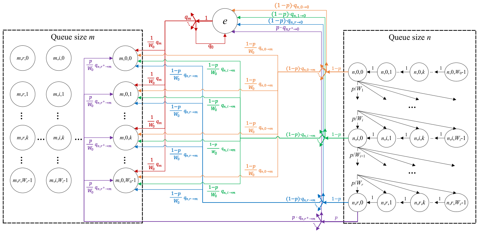
Figure 2 depicts a newly proposed three-dimensional (3D) Markov chain of queue/buffer size, backoff stage, and backoff counter. The model takes a discrete and integer timescale, where the time indices t and t + 1 correspond to the beginnings of two consecutive slots, respectively. The state at t is composed of three components and is represented by { n , i , k } , where
  • n [ 1 , Q ] is the number of packets in the queue/buffer (i.e., the size of the queue/buffer), where Q is the queue capacity in terms of the number of packets;
  • i [ 0 , r ] is the value of the backoff stage, where r is the value of the last backoff stage;
  • k [ 0 , W i ) is the value of the backoff counter, where W i is the size of the contention window at the backoff stage i.
When the station has no packet in its queue, that is, an empty queue, the state is expressed by { e } .
To make the proposed 3D chain more readable, Figure 2 illustrates only the outgoing transitions from queue size n and the incoming transitions to queue size m. Since m and n represent any of the feasible queue sizes in our model, we believe that one can easily illustrate outgoing/incoming transitions from/to any queue size using Figure 2.

3.2. One-Step State Transition Probabilities

Let us derive the state transition probabilities of our Markov chain. We start by exploring the probabilities of transitioning to the state with an empty queue, that is, the state { e } .
P { e | e } = q 0 P { e | n , i , 0 } = ( 1 p ) · q n , i 0 , i [ 0 , r ] P { e | n , r , 0 } = p · q n , r + 0 .
The first equation in (1) corresponds to the probability of staying in the state { e } . q k represents the probability that k packets arrive in an empty queue during an interval of Γ ¯ s l o t , which represents the average slot duration when all other stations except the tagged station contend for channel access and will be derived later. The other two equations are the transition probabilities to the empty state { e } immediately after successful transmission at stage i and unsuccessful transmission at the last stage r, respectively. q n , i k is the probability that the tagged station has k packets in its queue immediately after the A-MPDU is successfully transmitted from the state { n , i , 0 } . q n , r + k is the probability that the station has k packets in its queue immediately after dropping the A-MPDU due to a collision in the state { n , r , 0 } .
P { m , 0 , k | e } = 1 W 0 q m , k [ 0 , W 0 ) P { m , 0 , k | n , i , 0 } = 1 p W 0 q n , i m , k [ 0 , W 0 ) P { m , 0 , k | n , r , 0 } = p W 0 q n , r + m , k [ 0 , W 0 ) .
Equation (2) is for the transition probabilities to the states with stage 0. The first equation expresses the probability of transition after the arrival of m packets in an empty queue during the interval Γ ¯ s l o t . Note that a new backoff counter k is randomly selected from the interval [ 0 , W 0 ) , i.e., with probability 1 W 0 . The remaining equations are probabilities that the station will transition to the state { m , 0 , k } after the successful and unsuccessful service of the current A-MPDU, respectively. The service is unsuccessful if the A-MPDU transmission fails at backoff stage r.
P { n , i , k | n , i , k + 1 } = 1 , i [ 0 , r ] , k [ 0 , W i 2 ] P { n , i , k | n , i 1 , 0 } = p W i , i [ 1 , r ] , k [ 0 , W i ) .
Equation (3) includes the probabilities of one-step transition between the states of the same queue size. The first equation is the probability that the station decrements its nonzero backoff counter at the end of an idle slot. The second equation represents the probability that the transmission from stage i 1 encounters a collision (with probability p), so the station increases its backoff stage and randomly selects a new backoff counter k from the interval [ 0 , W i ) (with probability 1 W i ).
It is important to note that, due to Assumption 4 in the proposed model, there is no transition to the states of other queue sizes upon unsuccessful transmission in stages i [ 0 , r 1 ] .

3.3. Steady-State Probabilities

Let π n , i , k be the steady-state probability of state { n , i , k } . Then, it is easy to obtain the following relationships for n [ 1 , Q ] , i [ 0 , r ] , and k [ 1 , W i ) :
π n , i , k = W i k W i π n , i , 0 π n , i , 0 = π n , 0 , 0 · p i .
Applying (1) to the balance equation of { e } , we get the steady-state probability denoted by π e ,
π e = π e · q 0 + n = 1 Q ( 1 p ) i = 0 r π n , i , 0 · q n , i 0 + p · π n , r , 0 · q n , r + 0 = 1 1 q 0 · n = 1 Q π n , 0 , 0 ( 1 p ) i = 0 r p i · q n , i 0 + p r + 1 · q n , r + 0 .
Using the equations from (2) and the second equation of (4), after some manipulations, we can obtain the steady-state probability of { n , 0 , W 0 1 } as follows:
π n , 0 , W 0 1 = 1 W 0 π e · q n + m = 1 Q π m , 0 , 0 · f ( m , n ) .
where f ( m , n ) : = ( 1 p ) i = 0 r p i · q m , i n + p r + 1 · q m , r + n . Using (6) and the first equation in (4), we obtain the following expression for π n , 0 , 0 :
π n , 0 , 0 = π e · q n + m = 1 Q π m , 0 , 0 · f ( m , n ) = 1 1 f ( n , n ) · π e · q n + m = 1 , m n Q π m , 0 , 0 · f ( m , n ) .
The sum of the steady-state probabilities of all states is equal to 1; that is, π e + n = 1 Q i = 0 r k = 0 W i 1 π n , i , k = 1 . Since π n , i , k = W i k W i · p i · π n , 0 , 0 from (4), we can obtain the following expression:
n = 1 Q π n , 0 , 0 = 2 · ( 1 π e ) i = 0 r p i ( W i + 1 ) .

3.4. Transmission Probability and Throughput

Let τ denote the transmission probability of each station in a given slot. The station transmits whenever its backoff counter expires, that is, only in states { n , i , 0 } . Therefore, τ is given as follows:
τ = n = 1 Q i = 0 r π n , i , 0 = 2 · ( 1 p r + 1 ) · ( 1 π e ) ( 1 p ) i = 0 r p i · ( W i + 1 ) .
According to Assumption 3, each transmission collides with a probability p that can be found using τ as follows [26]:
p = 1 ( 1 τ ) N S T A 1 ,
where N S T A is the total number of stations in the network.
A time slot is idle if none of the stations transmits, contains a successful transmission if only one of the stations transmits, and contains a collision if two or more stations transmit simultaneously. The duration of an idle slot T i d l e simply equals the standard slot time σ and its probability is given as P i d l e = ( 1 τ ) N S T A . The average duration of the success slot, when the request-to-send/clear-to-send (RTS/CTS) access scheme is used, can be calculated as follows:
T s u c c ( l ) = T R T S + T C T S + T P H Y + l · ( L h d r + L p l d ) R · T S Y M · T S Y M + 3 · T S I F S + T B A C K + T D I F S ,
where T R T S , T C T S , T P H Y , T S Y M , T S I F S , T B A C K , and T D I F S represent the durations of the RTS and CTS frames, the PHY preamble and header of the A-MPDU frame, the orthogonal frequency division multiplexing (OFDM) symbol, SIFS, the BlockAck frame, and DIFS, respectively. l is the aggregation size (number of MPDUs) carried by the A-MPDU. L h d r is the total length of the headers of the link, network, and transport layer, while L p l d is the payload length in the transport layer; in all the equations, L h d r and L p l d are expressed in bits, whereas Table 2 lists them in bytes. Finally, R is the PHY transmission rate. The probability of a successful slot is obtained as P s u c c = N S T A · τ · ( 1 τ ) N S T A 1 .
Because the ceiling operator in (11) is applied per transmission, the network-wide average successful-slot duration is not T s u c c ( N ¯ a g g r ) , i.e., T s u c c ( · ) evaluated at the average aggregation size N ¯ a g g r from (18). Instead, it is the distribution-weighted average over all queue sizes,
T ¯ s u c c = n = 1 Q π n , 0 , 0 · T s u c c ( l n ) n = 1 Q π n , 0 , 0 ,
where l n = min ( A , n ) is the aggregation size for the queue size n. Since the ceiling function is convex, T ¯ s u c c T s u c c ( N ¯ a g g r ) ; using the latter in place of (12) underestimates the average transmission airtime and consequently inflates the estimated throughput. We therefore use T ¯ s u c c instead of T s u c c in (13) and (16).
The duration of a collision slot with RTS/CTS is much shorter than the duration of a success slot and can be found by T c o l l = T R T S + T S I F S + T C T S + T D I F S , and its probability is given by P c o l l = 1 P i d l e P s u c c . The system throughput is defined as the average payload length successfully transmitted over the average slot time.
S = P s u c c · N ¯ a g g r · L p l d P i d l e · σ + P s u c c · T ¯ s u c c + P c o l l · T c o l l .

3.5. Offered Load and Service Time Relationship

Let Λ be the total traffic load offered by the network in bits per second (bps). Then, each station has a packet arrival rate of λ = Λ / ( N S T A · L p l d ) packets per second. Assuming Poisson packet arrivals (i.e., exponentially distributed packet inter-arrival times), let us denote by α j ( t ) the probability that j packets arrive during a time interval of length t, and then α j ( t ) = ( λ · t ) j · e λ · t / j ! .
Recall that Γ ¯ s l o t is the average duration of the slot when all other stations except the tagged station compete for channel access. Since the station that has no packet does not contend for channel access, Γ ¯ s l o t can be referred to as the average slot duration of the station in an empty state. We can obtain q m , which is the probability that m packets arrive in the empty queue during the time interval Γ ¯ s l o t as follows:
q m = α m ( Γ ¯ s l o t ) , m [ 0 , Q ) 1 j = 0 Q 1 q j , m = Q .
The probability of having m packets in the queue right after a successful transmission from state { n , i , 0 } is given by
q n , i m = α m ( T n , i ) , n [ 1 , A ] , m [ 0 , Q ) α m n + A ( T n , i ) , n ( A , Q ] , m [ n A , Q ) 1 j = 0 Q 1 q n , i j , n [ 1 , Q ] , m = Q 0 , otherwise ,
where i [ 0 , r ] , T n , i is the average service time of the A-MPDU that was successfully transmitted from state { n , i , 0 } , and A is the maximum aggregation size.
q n , r + m , the probability of having m packets right after an A-MPDU is dropped due to unsuccessful transmission from state { n , r , 0 } , is also obtained from (15) by replacing T n , i with T n , r + , where T n , r + is the average time to drop an A-MPDU for a queue size of n.
To calculate q m , q n , i m , and q n , r + m , we should know Γ ¯ s l o t , T n , i , and T n , r + for all n and i. In [27], Raptis et al. proposed to derive Γ ¯ s l o t as follows. Let us denote by β i d l e the probability that none of the remaining N S T A 1 stations transmits in a random slot; then β i d l e = ( 1 τ ) N S T A 1 . In addition, the probability that only one station among N S T A 1 stations transmits is β s u c c = ( N S T A 1 ) · τ · ( 1 τ ) N S T A 2 . And, let β c o l l = 1 β i d l e β s u c c . Then
Γ ¯ s l o t = β i d l e · σ + β s u c c · T ¯ s u c c + β c o l l · T c o l l .
Next, we calculate T n , i , the average (successful) service time of the A-MPDU that is successfully transmitted at the i-th stage of queue size n,
T n , i = Γ ¯ s l o t j = 0 i W j 1 2 + i · T c o l l + T s u c c , n ,
where i [ 0 , r ] , and T s u c c , n is the duration of a successful slot that contains a successful A-MPDU transmission from the states with a queue size of n. T s u c c , n = T s u c c ( l n ) is obtained from (11) with l = l n = min ( A , n ) , the aggregation size for queue size n. The first and second terms in (17) are the average time spent decrementing the backoff counters and the total time spent on collisions, respectively. The average time to drop the A-MPDU due to an exhausted retry limit can be calculated as T n , r + = Γ ¯ s l o t · j = 0 r W j 1 2 + ( r + 1 ) · T c o l l .

3.6. Average Aggregation Size

The average aggregation size can be obtained using steady-state probabilities. After some manipulations, we will have
N ¯ a g g r = i = 0 r p i · ( W i + 1 ) 2 · ( 1 π e ) n = 1 Q ( l n · π n , 0 , 0 ) .
In (18), since packets are aggregated only when the queue is not empty, the term is divided by ( 1 π e ) for normalization purposes; equivalently, N ¯ a g g r is the π n , 0 , 0 -weighted mean of the per-state aggregate l n = min ( A , n ) , normalized by n = 1 Q π n , 0 , 0 rather than by 1 π e directly, the two being related through the closure in (8). Now, we can numerically solve the system of equations that includes the global balance equation and the equations to find N ¯ a g g r , τ , p, π e , and π n , 0 , 0 for n [ 1 , Q ] .

3.7. Numerical Solution Procedure

Although the system in (1)–(18) appears to couple p, τ , π e , π n , 0 , 0 , and N ¯ a g g r through several nonlinear relations, it reduces to a single scalar fixed point. For a fixed collision probability p, the queue-state distribution { π n , 0 , 0 } n = 1 Q together with π e is the unique stationary solution of an ( Q + 1 ) -dimensional linear system consisting of the Q balance Equation (7) and the normalization (8) given the average slot duration Γ ¯ s l o t ; this linear system is solved exactly (no iteration) for a candidate Γ ¯ s l o t , and Γ ¯ s l o t itself is then updated from the resulting N ¯ a g g r and τ via (16) and iterated to convergence, which we term the inner fixed point. The remaining nonlinearity is the single scalar coupling p τ Γ ¯ s l o t N ¯ a g g r τ , so the full system is solved by finding the root of (10), written as
F ( p ) : = p 1 ( 1 τ ( p ) ) N S T A 1 = 0 ,
where τ ( p ) is obtained from the converged inner fixed point at that p using a bracketed root-finding method (Brent’s method) on p ( 0 , 1 ) . Because τ ( p ) is monotonically increasing in p and 1 ( 1 τ ( p ) ) N S T A 1 is monotonically increasing in τ , F is monotone, so the root is unique for every offered load: the solution does not depend on the initial guess, and there is no spurious high-load or low-load branch. Per outer evaluation, the dominant cost is the linear solve for { π n , 0 , 0 } , which is O ( Q 3 ) in general (or O ( Q 2 ) exploiting the transition matrix’s banded structure from the bounded arrival window); the inner fixed point on Γ ¯ s l o t and the outer root search each converge in a small load-independent number of iterations in practice. We use a convergence tolerance of 10 10 on both fixed points.

3.8. Average Service Time

We define the average MAC service time D ¯ as the mean time from the instant an A-MPDU starts its service (i.e., becomes the head-of-line frame and enters the backoff stage 0) until it is successfully transmitted, averaged only over successful transmissions (dropped A-MPDUs are excluded). MAC service time is also often referred to as access delay. From the first equation in (4), π n , i , 0 = π n , 0 , 0 · p i , and every state { n , i , 0 } succeeds with the same probability ( 1 p ) regardless of n and i; hence ( 1 p ) cancels in the conditional average, and D ¯ can be expressed directly in terms of the service time T n , i from (17):
D ¯ = n = 1 Q i = 0 r π n , 0 , 0 · p i · T n , i n = 1 Q i = 0 r π n , 0 , 0 · p i .
Equation (20) accounts for the time spent decrementing the backoff counter, including slots frozen by other stations’ transmissions and embedded in Γ ¯ s l o t , the collisions experienced before the eventual success, and the final successful transmission itself.

3.9. Average Queue Length

The average number of packets n ¯ in a station’s queue is the expectation of the queue size n over the steady-state distribution of the chain. A queue of size n is distributed across all backoff stages i and counters k, so its marginal probability is i = 0 r k = 0 W i 1 π n , i , k , and the average queue length is
n ¯ = n = 1 Q n i = 0 r k = 0 W i 1 π n , i , k n = 1 Q i = 0 r k = 0 W i 1 π n , i , k = n = 1 Q n · π n , 0 , 0 n = 1 Q π n , 0 , 0 .
The first expression sums over the full steady-state distribution, excluding the empty state { e } ; the second equality follows from (4) since the stage-and-counter sum i = 0 r p i ( W i + 1 ) / 2 is independent of n and therefore cancels between the numerator and denominator. Because every state contributes with equal weight, n ¯ equals the queue occupancy sampled at the instants an A-MPDU is formed: each service passes through exactly one state { n , 0 , 0 } , at which the queue holds n packets before the aggregate of size l n = min ( A , n ) is drawn, so π n , 0 , 0 weights each formation once. It is thus an event average over formation instants rather than a holding-time-weighted time average.
Because both (20) and (21) inherit Assumption 4, the aggregation size of an in-service A-MPDU is frozen at l n = min ( A , n ) , and packets that arrive during its service are accounted for only afterward; they represent the service time and the formation-instant queue length of the idealized model rather than of a system that continuously tops up an in-flight A-MPDU during backoff. Because the queue is sampled at the instants an A-MPDU is formed, n ¯ in (21) corresponds directly to the backlog an event-driven simulator observes when it assembles each A-MPDU. Section 4 shows that this assumption has a negligible effect on the accuracy of throughput and aggregation size and that the formation-instant queue length tracks the simulator closely at light-to-moderate load, with the model’s service time and queue length departing from the simulator only as the offered load approaches saturation.

4. Performance Evaluations

4.1. Evaluation Settings

To validate the proposed model, we compare it against two existing analytical models and an event-driven IEEE 802.11n/ac simulator [28] run in two modes. The first analytical baseline, labeled Existing 3D, is the three-dimensional model of [16], which we previously identified as the most accurate existing model, although one that assumes that stations always have at least one packet to send. The second, labeled Existing 2D, is the aggregation model of [15], which is built on a two-dimensional backoff chain and transmits a fixed maximum-size aggregate; it therefore does not capture how the batch size varies with the offered load. For the simulator, the default mode (labeled simulator) lets an A-MPDU keep aggregating packets that arrive during its backoff, whereas the second mode (labeled simulator (A4)) freezes the A-MPDU at the instant its service starts, thereby enforcing Assumption 4. The default simulator thus differs from the proposed model only in Assumption 4, while simulator (A4) shares all of the proposed model’s assumptions, so the two simulator curves bracket the effect of Assumption 4 on the service time and queue length.
We ran the comparison for two PHY rates representative of 802.11ac ( R = 867 Mbps) and 802.11n ( R = 150 Mbps), two queue capacities ( Q = 128 and Q = 256 packets), N S T A { 10 , 20 , 30 } stations, and offered loads Λ swept from 50 to 3000 Mbps at R = 867 Mbps and from 20 to 600 Mbps at R = 150 Mbps. The main text presents the R = 867 Mbps results; the corresponding R = 150 Mbps results, obtained with the identical methodology, are reported in Appendix A. Each simulator data point is the average of five independent replications with different random seeds; each replication simulates 50 s of channel activity, of which the first 1 s is discarded as a warm-up transient so that only steady-state samples contribute to the reported averages. The results are highly repeatable across seeds: the half-width of the 95 % confidence interval (Student’s t, four degrees of freedom) stays below 1.5 % of the mean for the throughput and aggregation size, below 1.7 % for the service time, and below 3.4 % for the queue length over the entire load range for both simulator variants. Because these intervals are smaller than the plot markers, we omit error bars from the figures for readability. Table 2 summarizes the resulting parameter set.

4.2. Network Throughput

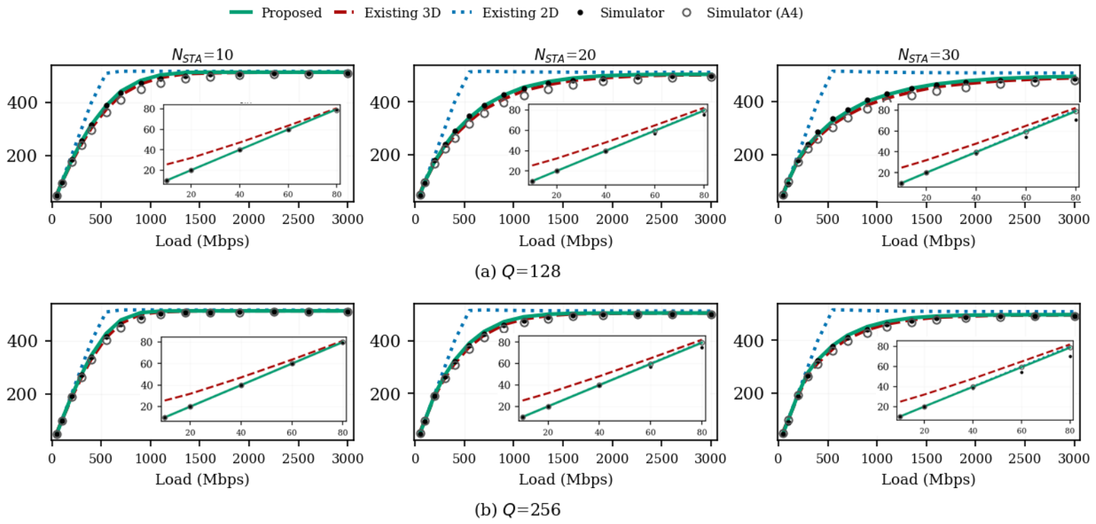
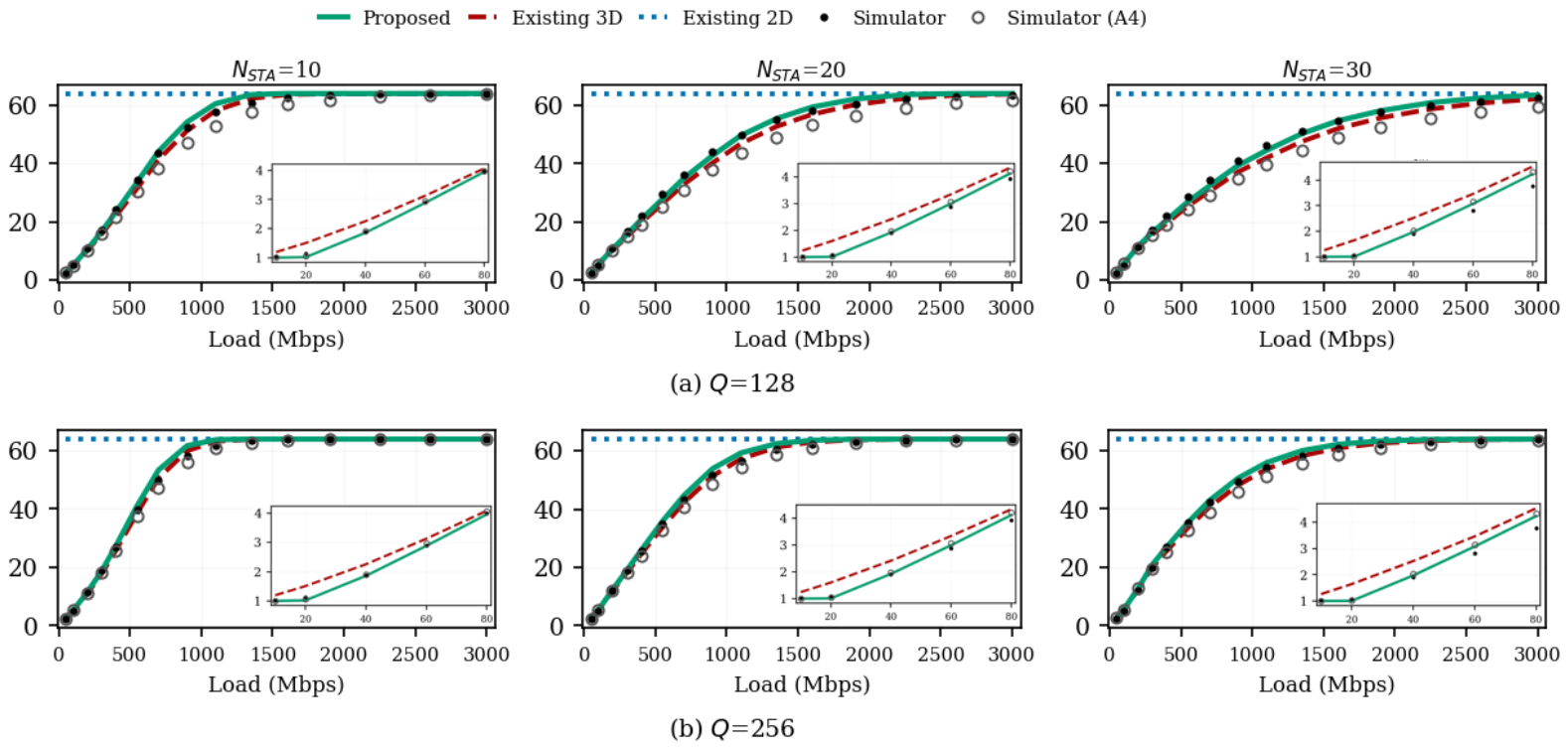
Figure 3 shows the average network throughput against the offered load, with one panel per ( N S T A , Q ) configuration. At light load, the proposed model and both simulator variants track the offered load almost exactly since collisions are rare. As load increases, growing contention slows the rate of throughput increase until it saturates. The proposed model closely tracks the simulator across the full range of loads, station counts, and queue capacities, correctly reproducing both the linear region and the saturation point, with only minor deviations attributable to Assumption 4 and anomalous slot effects [29]. The saturation level is sensitive to N S T A : at Q = 128 it falls from about 513 Mbps at N S T A = 10 to about 504 Mbps at N S T A = 20 and about 495 Mbps at N S T A = 30 , while increasing Q from 128 to 256 changes it by less than 1 % . This N S T A dependence arises because the collision duration T c o l l is rate-independent while the successful-transmission airtime is short at this high rate, so collisions consume a relatively larger share of the channel time. The same measurements at R = 150 Mbps (Appendix A) confirm this interpretation: there the saturation throughput spans only about 1 % across the same three station counts ( 126.3 , 125.8 , and 124.8 Mbps), roughly a third of the spread observed at R = 867 Mbps because the longer data airtime at the lower rate dilutes the fixed collision cost. Existing 3D matches the proposed model and the simulator near saturation but overestimates throughput at light load, where it assumes a non-empty buffer; this light-load gap is shown in detail in the inset panels of Figure 3. Existing 2D overestimates throughput over a much wider range. For example, at N S T A = 30 and Q = 128 , it reports about 400 Mbps at Λ = 400 Mbps, where the proposed model and simulator deliver only about 275–285 Mbps. This is because it always transmits a full A = 64 aggregate regardless of the actual backlog. All the curves converge as the network approaches saturation and buffers are rarely empty.
Regarding the two remaining parameters, increasing N S T A both lowers the saturation throughput (as noted above) and makes the network reach saturation at a lower per-station offered load since the aggregate collision probability at a given total load grows with the number of contending stations. Increasing Q from 128 to 256 packets has almost no effect on throughput: once a station has a packet to send, additional buffer space beyond the aggregation limit A = 64 does not change how efficiently the channel is used, so a larger queue capacity mainly postpones packet loss rather than increasing throughput.

4.3. Aggregation Size

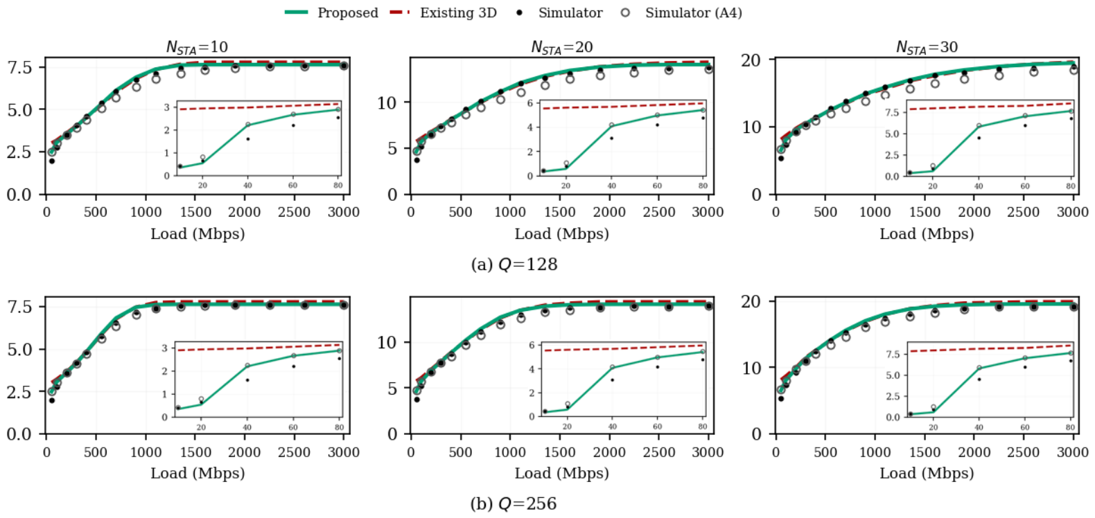
Figure 4 shows the average aggregation size N ¯ a g g r . The proposed model and both simulator variants agree closely at all loads, station counts, and queue capacities, confirming that the distribution-weighted airtime correction in (12) reproduces the batching behavior observed in the simulator; Existing 3D agrees as well except at light load, where it slightly overestimates the aggregate due to its non-empty-buffer assumption, as shown in the inset panels of Figure 4. Existing 2D, by construction, reports a constant N ¯ a g g r = A = 64 at every load and therefore departs sharply from the others at light-to-moderate load, where the true aggregate is far smaller; this is the direct cause of its throughput overestimate noted above. The larger queue capacity ( Q = 256 ) increases the saturation aggregation size only modestly relative to Q = 128 since a station’s backlog can grow further before hitting the buffer cap but A = 64 already bounds the maximum batch size. Increasing N S T A lowers the aggregation size at a given offered load since more stations sharing Λ means each sees a lower arrival rate and fills its buffer more slowly; at this high rate, however, the saturation aggregation size approaches the cap A = 64 for all three station counts (e.g., at Q = 128 and Λ = 3000 Mbps it is 64.0 , 64.0 , and 63.5 MPDUs for N S T A = 10 , 20, and 30, respectively).

4.4. MAC Service Time

Figure 5 shows the average MAC service time D ¯ against offered load. The service time is highly sensitive to N S T A : at a given load, more contending stations mean more frequent collisions and longer backoff freezes, so each A-MPDU needs more attempts and more waiting time before a successful transmission, and D ¯ grows accordingly (e.g., near saturation at Q = 128 it rises from about 7.6 ms at N S T A = 10 to about 14.1 ms at N S T A = 20 and about 19.5 ms at N S T A = 30 ). The service time also scales inversely with the PHY rate: the corresponding values at R = 150 Mbps are about 31.0 , 56.5 , and 75.0 ms (Appendix A), roughly four times larger since each A-MPDU occupies the channel proportionally longer. Increasing Q also increases the estimated delay near saturation because a larger buffer keeps more packets queued rather than dropping them, and the extra packets each contribute additional waiting time as the station repeatedly contends to clear the backlog; consequently, Q = 256 shows a modestly higher service time than Q = 128 at heavy load for the same N S T A .
Comparing the proposed model to the default simulator, the service time shows a small but persistent gap at both queue capacities: the proposed model runs slightly above the simulator, most visibly at moderate-to-high load. This gap is a structural consequence of Assumption 4 rather than a modeling error: because the proposed model freezes the aggregation size of an A-MPDU at the instant it starts service, it forms slightly smaller batches than the default simulator (which keeps topping up the in-flight A-MPDU with new arrivals during backoff), so it needs marginally more transmissions to clear the same offered load even though the resulting throughput is nearly unaffected. Simulator (A4), which enforces the same frozen-aggregate assumption, lies closest to the proposed model and confirms this interpretation, while Existing 3D matches the proposed model except at light load, where it overestimates the service time, as shown in the inset panels of Figure 5.

4.5. Per-Station Queue Length

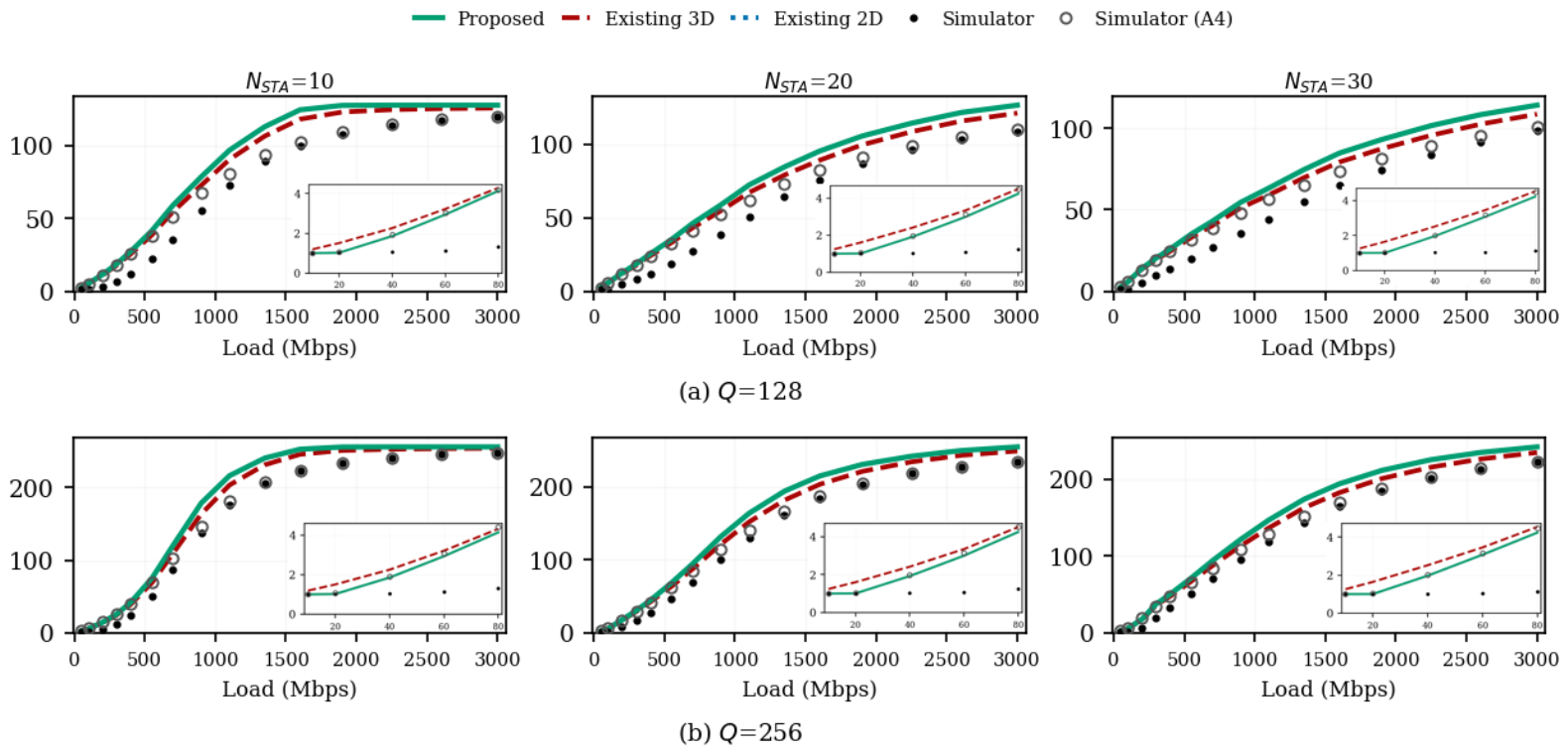
Figure 6 shows the average per-station queue length n ¯ , sampled at the A-MPDU formation instants as defined in (21). The average queue length is, unsurprisingly, most sensitive to Q: a larger buffer allows more packets to accumulate before being dropped, so n ¯ under Q = 256 visibly exceeds Q = 128 once the network approaches saturation, while the two curves are nearly indistinguishable at light load, where the buffer rarely fills regardless of its capacity. The effect of N S T A is more subtle: since Λ is the total load offered on the network, more stations imply a lower arrival rate per station, so, for the same Λ and Q, the queue length per station near saturation tends to be lower for larger N S T A (e.g., at Q = 128 and Λ = 3000 Mbps, the proposed model’s n ¯ falls from about 128 packets at N S T A = 10 to about 127 packets at N S T A = 20 and about 114 packets at N S T A = 30 ), although each station’s individual service time is longer.
Comparing the proposed model to the two simulator variants, the formation queue length agrees closely at light-to-moderate load—a direct benefit of sampling the backlog at the A-MPDU formation instants, exactly as the simulator does—and increasingly overshoots as the network approaches saturation, where the proposed model lies above both the default simulator and simulator (A4) (for example, at N S T A = 30 and Q = 128 , it predicts about 114 packets against 99 and 101 for the two simulators). The two simulator curves remain close to each other, with simulator (A4) marginally higher, indicating that, near saturation, the residual gap is only partly attributable to Assumption 4. Existing 3D tracks the proposed model closely except at light load, where the same non-empty-buffer assumption causes it to overestimate the queue length, as shown in the inset panels of Figure 6.

5. Conclusions

We proposed a new performance model for modern IEEE 802.11 WLANs with A-MPDU aggregation and unsaturated traffic loads. The model is based on a 3D Markov chain where the aggregation size and service time of each A-MPDU are dynamically determined by several factors, such as the current offered traffic load, the number of competing stations, the random backoff process, etc. Beyond throughput, we derived closed-form expressions for the average aggregation size, the average MAC service time, and the average per-station queue length directly from the steady-state distribution of the proposed chain. Across two PHY rates (867 and 150 Mbps), two queue capacities ( Q = 128 and Q = 256 ), and N S T A { 10 , 20 , 30 } stations, the proposed model produces throughput and aggregation-size results that closely match an event-driven simulator over the full range of offered traffic loads. The service-time and queue-length estimates track the simulator less tightly, with a load-dependent gap that we attribute to Assumption 4—the aggregation size of an A-MPDU is frozen for the duration of its service—rather than to an error in the chain itself. Relaxing this assumption by feeding arrivals during backoff back into the aggregation-size distribution is a natural direction for future work to close the remaining service-time and queue-length gap without affecting the already accurate throughput and aggregation-size predictions.

Author Contributions

Conceptualization, S.S. (Shinnazar Seytnazarov); methodology, S.S. (Shinnazar Seytnazarov), D.G.J. and W.S.J.; software, S.S. (Shinnazar Seytnazarov); validation, S.S. (Shinnazar Seytnazarov), S.S. (Sain Saginbekov), D.G.J. and W.S.J.; formal analysis, S.S. (Shinnazar Seytnazarov); investigation, S.S. (Shinnazar Seytnazarov); resources, S.S. (Shinnazar Seytnazarov); data curation, S.S. (Shinnazar Seytnazarov); writing—original draft preparation, S.S. (Shinnazar Seytnazarov); writing—review and editing, S.S. (Shinnazar Seytnazarov), S.S. (Sain Saginbekov), D.G.J. and W.S.J.; visualization, S.S. (Shinnazar Seytnazarov). All authors have read and agreed to the published version of the manuscript.

Funding

This research was funded by the Nazarbayev University Social Policy Grant (201705 SPG).

Institutional Review Board Statement

Not applicable.

Informed Consent Statement

Not applicable.

Data Availability Statement

The data presented in this study are available on request from the corresponding author.

Conflicts of Interest

The authors declare no conflicts of interest.

Appendix A. [Results at R = 150 Mbps]
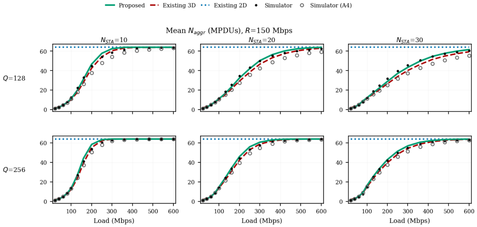
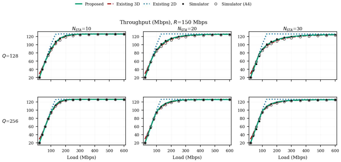
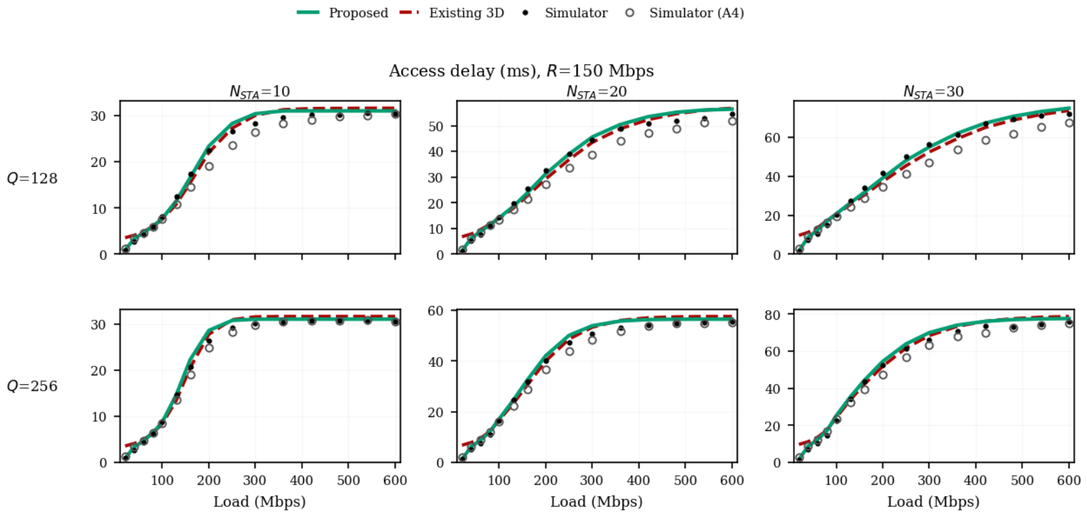
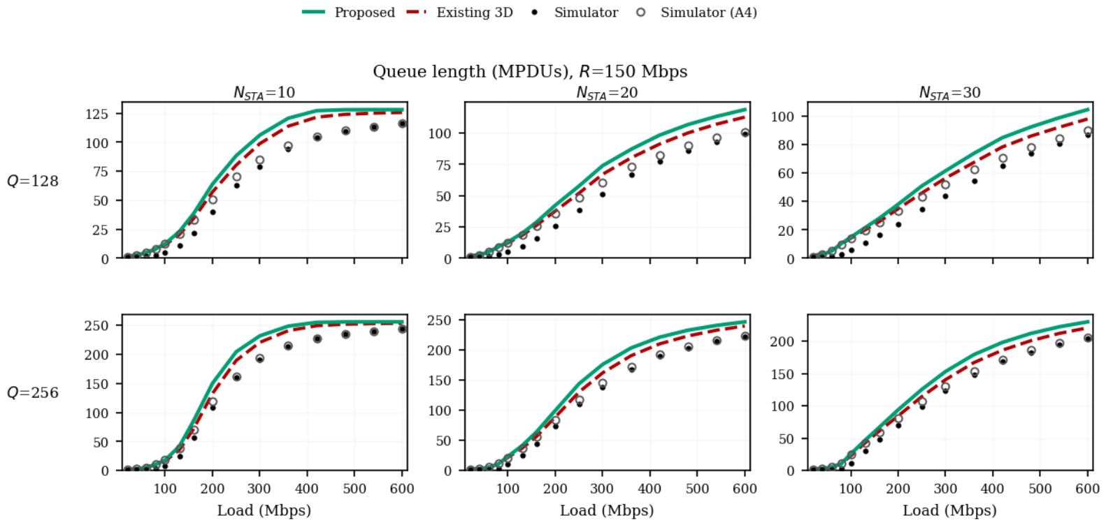
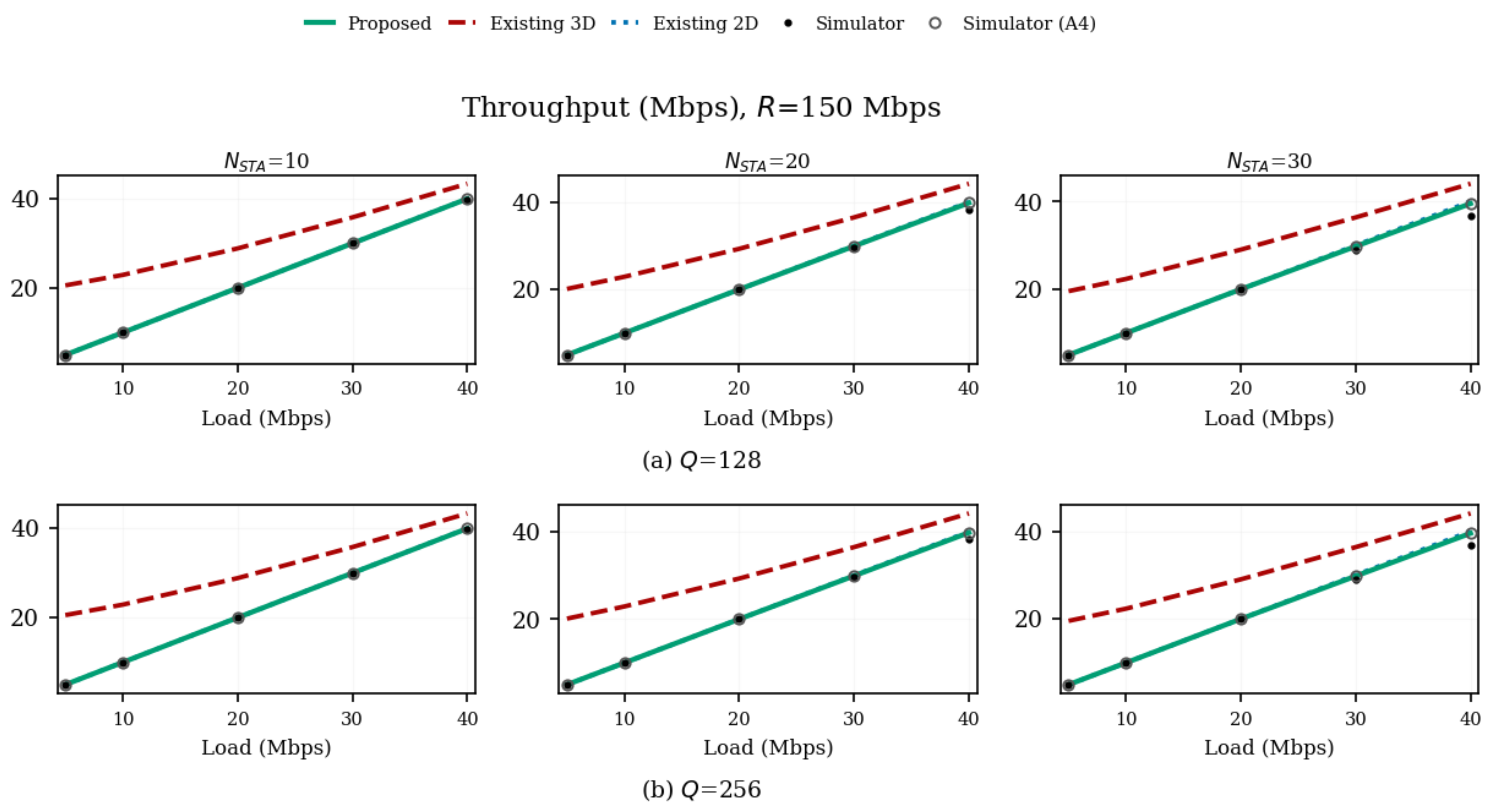
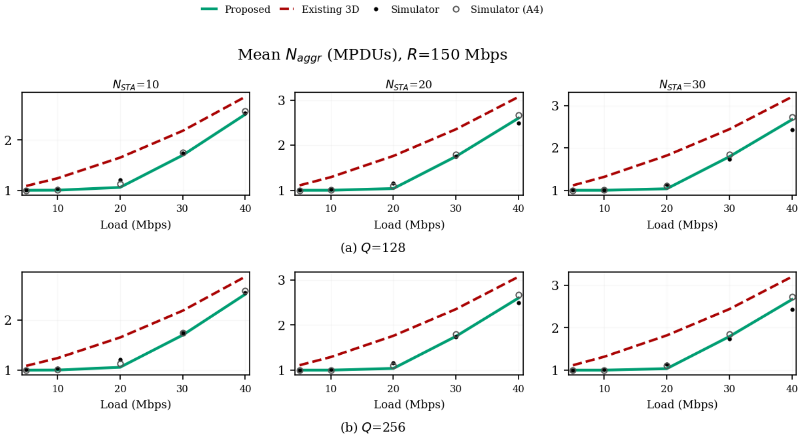
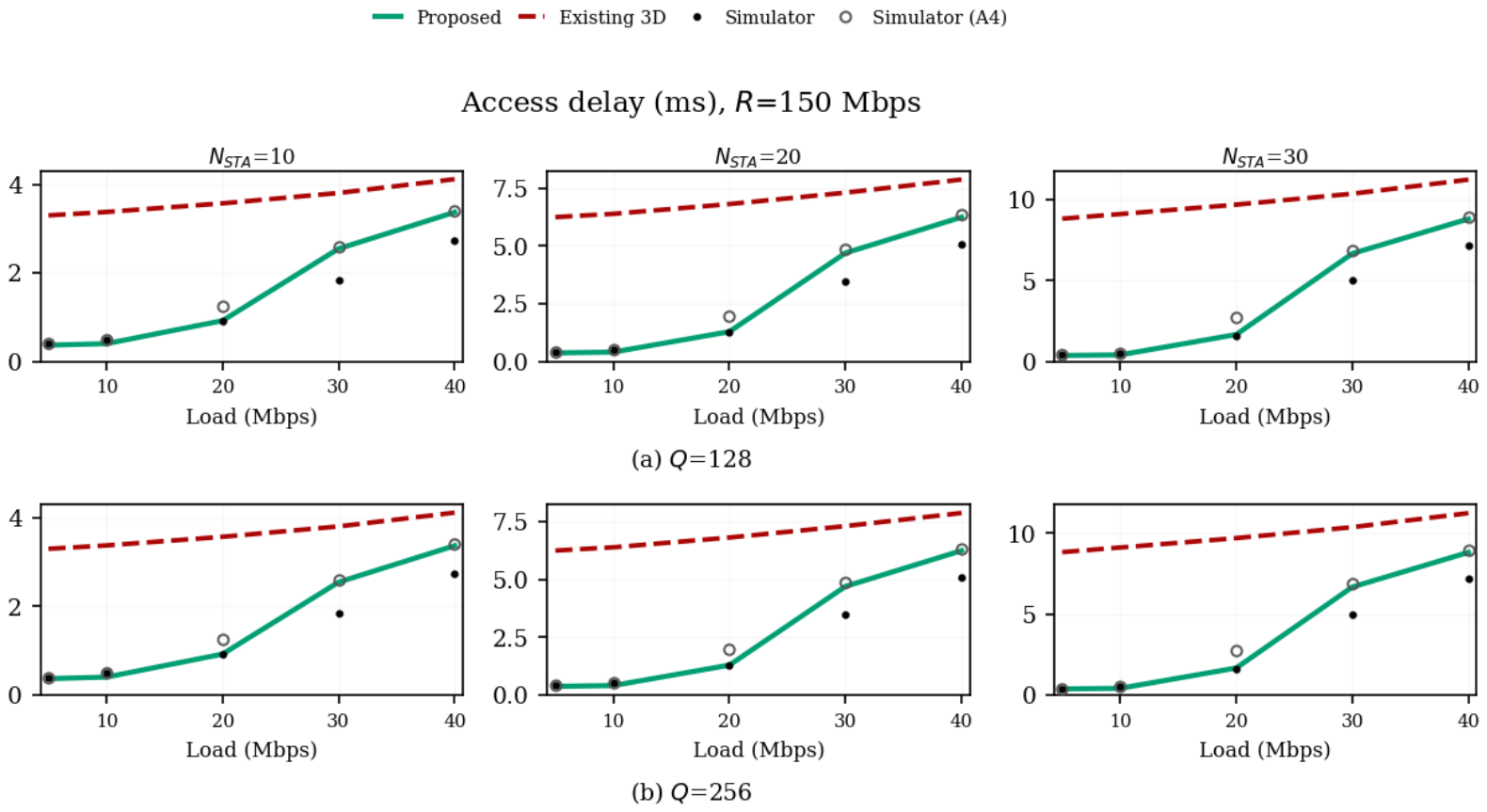
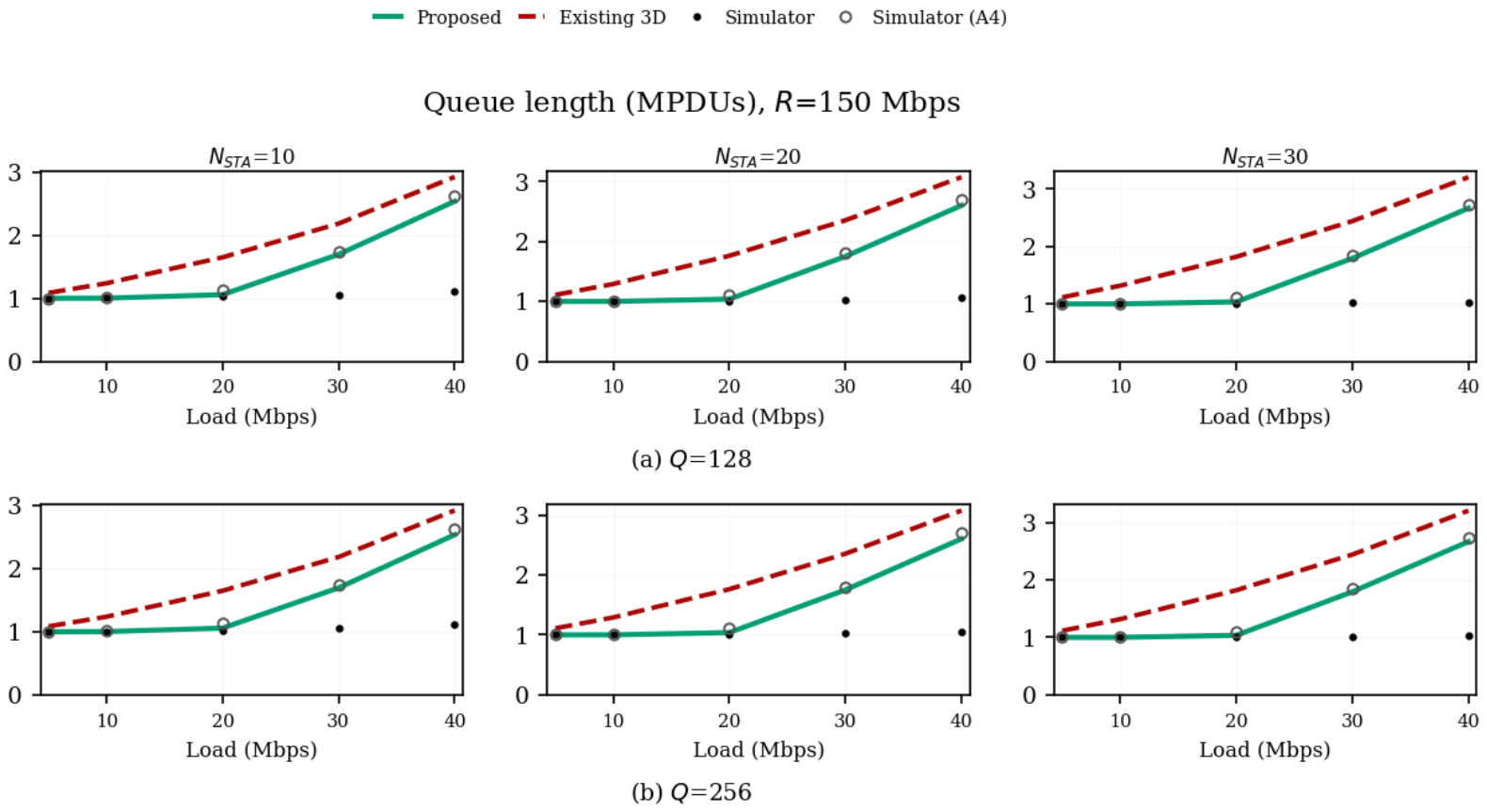
This appendix reports the same four metrics as Section 4 for an 802.11n PHY rate of R = 150 Mbps using the identical evaluation methodology (Table 2): the same two analytical baselines, the same two simulator variants, N S T A { 10 , 20 , 30 } , Q { 128 , 256 } , five seeds per point with a 1 s warm-up, and offered loads swept up to 600 Mbps. Figure A1, Figure A2, Figure A3 and Figure A4 cover the full load range, and Figure A5, Figure A6, Figure A7 and Figure A8 restrict the load to ≤40 Mbps to resolve the light-load region.
The qualitative conclusions of Section 4 carry over unchanged: the proposed model tracks the simulator closely in throughput and aggregation size across the whole load range, Existing 2D overestimates both at light-to-moderate load because it always transmits a full A = 64 aggregate, and Existing 3D departs from the simulator only at light load, where its non-empty-buffer assumption inflates every metric. The quantitative comparison between the two PHY rates is, however, informative in its own right, and it bears directly on how the aggregation limit interacts with the available bandwidth.
First, the saturation throughput at R = 150 Mbps is almost insensitive to the number of stations: at Q = 128 it is 126.3 , 125.8 , and 124.8 Mbps for N S T A = 10 , 20, and 30, a spread of only about 1 % . At R = 867 Mbps the corresponding spread is roughly three times larger ( 513.4 , 504.2 , and 495.3 Mbps). The reason is that the collision cost T c o l l is rate-independent, whereas the successful-transmission airtime shrinks as R grows; collisions therefore consume a proportionally larger share of the channel at the higher rate, making the saturation throughput more sensitive to contention.
Second, and for the same reason, a large aggregation limit is more valuable at the higher rate. At R = 150 Mbps the data portion of a 64-MPDU A-MPDU already dominates the fixed per-access overhead, so the network saturates at essentially the full aggregate regardless of N S T A ; at R = 867 Mbps the fixed overhead is comparable to the data airtime for small aggregates, so the ability to build large batches is what keeps the channel efficient. This is the practical sense in which the aggregation limit “balances” performance across bandwidths: it is a soft cap, l n = min ( A , n ) , that binds only when the backlog allows, and its benefit grows with the PHY rate.
Third, the absolute service time scales inversely with the rate as expected: near saturation at Q = 128 it is about 31.0 , 56.5 , and 75.0 ms for N S T A = 10 , 20, and 30 at R = 150 Mbps, roughly four times the corresponding values at R = 867 Mbps ( 7.6 , 14.1 , and 19.5 ms). The model reproduces these values to within a few percent of the simulator at both rates.
Figure A1. Network throughput versus offered load at R = 150 Mbps, with columns for N S T A { 10 , 20 , 30 } and rows for Q { 128 , 256 } . Curves compare the proposed model, Existing 3D [16], Existing 2D [15], the simulator, and the simulator under Assumption 4.
Futureinternet 18 00451 g0a1
Finally, the light-load figures (Figure A5, Figure A6, Figure A7 and Figure A8) make the contrast with Existing 3D explicit at R = 150 Mbps as well: over Λ 40 Mbps its throughput, aggregation size, service time, and queue length all sit visibly above the proposed model and both simulator variants because it assumes a station always has a packet to send. The proposed model, by contrast, reproduces the throughput and aggregation size of both simulator variants almost exactly in this regime and matches the assumption-matched simulator (A4) closely for the service time and queue length; the default simulator lies below the model for these two metrics because an A-MPDU that keeps aggregating during backoff clears the backlog in fewer services, which is precisely the Assumption 4 effect isolated in Section 4.4 and Section 4.5.
Figure A2. Average aggregation size N ¯ a g g r versus offered load at R = 150 Mbps in the same layout and with the same curves as Figure A1.
Futureinternet 18 00451 g0a2
Figure A3. Average MAC service time D ¯ versus offered load at R = 150 Mbps in the same layout as Figure A1 (Existing 2D is omitted as it does not model the service time).
Futureinternet 18 00451 g0a3
Figure A4. Average per-station queue length n ¯ at the A-MPDU formation instants versus offered load at R = 150 Mbps in the same layout as Figure A1 (Existing 2D is omitted as it does not model the queue).
Futureinternet 18 00451 g0a4
Figure A5. Light-load detail of the network throughput at R = 150 Mbps ( Λ 40 Mbps, far below the ≈126 Mbps saturation level) in the same layout as Figure A1.
Futureinternet 18 00451 g0a5
Figure A6. Light-load detail of the average aggregation size N ¯ a g g r at R = 150 Mbps in the same layout as Figure A1.
Futureinternet 18 00451 g0a6
Figure A7. Light-load detail of the average MAC service time D ¯ at R = 150 Mbps in the same layout as Figure A3.
Futureinternet 18 00451 g0a7
Figure A8. Light-load detail of the average per-station queue length n ¯ at R = 150 Mbps in the same layout as Figure A4.
Futureinternet 18 00451 g0a8

References

  1. Perahia, E.; Stacey, R. Next Generation Wireless LANs: 802.11 n and 802.11 ac; Cambridge University Press: Cambridge, UK, 2013. [Google Scholar]
  2. Seytnazarov, S.; Choi, J.G.; Kim, Y.T. Enhanced mathematical modeling of aggregation-enabled WLANs with compressed blockACK. IEEE Trans. Mob. Comput. 2018, 18, 1260–1273. [Google Scholar] [CrossRef] [Scilit]
  3. Bellalta, B.; Carrascosa, M.; Galati-Giordano, L.; Geraci, G. Delay Analysis of IEEE 802.11be Multi-Link Operation Under Finite Load. IEEE Wirel. Commun. Lett. 2023, 12, 595–598. [Google Scholar] [CrossRef] [Scilit]
  4. Wilhelmi, F.; Galati-Giordano, L.; Geraci, G.; Bellalta, B.; Fontanesi, G.; Nuñez, D. Throughput Analysis of IEEE 802.11bn Coordinated Spatial Reuse. In Proceedings of the 2023 IEEE Conference on Standards for Communications and Networking (CSCN), Munich, Germany, 6–8 November 2023; pp. 401–406. [Google Scholar] [CrossRef] [Scilit]
  5. Lin, Y.; Wong, V.W. WSN01-1: Frame aggregation and optimal frame size adaptation for IEEE 802.11 n WLANs. In Proceedings of the IEEE GLOBECOM 2006; IEEE: New York, NY, USA, 2006; pp. 1–6. [Google Scholar]
  6. Li, T.; Ni, Q.; Malone, D.; Leith, D.; Xiao, Y.; Turletti, T. Aggregation with fragment retransmission for very high-speed WLANs. IEEE/ACM Trans. Netw. 2009, 17, 591–604. [Google Scholar] [CrossRef] [Scilit]
  7. Hajlaoui, N.; Jabri, I.; Ben Jemaa, M. An accurate two dimensional Markov chain model for IEEE 802.11n DCF. Wirel. Netw. 2018, 24, 1019–1031. [Google Scholar] [CrossRef] [Scilit]
  8. Seytnazarov, S.; Jeong, D.G.; Jeon, W.S. Parallel PPDU transmission mechanism for wideband wireless LANs. IEEE Access 2020, 8, 198714–198729. [Google Scholar] [CrossRef] [Scilit]
  9. Jabri, I.; Mansour, K.; Al-Oqily, I.; Ezzedine, T. Enhanced characterization and modeling of A-MPDU aggregation for IEEE 802.11n WLANs. Trans. Emerg. Telecommun. Technol. 2022, 33, e4384. [Google Scholar] [CrossRef] [Scilit]
  10. Feng, K.T.; Huang, Y.Z.; Lin, J.S. Design of MAC-defined aggregated ARQ schemes for IEEE 802.11n networks. Wirel. Netw. 2011, 17, 685–699. [Google Scholar] [CrossRef] [Scilit]
  11. Lin, J.S.; Feng, K.T.; Huang, Y.Z.; Wang, L.C. Novel design and analysis of aggregated ARQ protocols for IEEE 802.11n networks. IEEE Trans. Mob. Comput. 2012, 12, 556–570. [Google Scholar] [CrossRef] [Scilit]
  12. Mansour, K.; Jabri, I.; Ezzedine, T. Revisiting the IEEE 802.11n A-MPDU retransmission scheme. IEEE Commun. Lett. 2019, 23, 1097–1100. [Google Scholar] [CrossRef] [Scilit]
  13. Kuppa, S.; Dattatreya, G. Modeling and analysis of frame aggregation in unsaturated WLANs with finite buffer stations. In Proceedings of the 2006 IEEE International Conference on Communications; IEEE: New York, NY, USA, 2006; Volume 3, pp. 967–972. [Google Scholar]
  14. Bellalta, B. A Queuing Model for the Non-continuous Frame Assembly Scheme in Finite Buffers. In Proceedings of the ASMTA; Springer: Berlin/Heidelberg, Germany, 2009; pp. 219–233. [Google Scholar]
  15. Kim, B.S.; Hwang, H.Y.; Sung, D.K. Effect of frame aggregation on the throughput performance of IEEE 802.11 n. In Proceedings of the 2008 IEEE Wireless Communications and Networking Conference; IEEE: New York, NY, USA, 2008; pp. 1740–1744. [Google Scholar]
  16. Seytnazarov, S.; Jeong, D.G.; Jeon, W.S. Performance Analysis of Aggregation-Enabled IEEE 802.11 WLANs with Variable Aggregation Size. IEEE Access 2023, 11, 119373–119387. [Google Scholar] [CrossRef] [Scilit]
  17. Seytnazarov, S.; Jeong, D.G.; Jeon, W.S. Performance analysis of IEEE 802.11 WLANs with frame aggregation and unsaturated traffic load. In Proceedings of the 2024 IEEE International Black Sea Conference on Communications and Networking (BlackSeaCom), Tbilisi, Georgia, 24–27 June 2024; pp. 165–170. [Google Scholar] [CrossRef] [Scilit]
  18. IEEE Std 802.11n-2009; Enhancements for Higher Throughput. IEEE: New York, NY, USA, 2009; pp. 1–565. [CrossRef] [Scilit]
  19. IEEE Std 802.11ac-2013; Enhancements for Very High Throughput for Operation in Bands Below 6 GHz. IEEE: New York, NY, USA, 2013; pp. 1–425. Available online: https://standards.ieee.org/ieee/802.11ac/4473/ (accessed on 11 August 2026).
  20. Seytnazarov, S.; Jeong, D.G.; Sook Jeon, W. A Simple Performance Model of IEEE 802.11 WLAN with Arbitrary Buffer Size and Traffic Load. In Proceedings of the 2024 International Conference on Information Networking (ICOIN), Ho Chi Minh City, Vietnam, 17–19 January 2024; pp. 120–125. [Google Scholar] [CrossRef] [Scilit]
  21. Behara, A.; Venkatesh, T.G. Performance Analyses of Uplink MU-OFDMA Hybrid Access MAC in IEEE 802.11ax WLANs. IEEE Syst. J. 2022, 16, 5108–5119. [Google Scholar] [CrossRef] [Scilit]
  22. Behara, A.; Venkatesh, T.G. Performance Analysis and Energy Efficiency of MU- (OFDMA & MIMO) Based Hybrid MAC Protocol of IEEE 802.11ax WLANs. IEEE Trans. Veh. Technol. 2023, 72, 6474–6490. [Google Scholar] [CrossRef] [Scilit]
  23. Meng, J.; Zhao, Q.; Wu, W.; Jin, M.; Song, P.; Liu, Y. Enhancing IEEE 802.11ax Network Performance: An Investigation and Modeling Into Multi-User Transmission. IEEE Trans. Mob. Comput. 2025, 24, 2151–2165. [Google Scholar] [CrossRef] [Scilit]
  24. Meng, J.; Deng, C.; Song, P.; Jin, M.; Liu, Y. Modeling Nonsaturated IEEE 802.11ax Networks with the Coexistence of UORA and UONRA in Imperfect Channels. IEEE Trans. Mob. Comput. 2026, 25, 4190–4205. [Google Scholar] [CrossRef] [Scilit]
  25. Magrin, D.; Avallone, S.; Roy, S.; Zorzi, M. Performance Evaluation of 802.11ax OFDMA Through Theoretical Analysis and Simulations. IEEE Trans. Wirel. Commun. 2023, 22, 5070–5083. [Google Scholar] [CrossRef] [Scilit]
  26. Bianchi, G. Performance analysis of the IEEE 802.11 distributed coordination function. IEEE J. Sel. Areas Commun. 2000, 18, 535–547. [Google Scholar] [CrossRef] [Scilit]
  27. Raptis, P.; Vitsas, V.; Paparrizos, K. Packet delay metrics for IEEE 802.11 distributed coordination function. Mob. Netw. Appl. 2009, 14, 772–781. [Google Scholar] [CrossRef] [Scilit]
  28. Seytnazarov, S. 802.11n/ac Wi-Fi Simulator. 2023. Available online: https://github.com/shinnazar/802.11n-ac-Wi-Fi-simulator (accessed on 11 August 2026).
  29. Tinnirello, I.; Bianchi, G.; Xiao, Y. Refinements on IEEE 802.11 distributed coordination function modeling approaches. IEEE Trans. Veh. Technol. 2009, 59, 1055–1067. [Google Scholar] [CrossRef] [Scilit]
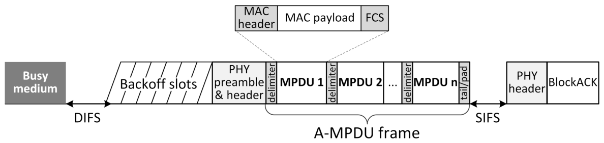
Figure 1. A-MPDU and BlockAck frames.
Futureinternet 18 00451 g001
Figure 2. Three-dimensional Markov chain of the queue size, the backoff stage, and the backoff counter.
Futureinternet 18 00451 g002
Figure 3. Network throughput versus offered load at R = 867 Mbps, with columns for N S T A { 10 , 20 , 30 } and rows for Q { 128 , 256 } . Curves compare the proposed model, Existing 3D [16], Existing 2D [15], the simulator, and the simulator under Assumption 4. Each panel includes an inset showing the light-load region ( Λ 100 Mbps, far below the ≈500 Mbps saturation level), where Existing 3D’s non-empty-buffer assumption is most visible.
Futureinternet 18 00451 g003
Figure 4. Average aggregation size N ¯ a g g r versus offered load at R = 867 Mbps in the same layout and with the same curves as Figure 3.
Futureinternet 18 00451 g004
Figure 5. Average MAC service time D ¯ versus offered load at R = 867 Mbps in the same layout as Figure 3 (Existing 2D is omitted as it does not model the service time).
Futureinternet 18 00451 g005
Figure 6. Average per-station queue length n ¯ at the A-MPDU formation instants versus offered load at R = 867 Mbps in the same layout as Figure 3 (Existing 2D is omitted as it does not model the queue).
Futureinternet 18 00451 g006
Table 1. Comparison of existing frame-aggregation performance models for IEEE 802.11 WLANs.
Model(s)Traffic LoadAggregation Size ControlContends Only If Data Present?Metrics Derived
[5,6,7,8,9]SaturatedFixed/maximumNoThroughput (delay in some works)
[2,10,11,12]SaturatedARQ-driven (channel-error-dependent)NoThroughput (delay in some works)
[13,14]UnsaturatedPredefined service-time distributionYesThroughput, delay
[15]UnsaturatedFixed at K accumulated packetsYes (only after K packets accumulate)Throughput
[16]Unsaturated (dummy-padded)Always 1 packet (dummy packet if empty)NoThroughput, aggregation size
Proposed (this work)UnsaturatedDynamic (offered load, backoff process, N S T A )YesThroughput, aggregation size, service time, queue length
Table 2. System parameters.
SymbolNameValues
AMaximum aggregation size64 packets
L h d r Link, network, and transport layer headers66 bytes
L p l d The length of the data payload800 bytes
N S T A Number of stations10, 20, and 30
QQueue capacity128 and 256 packets
RPHY data transmission rate867 Mbps (main text); 150 Mbps (Appendix A)
rRetry limit6
T B A C K BlockAck duration32 μ s
T C T S CTS duration44 μ s
T D I F S DIFS duration34 μ s
T P H Y PHY preamble and header duration40 μ s
T R T S RTS duration34 μ s
T S I F S SIFS duration16 μ s
W 0 Minimum contention window size16
W m a x Maximum contention window size1024
σ Idle slot duration9 μ s
Λ Total offered traffic load in the network50 to 3000 Mbps ( R = 867 ); 20 to 600 Mbps ( R = 150 )
Disclaimer/Publisher’s Note: The statements, opinions and data contained in all publications are solely those of the individual author(s) and contributor(s) and not of MDPI and/or the editor(s). MDPI and/or the editor(s) disclaim responsibility for any injury to people or property resulting from any ideas, methods, instructions or products referred to in the content.