Article

Intelligent Carbon-Aware Gateway Placement for Green IoT Networks

by
Francisco-Jose Alvarado-Alcon
1,2,
Rafael Asorey-Cacheda
1,2,*,
Joan Garcia-Haro
1,2 and
Antonio-Javier Garcia-Sanchez
1,2
1
Department of Information and Communication Technologies, Universidad Politécnica de Cartagena Member of European University of Technology EUT+, 30202 Cartagena, Spain
2
People Oriented Smart Technologies Laboratory, European Research Group, European University of Technology, European Union, 10004 Troyes, France
*
Author to whom correspondence should be addressed.
Future Internet 2026, 18(8), 389; https://doi.org/10.3390/fi18080389
Submission received: 6 July 2026 / Revised: 21 July 2026 / Accepted: 22 July 2026 / Published: 25 July 2026
(This article belongs to the Section Internet of Things)

Abstract

Sustainable Internet of Things (IoT) deployments require network planning strategies that explicitly account for environmental impact and not only traditional performance and energy metrics. This work analyzes how input representations affect a learning-based framework for carbon footprint (CF)-aware gateway placement in LoRa multi-hop IoT networks. Building on a previous CF model and an integer linear programming dataset, a multilayer perceptron is retrained using different input encodings: end-device coordinates, traffic-based weights, spatial sampling regions (SSRs), and a global CF estimate. Their contributions are evaluated through Shapley additive explanations (SHAP)-based explainability analysis, ablation studies, and sensitivity analysis. Results show that the CF estimate is the most influential input, acting as a global guidance signal that drives large gateway relocations. The combination of raw coordinates and SSR-based spatial summaries achieves the best performance by capturing both fine spatial detail and collective relay opportunities, while traffic-based weights mainly contribute through aggregate effects. These findings provide practical guidelines for designing CF-aware learning pipelines and offer insights to support future research on environmentally aware artificial intelligence for IoT network planning.

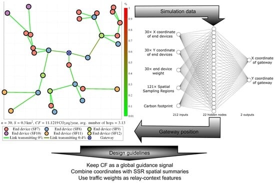
Graphical Abstract

1. Introduction

As the world moves toward more pervasive connectivity, Internet of Things (IoT) systems are central to many sectors, from precision agriculture to Industry 5.0, enabling massive sensing and automation while introducing new environmental responsibilities. Designing wireless IoT deployments requires placing many low-cost end devices across an area so that they can sample the physical world and forward data to gateways (sinks) that relay them to servers for processing. Multi-hop topologies, where end devices may forward packets on behalf of others, can dramatically extend the coverage of a single gateway and avoid the cost and energy overhead of deploying excessive gateways [1]. Thus, multi-hop operation is an attractive way to increase scalability while reducing infrastructure needs. However, configuring multi-hop networks introduces many more degrees of freedom than single-hop deployments, complicating optimization and planning.
Traditionally, optimization of such networks focused on quality of service, lifetime, throughput, or simple energy metrics. Those metrics are important, but they do not capture the full environmental impact of the network. The concept of green communications reframes network design so that the carbon footprint (i.e., the CO2 emissions associated with manufacturing, powering and maintaining communications equipment and energy sources) becomes a priority objective. By explicitly estimating and minimizing the carbon footprint (CF) of a deployment, planners can avoid solutions that are locally energy-efficient but environmentally costly over device and power-supply life cycles.
Many works evaluate network performance using simulation or exact optimization. Integer linear programming (ILP) formulations can ascertain optimal gateway placements, but they scale poorly to realistic scenarios and incur a significant computational cost, which itself has an environmental impact. Heuristics and artificial intelligence (AI) therefore constitute attractive alternatives that trade optimality for dramatically shorter runtime and lower carbon costs. For LoRaWAN networks, an ILP formulation for joint gateway placement and configuration was proposed in [2]; the authors compared exact solutions with heuristic approximations and observed that a greedy heuristic yielded competitive results, whereas a genetic algorithm (a search heuristic inspired by natural evolution) failed to recover a good approximation of the Pareto front. A similar comparison among ILP, reinforcement learning (RL), and deep supervised learning for drone-assisted cellular coverage appears in [3]: the ILP found the true optimum but required substantially more computation (and thus greater carbon expenditure), while a deep model approached optimal performance and RL did not yield comparable results. Importantly, the inference cost of the AI models was negligible relative to solving the ILP, making them appealing for fast, green decision-making. Similarly, a work by Maddikunta et al. [4] used heuristics to optimize energy in cluster networks by head selection. Drone coverage for LoRaWAN was considered in [5].
However, one practical difficulty for AI-based methods is the large variety of ways to represent network state: input encoding can produce significant differences in predictive quality and generalization. Creative encodings can therefore meaningfully improve model performance, as illustrated in [6], where a Coulomb’s law–inspired encoding that computes a “force” for each device based on its degree and that of its neighbors is used to identify influential end devices, after which the force-to-throughput ratio is evaluated using the NS-3 simulator.
In [7], following this line of work, we developed a complete CF estimation model and an ILP formulation to minimize this environmental footprint of LoRa-based multi-hop networks (including photovoltaic power and battery life-cycle emissions) and showed large CF benefits from having end devices forward traffic instead of blindly increasing gateway counts. Building on that modeling effort, we later showed that machine learning models can approximate the results of ILP with orders of magnitude less computational cost, enabling fast, scalable green planning; the multilayer perceptron (MLP)-based workflow achieved substantial CF reductions (MLP 14 % reduction vs. unoptimized placement; ILP 16.6 % ), while greatly lowering computation time and its environmental cost [8].
The present paper builds on our previous work [7,8,9] but shifts the focus from optimization performance to model understanding. Specifically, we investigate what information a neural model actually needs, how different input encodings affect its behavior, and which feature groups provide transferable insight for the design of CF-aware learning pipelines. In particular, we analyze the roles of raw coordinates, traffic-based weights, spatial sampling regions (SSRs), and an intermediate CF estimate through complementary explainability tools. Two recurring practical issues motivate this study: (i) real deployments often provide only unordered sets of device positions (a point cloud) rather than fixed, ordered vectors, and (ii) planners may wish to adapt a trained workflow to new scenarios (e.g., adding drone relays to temporarily augment capacity instead of over-dimensioning ground infrastructure).
The concept of understanding the behavior of artificial intelligence models is commonly referred to as explainable artificial intelligence (XAI). Such understanding can support better model design; facilitate model improvement; and enhance trust, reliability, and robustness [10,11,12,13,14]. Although XAI has attracted growing interest in several application domains, its adoption in telecommunications remains comparatively limited. Existing works range from low-level wireless communications, where explainability is used to improve link performance [10], to network-level tasks such as failure identification [11].
The proposed explainability-oriented analysis provides scientific insight beyond the performance results reported in our earlier optimization studies. It shows how permutation invariance can emerge in a standard MLP trained with unordered end device inputs, how CF acts as a global descriptor of the improvement margin rather than as a direct location cue, and why coarse spatial summaries such as SSRs can be important even when their marginal Shapley additive explanations (SHAP) scores are relatively small. These findings clarify the respective roles of global environmental descriptors and local spatial encodings, thereby informing the design of scalable and interpretable green IoT planning methods.
The main contributions of this paper are the following:
  • A complete analysis of the trained MLP weights and activations to understand how the network uses an unordered set of end device positions (point-cloud-style inputs) to predict gateway placement for CF reduction.
  • An importance analysis identifying the most influential input information for green gateway placement. This analysis is intended to guide future model design and data-collection priorities.
  • Design guidelines for CF-aware learning-based network planning, illustrating how the same CF-aware framework can support dynamic and hybrid green deployments.
The remainder of the paper is organized as follows. Section 2 summarizes the CF model and ILP used to generate ground truth, and it also details the MLP architectures and input encodings we analyze. Section 3 presents the weight and importance analyses. Section 4 concludes the paper with guidelines for green network planning.

2. Materials and Methods

To provide network coverage, gateways must be placed such that they can communicate with end devices. Therefore, the number and positions of the gateways are critical design factors. Additionally, the intended recipient, or next hop, and the configuration of each link must be selected. This work reuses the network and carbon footprint model introduced in [7]; all calculations and scenario parameters are identical to that work. For each scenario, the total CF is computed as the sum of gateway and end-device life cycle contributions, including operational electricity consumption provided by photovoltaic panels and battery life-cycle emissions. Manufacturing and end-of-life emissions are not optimized in this study, as the number of end devices is assumed to be constant across all scenarios. We train a new MLP based on the second architecture from [8] using the same dataset, and we repeat the full training procedure. All computational experiments and analyses reported in this work were performed using MATLAB R2024a.

2.1. Network Model

LoRa is a widely used physical (PHY) layer technology for low-power wide-area networks (LPWANs), designed to enable long-range and low-power communications by employing chirp spread spectrum (CSS) modulation. In CSS, information is conveyed through chirps whose instantaneous frequency sweeps across a given bandwidth, which provides high robustness to noise and enables reception at low signal-to-noise ratios. LoRa links are typically configured through a small set of PHY parameters, among which the spreading factor (SF) is the most influential in coverage and airtime: increasing SF increases receiver sensitivity (hence improving range) but decreases the data rate and increases time on air, directly affecting energy consumption and channel occupancy. Consequently, SF selection trades throughput and energy against robustness and coverage [15]. Because LoRa commonly operates in unlicensed sub-gigahertz bands, regulatory constraints limit channel occupancy. In the European frequency band of 868 M Hz , a widely used constraint is a 1% maximum duty cycle per sub-band.
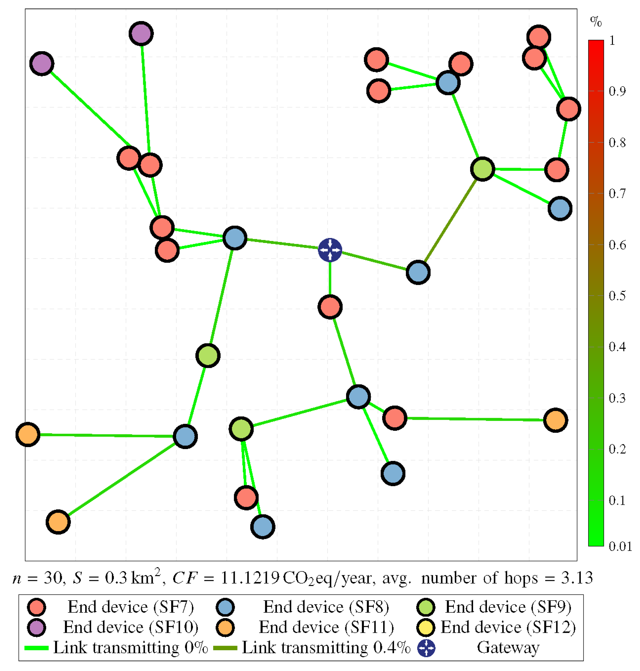
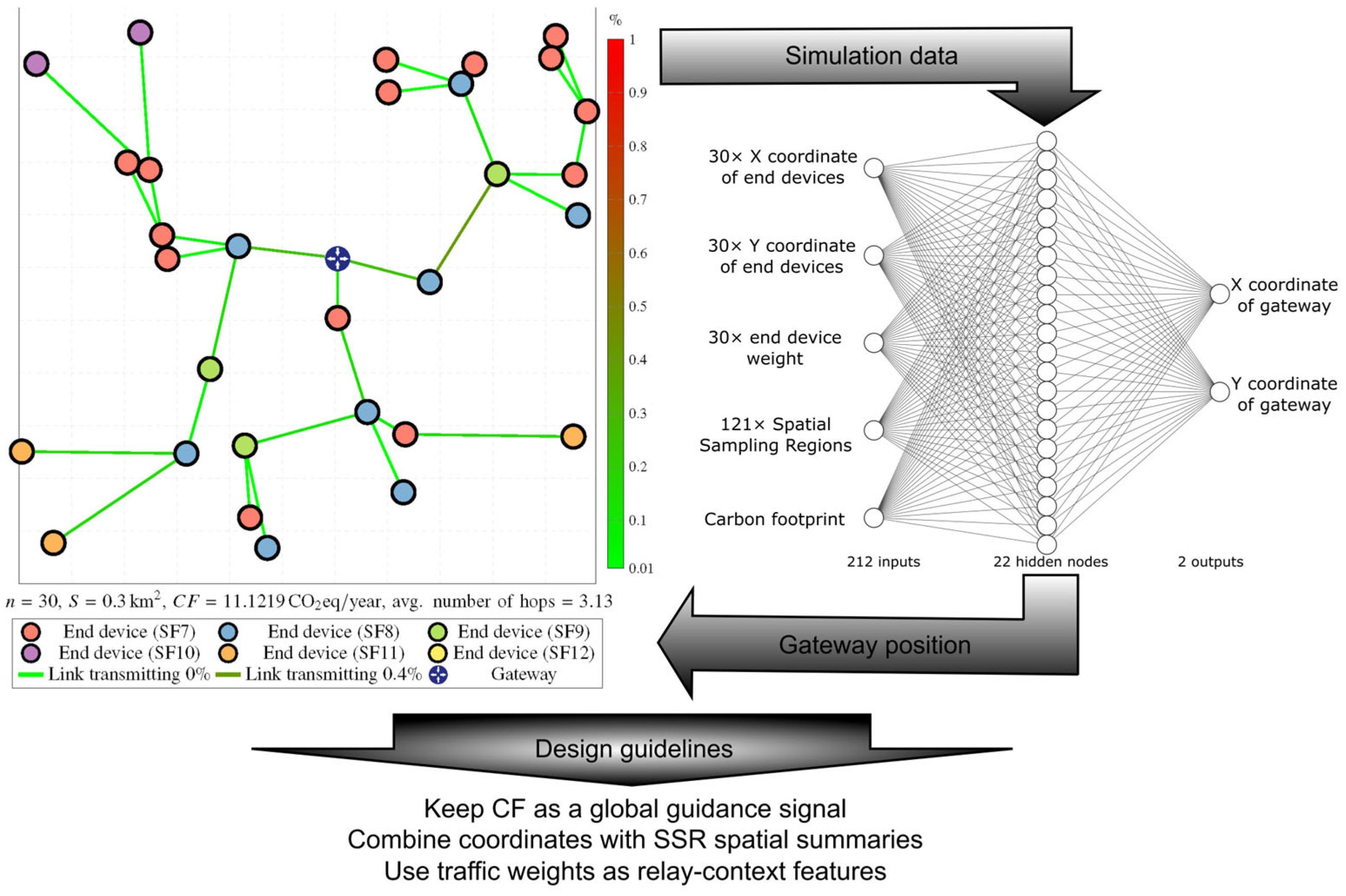
Although LoRaWAN, the standard protocol for LoRa, natively only supports star-of-stars deployments, here the physical LoRa layer is used within a multi-hop topology. We adopt the LoRa-based multi-hop model from [7]: end devices may forward received packets during predefined time slots until the packet reaches a gateway. End devices are preprogrammed with knowledge of their next hop, and the effect of clock drift or collisions is sufficiently small to be disregarded. A typical scenario (illustrated in Figure 1) places n = 30 end devices uniformly at random within an urban square area with area S =   0.3  km2. Although LoRa links can span tens of kilometers in rural environments, measurement campaigns show a significant degradation of the packet delivery ratio in urban settings [5]. Under the adopted propagation and interference model, this area represents the largest urban region for which a single gateway can still provide near-complete coverage, making it a suitable test case to study multi-hop operation and CF-aware gateway placement. End devices generate identical uplink traffic (10 packets/ h of 250 bits), and radios use the same maximum transmission power (14 dBm). This multi-hop topology was shown to have a positive impact on the CF of the proposed network compared to classic LoRaWAN topologies [7].
The problem of placement and configuration is modeled as an integer linear program. Gateway locations are discretized as an array of K candidate points on the plane, P = { ( x k , y k ) } k = 1 K , and each point may host a gateway ( G k = 1 ) or remain empty ( G k = 0 ). Binary and integer decision variables encode (i) gateway deployment over P via { G k } , (ii) the next hop chosen for an end device (to another end device or a deployed gateway), and (iii) SF assignment per link. The objective minimizes the carbon footprint computed by the life-cycle model subject to connectivity, duty-cycle, and link feasibility constraints. Link feasibility captures the requirement that the received signal conditions under the selected SF satisfy the adopted propagation model, while the duty-cycle constraints ensure that the total airtime induced by both a device’s own traffic and forwarded traffic does not violate the regulatory maximum occupancy. The ILP therefore yields ground-truth gateway placements and the corresponding configuration used to label training samples in [8].
For experiments where the gateway location is known (e.g., the position is calculated by the MLP), we use a simplified ILP formulation with fixed gateway positions (i.e., fixing the selected elements of { G k } to match the predicted coordinates after discretization) and solve the ILP to obtain feasible next-hop and SF assignments and to evaluate the CF of the MLP-predicted solution. As part of this evaluation, the ILP also determines the per-device forwarding load, which is used to compute the corresponding traffic weights. This hybrid workflow preserves comparability with the ILP-optimized baseline while exploiting the MLP for rapid gateway selection.

2.2. Carbon Footprint

We quantify the network CF using the same life-cycle accounting adopted in [7,8]. The total network footprint is computed by combining gateway and end-device contributions while keeping the number of end devices fixed across scenarios (such that their manufacturing/end-of-life contributions do not influence the optimization process).
Gateway energy consumption is modeled according to the gateway analysis in [16]. To remain conservative, we use the worst-case configuration among those analyzed: a Lorrier LR2 gateway with Long-Term Evolution (LTE) backhaul.
End-device consumption is driven by the time on air required to deliver traffic and by listening for an acknowledgment. Both terms depend on the amount of transmitted traffic and the selected SF (higher SF increases time on air), and therefore multi-hop forwarding can substantially change the per-device energy profile.
End devices and gateways are powered by photovoltaics and include a battery with enough capacity for 24 h of operation. Thus, we convert energy demands into CF through two life-cycle scalar factors: K P , capturing the photovoltaic-panel contribution, and K B , capturing the battery contribution associated with daily cycling (365 recharge cycles/year for a battery with enough capacity to power the device for 24 h). The end-device CF is then obtained by applying the combined K P + K B factor to each device’s energy consumption. The total CF of the network, C T , is the sum of the CF of all end devices and gateways.

2.3. Integer Linear Programming Formulation

Using the network and CF models defined above, the gateway placement and configuration problem is formulated as an ILP problem that minimizes the total network carbon footprint, following the formulation introduced in [7]. The objective value C T is computed from the gateway and end-device energy terms defined in the CF model; link-dependent energy and airtime parameters are precomputed for feasible links and for the selected SF configuration so that infeasible links can be excluded from the candidate set. The parameters and decision variables are summarized in Table 1.
minimize C T
subject to k = 1 p L i , k + j = 1 n L N i , j j = 1 n L N j , i = 1 , i N ,
i = 1 n L i , k α G k , k P ,
k = 1 p L i , k P T x i , k + j = 1 n L N i , j P T N x i , j 0.01 , i N ,
L i , k N 0 , i N , k P ,
L N i , j N 0 , i N , j N ,
G k { 0 , 1 } , k P .
Constraint (2) enforces flow conservation, ensuring that each end device injects one unit of generated traffic and that relayed traffic is consistently forwarded until it reaches a gateway. Constraint (3) allows traffic to be delivered to a candidate point only if a gateway is deployed there. Constraint (4) imposes the 1% duty-cycle limitation on each end device, accounting for both its own transmissions and forwarded traffic. Finally, constraints (5)–(7) define the domains of the integer traffic-flow variables and binary gateway-deployment variables.

2.4. Neural Network Architecture and Training

Following the two-stage workflow introduced in [8], we proceed as follows. First, a dataset of 24,000 scenario instances is generated by solving the full ILP problem defined in the previous Section 2.3, which yields ground-truth gateway placements and feasible network configurations. Next, a first-stage MLP—which does not require CF or traffic-weight features—is trained to predict the gateway position from end-device locations only. Given this initial gateway position, we solve a streamlined version of the ILP problem in which the gateway placement G k is fixed and therefore no longer optimized; as a result, this reduced formulation only needs to determine a feasible communication configuration. The network generated with this gateway position is then used to construct the input features of the second-stage MLP:
(1) and (2) Raw end-device (point-cloud) features. Each scenario is represented as an unordered set of end-device feature vectors containing (1) Cartesian coordinates ( x , y ) and (2) a weight term. Device positions are randomly generated, while transmitted traffic is computed after the first-stage network is configured by solving the streamlined ILP problem. The weight is defined as the logarithm of the transmitted traffic expressed in ‘traffic units’, where one traffic unit corresponds to the quantity of data generated by a single end device in one hour. Consequently, the weight ranges from log ( 1 ) for devices that only transmit their own traffic to log ( 30 ) for devices that also forward the traffic of the other 29 end devices.
(3) Spatial sampling regions (SSRs). To obtain a fixed-length spatial representation, the deployment area is partitioned into overlapping circular regions of radius r = 50   m , with region centers arranged on an 11 × 11 grid and inter-center distance r. This radius was selected empirically based on validation performance. Although this value achieved the best mean result among the tested radii, the confidence intervals overlapped across the evaluated values, indicating that the model is not highly sensitive to moderate changes in the SSR radius. Therefore, r = 50   m should be interpreted as a robust empirical choice rather than as a uniquely optimal value. For each SSR, the number of end devices within the region is counted, yielding a 121-dimensional spatial summary that preserves coarse locality while remaining invariant to the ordering and exact number of end devices.
(4) Carbon footprint (CF). In addition to being the optimization objective, the CF value is provided as a single scenario-level input feature. It is calculated as the sum of the CFs generated by all gateways and end devices, as described in Section 2.2. This scalar acts as a compact global descriptor of the deployment, complementing the fine-grained spatial encodings and potentially improving generalization across scenarios with different energy and infrastructure characteristics.
These four input types are used for training a second-stage MLP, which is the focus of this work and produces the final gateway placement. Table 2 reports the number, range, normalized range, mean, standard deviation, and median of each input type. The resulting dataset is split into training/validation/test subsets with proportions of 67%/17%/17%, respectively. Rare instances for which the ILP has no feasible solution with a single gateway are discarded. All inputs are min–max scaled using statistics computed on the training and validation sets (the normalized ranges shown in Table 2 correspond to the test subset and therefore do not always span the entire range [ 0 , 1 ] ).
Although all input types exhibit different statistical distributions, a key structural distinction is that the coordinate and weight features originate from an unordered set of 30 end devices. As a result, any permutation of these inputs should not affect the predicted gateway placement. To improve robustness and encourage permutation invariance for the unordered set of end devices, we apply two data augmentations: random permutations of the end-device ordering and global geometric transformations of the deployment (mirror reflections). This expected permutation symmetry and its effect on the MLP’s behavior are examined below in Section 3.1.
The second-stage MLP feeds a fixed-length input vector to a single dense hidden layer with 22 neurons, and a two-neuron output regresses gateway Cartesian coordinates. Training uses the Levenberg–Marquardt optimizer with damping parameter μ = 10 3 , mean squared error (MSE) loss and up to 1000 epochs with early stopping (patience 6). Finally, for each gateway position predicted by the second-stage MLP, the streamlined ILP problem is solved again to obtain the associated configuration and to evaluate the resulting CF.
After the MLP outputs the gateway coordinates, we follow the evaluation pipeline introduced in [8]. Specifically, the streamlined version of the ILP problem is solved with the gateway position fixed to the predicted coordinates. This step determines feasible link establishment and SF assignments and is used to compute the resulting CF. If the solution with a single gateway is infeasible, additional gateways are progressively deployed following a regular grid pattern: first two gateways, then four, and finally nine, until a feasible solution is obtained.
It should be noted that the MLP is trained using network instances whose size was selected during the ILP design phase to be close to the coverage limit of a single gateway, with only a small percentage of infeasible topologies. As discussed in [8], extending this approach to larger deployments that require multiple gateways does not necessarily require retraining an MLP to output multiple gateway positions. Instead, the set of end devices can first be partitioned into spatial clusters using standard clustering techniques (e.g., Fuzzy C-Means), after which the proposed MLP can be applied independently to each cluster to determine suitable gateway locations.
This divide-and-conquer strategy is naturally scalable because each cluster preserves the single-gateway formulation for which the model was designed, while the per-cluster predictions can be computed independently and, if required, in parallel. In this context, the main scalability limitation does not arise from the MLP itself, whose number of parameters grows linearly with the number of end devices for a fixed hidden-layer size, but from the ILP used to generate labels and evaluate configurations: as the number of end devices, candidate gateway locations, and feasible links increases, the number of decision variables and constraints grows rapidly, and the corresponding solution time becomes the dominant computational bottleneck. Therefore, constraining the optimization to local clusters is not only a practical way to address multi-gateway deployments but also a principled mechanism to maintain tractable label generation while preserving the interpretability of the learned input roles. This clustered formulation assumes that most relay interactions remain predominantly local; if strong inter-cluster dependencies arise, a second refinement step can be applied to jointly adjust neighboring gateway positions after the per-cluster initialization.

2.5. Machine Learning Explainability

Beyond predictive accuracy, the objective of this work is to provide insight into how the proposed learning model exploits input information to reduce the carbon footprint of LoRa-based multi-hop networks. XAI emphasizes that understanding data-driven models can support better training and model selection, help detect biases, and improve robustness assessments. Moreover, domain knowledge and explainability are often viewed as necessary ingredients to achieve scientific consistency and to obtain scientifically meaningful outcomes beyond raw predictive performance [12,13].
In this sense, our approach aligns with perspectives on explainable machine learning for scientific discovery, where the goal is not only to justify individual predictions but also to understand the mechanisms by which a model encodes and uses domain-relevant information. While much of the explainability literature focuses on pattern recognition and computer vision, similar principles apply to MLPs: explainability tools can identify influential input features, assess robustness to perturbations in the input data, and support human understanding of model behavior, ultimately enabling iterative model improvement [13,17]. Accordingly, we address explainability through a combination of transparent design choices, post hoc interpretability analyses, and domain-informed feature engineering, following the terminology in [12].
Interpretability in our framework is assessed through complementary importance analyses, including sensitivity analysis, ablation studies, and SHAP values [18]. Together, these methods provide insight into the contribution of each input block to the predicted gateway position, both locally and globally. In particular, they help identify the information on which the model relies and clarify how different encodings interact when optimizing the carbon footprint. Since each technique captures different aspects of model behavior, their combined use provides a more robust interpretation than any single method alone.
Feature selection methods are commonly categorized based on whether the selection criterion depends on the predictive model (wrapper approaches) or is model-agnostic (filter approaches). Although filtering is typically less computationally intensive, it may ignore feature interactions and may not reflect how features behave within the chosen learning algorithm; moreover, many filter criteria rely on simple linear relationships that can be insufficient for nonlinear models [19]. We extend this reasoning to feature importance and employ multiple wrapper-style analyses to determine which information is most relevant for CF-aware gateway placement. While the relative importance of features can vary across datasets, architectures, and network sizes, the methodological conclusions regarding which types of information are informative for the task can guide the design of sustainable IoT planning pipelines; broader implications are discussed in Section 4. Although numerical importance rankings may vary with architecture capacity and deployment density, the identified roles of global descriptors (e.g., CF-like signals) versus spatial encodings (fine coordinates and coarse summaries) are expected to remain informative across a broad class of regression-based gateway placement models.
From an optimization standpoint, the use of an MSE loss function contributes to the interpretability of the training objective: because the model outputs gateway coordinates, minimizing the MSE corresponds to minimizing the squared Euclidean distance between predicted and target gateway positions. This establishes a direct geometric relationship between loss reduction and spatial accuracy, making training progress easy to relate to the underlying placement problem.
A further element supporting explainability is the symmetry analysis presented in Section 3.1. End-device information is naturally represented as an unordered set; therefore, the predictive function should be invariant to permutations of the input ordering. By analyzing the trained weights, we study how symmetry constraints induced by data augmentation are reflected in the learned parameters. This provides a model-internal view of how a standard MLP can approximate set-like behavior without specialized set architectures, thereby increasing confidence in generalization.
Finally, domain knowledge is explicitly incorporated through the use of SSRs as input features. SSRs exploit the approximately circular nature of wireless coverage regions and provide a structured spatial summary consistent with the geometry of the deployment area. Based on insights from our previous ILP-based optimization, we expected the effective SSR radius to be on the order of the coverage radius associated with spreading factor 7, which was frequently preferred by the optimization process [7]. The final radius is selected empirically by testing multiple values and choosing the one that minimizes the validation-set carbon footprint, following a data-driven procedure analogous to selecting other hyperparameters (e.g., the number of hidden neurons). This combination of physical intuition and empirical validation illustrates how informed feature design can support both performance and interpretability.
Overall, rather than treating the neural network as a black box, this work leverages interpretability tools, symmetry considerations, and domain knowledge to explain how and why the model behaves as it does. In doing so, we aim not only to improve gateway placement recommendations but also to advance understanding of how learning-based methods can be reliably applied to green communication network design.


3. Results

We first study how the MLP handles the permutation symmetry of unordered end-device inputs in Section 3.1. Then we quantify the contribution of each input type to the MLP’s predictions using several importance analyses in Section 3.2 to understand the importance of each encoding to CF optimization.

3.1. Symmetry

The first two input types, coordinates and weights, form an unordered set of n elements, with each element having three ordered values (X-coordinate, Y-coordinate, and weight), i.e., a point cloud. A unique challenge posed by point-cloud data is the need for symmetry, meaning that the model must remain invariant to the order of the inputs. There are three main approaches to address this: sorting the input into a canonical order, enhancing the training data with various permutations, or employing a symmetric function to aggregate information from each point [20]. In our work, we use the second approach, since it integrates seamlessly with our MLP architecture while preserving compatibility with non-set inputs. This method achieves a high degree of symmetry with a relatively small number of permutations, although for a network with n unordered elements, n ! permutations could be applied.
In an MLP, each neuron computes a weighted sum of its inputs. Therefore, if two inputs have identical or nearly identical weights, swapping them produces little or no change in the output. Applying this principle, if the weights associated with the 30 X-coordinates, the 30 Y-coordinates, and the 30 traffic weights are similar within each block, the network is expected to be robust to permutations of the end-device order.
To quantify how the trained MLP respects permutation symmetry, we inspect the trained weights. Let the weight between input i and hidden layer node j be denoted as w i , j , and let the weight between hidden layer node j and output k be denoted as h j , k . For a block of n permutable inputs (e.g., the 30 X-coordinates), we compute the variability of the weights w across hidden nodes with the mean standard deviation (SD), calculated as shown in Equation (8), where h is the number of nodes in the hidden layer and w ¯ j is the average weight, computed according to Equation (9). We obtain mean SDs of 0.02 and 0.06 for the coordinates and end device weights, respectively. These values are 102 and 31 times smaller than the mean SD of the non-permutable inputs, which leads to minimal variation in the outputs when the inputs are permuted. In other words, swapping two end devices produces a negligible change at the first layer, which supports effective permutation invariance induced by augmentation.
Mean SD = 1 h j = 1 h 1 n i n w i , j w ¯ j 2
w ¯ j = 1 n i n w i , j
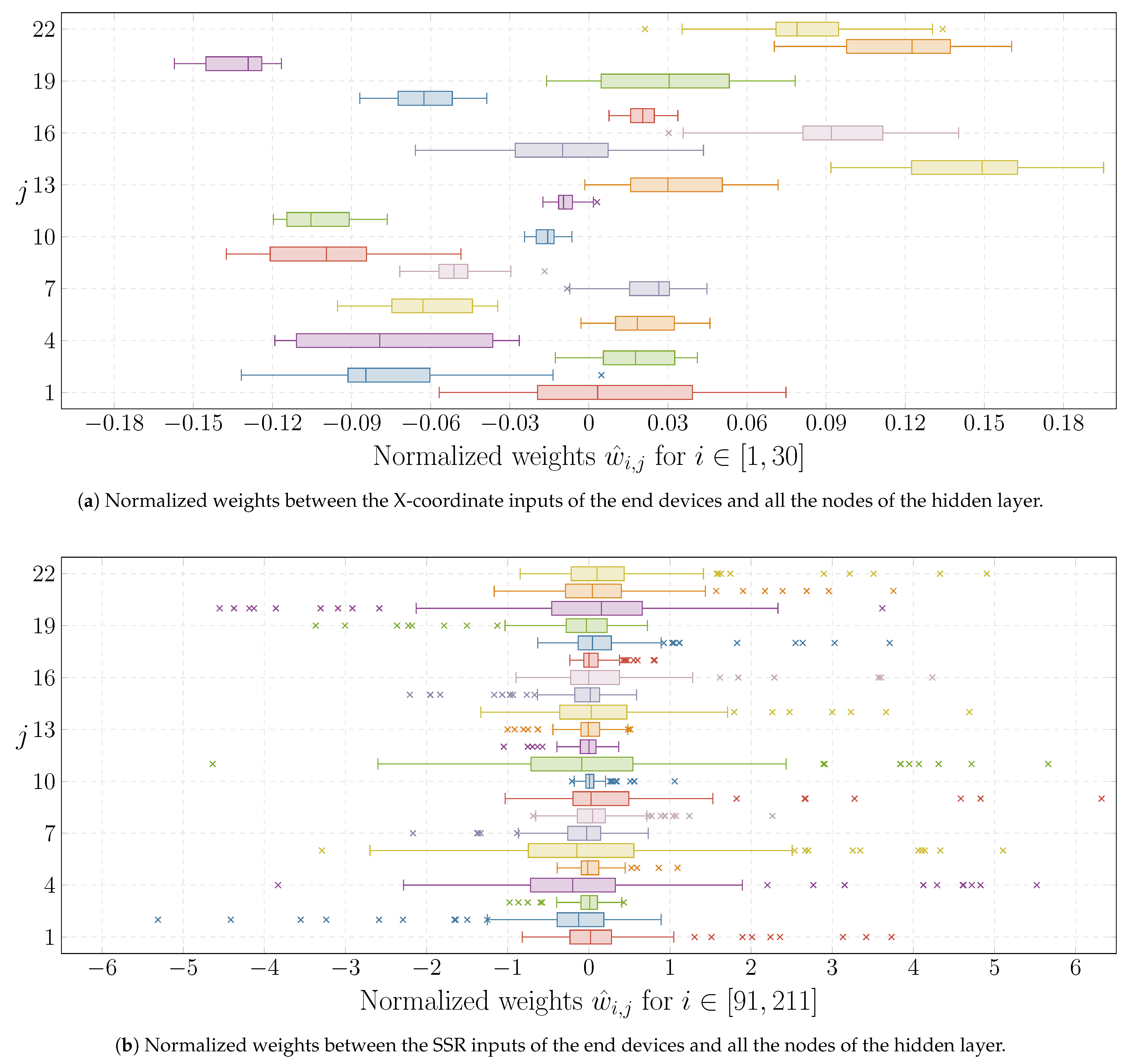
Figure 2 contrasts normalized weight distributions: Figure 2a shows w ^ i , j for the 30 X-coordinate inputs, while Figure 2b shows w ^ i , j for the 121 SSR features. The normalization, which only stretches or compacts the boxes without modifying their proportions, is achieved by multiplying w i , j by the average output weight of hidden node j as shown in Equation (10). This compensates for the different outgoing influence of hidden nodes and makes the two panels directly comparable, as some hidden nodes have weights up to 99 times higher than others.
w ^ i , j = w i , j · 1 2 k = 1 2 | h j , k |
Perfect permutation symmetry would be achieved if, for each hidden node j, all weights w i , j associated with a permutable input block were identical; in that case, any permutation of the inputs would leave the network output unchanged. In Figure 2b, which corresponds to permutation-sensitive inputs, the weights connected to each hidden node are approximately centered around zero, with zero lying between the first and third quartiles for all 22 hidden nodes, but with widely varying ranges. This behavior is expected for the SSR block, which is permutation-sensitive by design and therefore exhibits substantial per-feature variability. It should be noted that SSRs obey a global symmetry: when the entire spatial configuration is flipped or rotated, the predicted gateway position undergoes the same transformation. This global equivariance, however, is fundamentally different from element permutation invariance.
In contrast, the weights shown in Figure 2a display markedly different characteristics: zero falls within the interquartile range for only two out of the 22 hidden nodes, medians vary across nodes, whiskers are comparatively short, and outliers are rare. This concentration and consistency indicate that the coordinate block effectively behaves as an unordered set input, with individual coordinate entries being multiplied by nearly identical weights. As a result, permutations of the coordinate inputs produce negligible changes in the network output, confirming that the MLP has learned an approximate representation of end-device positions invariant to permutation.

3.2. Importance Analysis

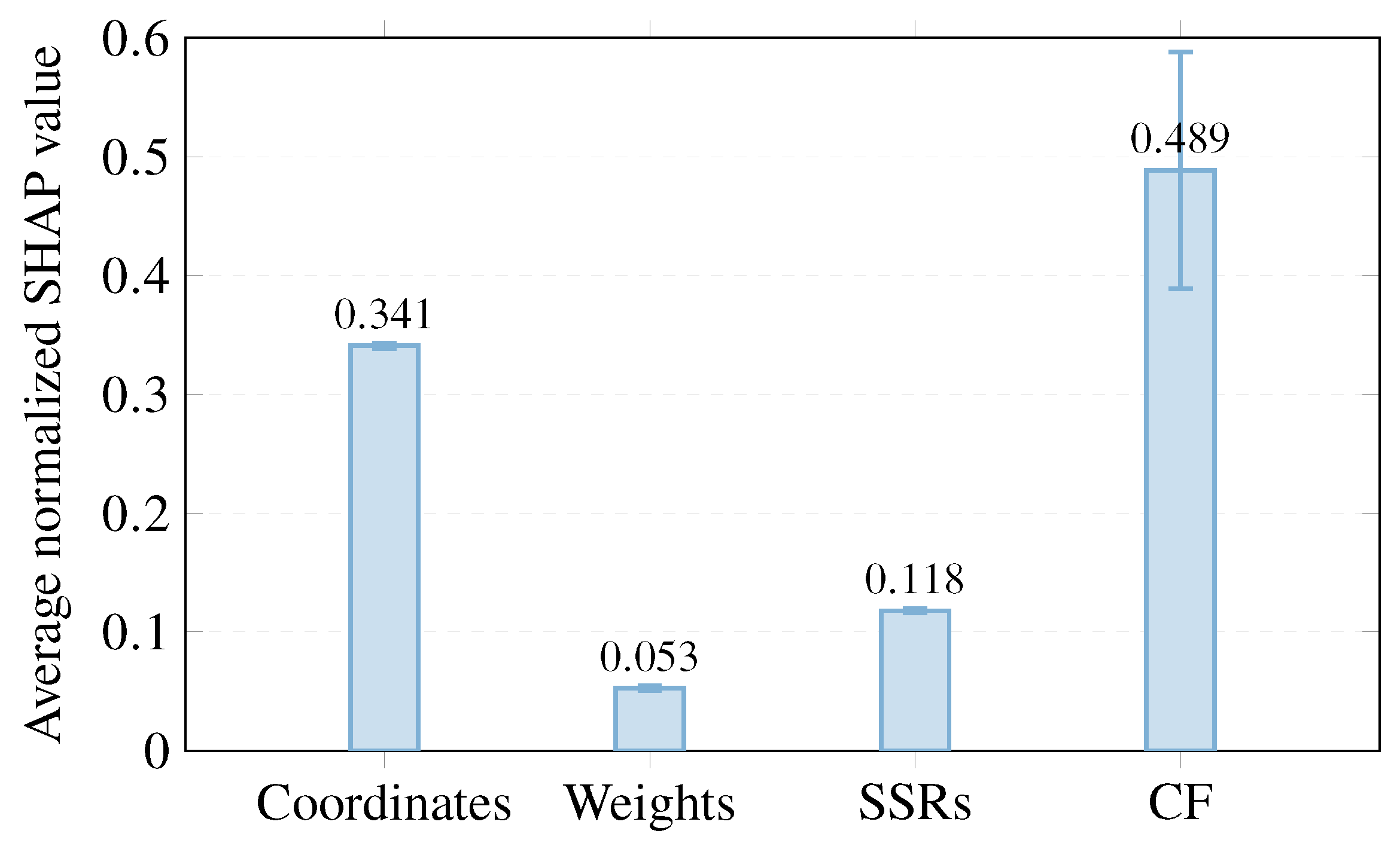
We estimate input importance with complementary methods, namely, SHAP [18] value aggregation, ablation, and sensitivity; all results are calculated on the test dataset. Figure 3 reports normalized absolute SHAP values (normalized per explained sample so that the attributions sum to one) averaged by input category (Cartesian coordinates, end-device weights, SSRs, and CF). We use 200 background test samples for the kernel SHAP approximation, and we aggregate explanations over 500 random test samples; SHAP values are computed for each output coordinate and then averaged. Error bars represent 95% bootstrap confidence intervals (1000 resamples).
SHAP analysis shows that coordinates and CF carry the largest marginal attributions, while SSRs and end-device weights have lower per-feature SHAP scores. Pairwise comparisons show that the mean absolute SHAP value of CF is significantly greater than those of coordinates, weights, and SSRs (all one-sided paired t-tests, p < 0.002), with bootstrap 95% confidence intervals for the mean differences excluding zero in all cases, as reported in Table 3.
Ablation reveals a complementary picture: replacing each input block with its median (one block at a time) produces average output differences of 0.037 (coordinates), 0.002 (weights), 0.023 (SSRs), and 0.393 (CF). These values confirm that CF is the single most influential input, but they also show that SSRs collectively have an importance comparable to raw coordinates despite low marginal SHAP scores. This aligns with the ablation study from [8], which found that training the network without the SSR inputs did not improve the CF. This apparent contradiction between SHAP and ablation arises because SSRs are a distributed, highly correlated encoding with spatial overlap: each SSR bin contributes a small marginal effect, but together, they carry a large, synergistic signal that SHAP (which attributes marginal effects) can underestimate. This is because kernel SHAP relies on perturbation-based approximations that do not fully account for dependencies among correlated inputs; therefore, it may underestimate the importance of distributed spatial encodings when interpreted in isolation [21]. The ablation experiment (which removes the collective signal) exposes this dependency, highlighting that correlated spatial encodings should be assessed at the block level before being discarded. For the CF input, the sensitivity analysis leads to a different but consistent interpretation. Unlike coordinates and SSRs, which provide local geometric information, CF is a scalar global descriptor of the network state. The effect of perturbing this value is examined in the sensitivity analysis below.
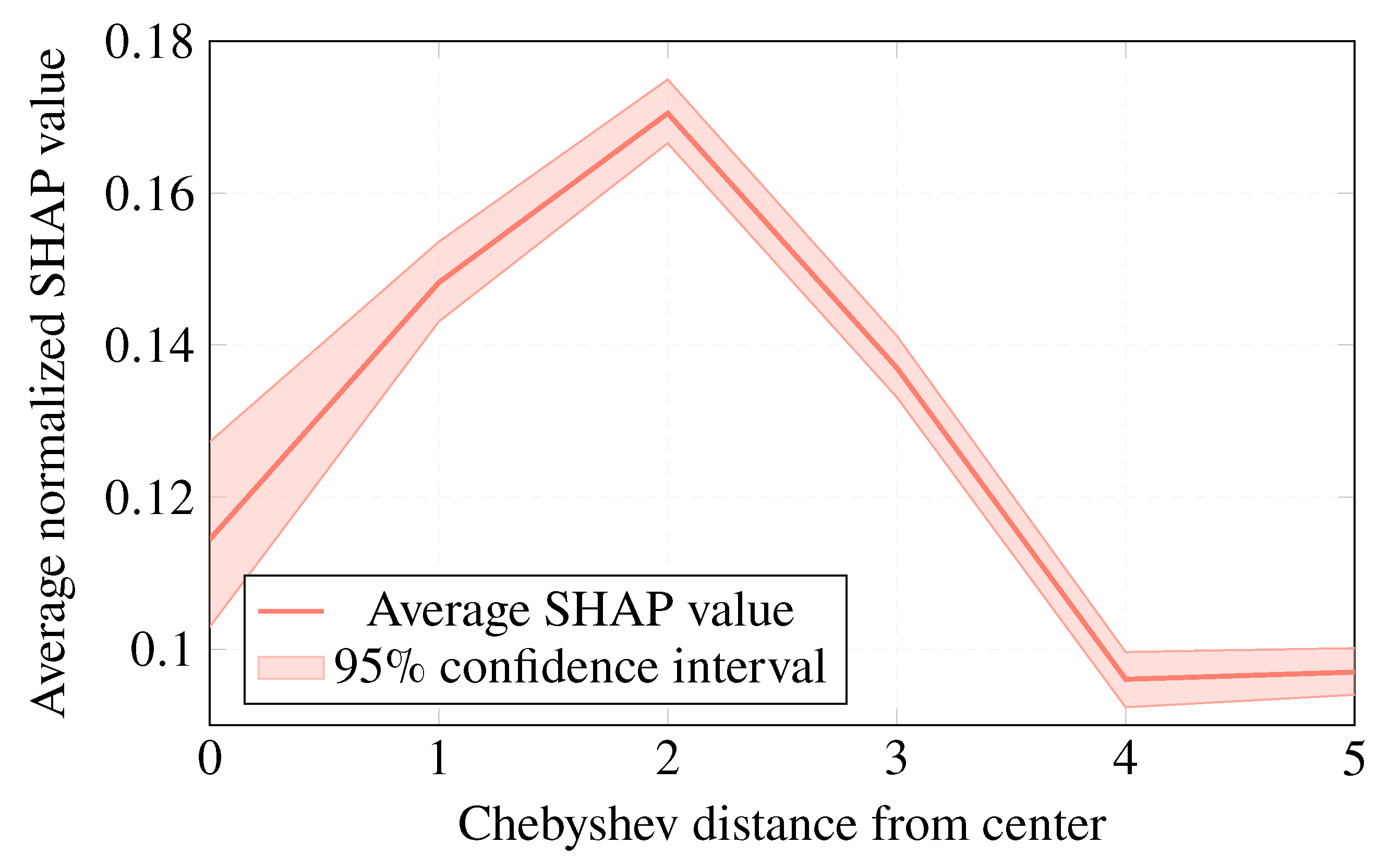
To further interpret SSRs, we examine importance as a function of spatial location. Figure 4 plots average SSR SHAP values versus Chebyshev distance (in SSR-bin units) from the deployment center, using the same normalization as before. Importance peaks around distance two ( 2 r ), indicating that bins located roughly two radii from the center (where devices are better positioned to act as relays between peripheral clusters and the central gateway) are especially informative for gateway placement. Central bins are less informative because centrally located devices are often already in coverage and thus provide less guidance for repositioning gateways.
End-device weights exhibit the lowest marginal SHAP values, yet they remain important when considered collectively. Indeed, weights and CF were the only additional inputs introduced between the first- and second-stage networks in [8], and consistent CF reductions were achieved only after incorporating these blocks.
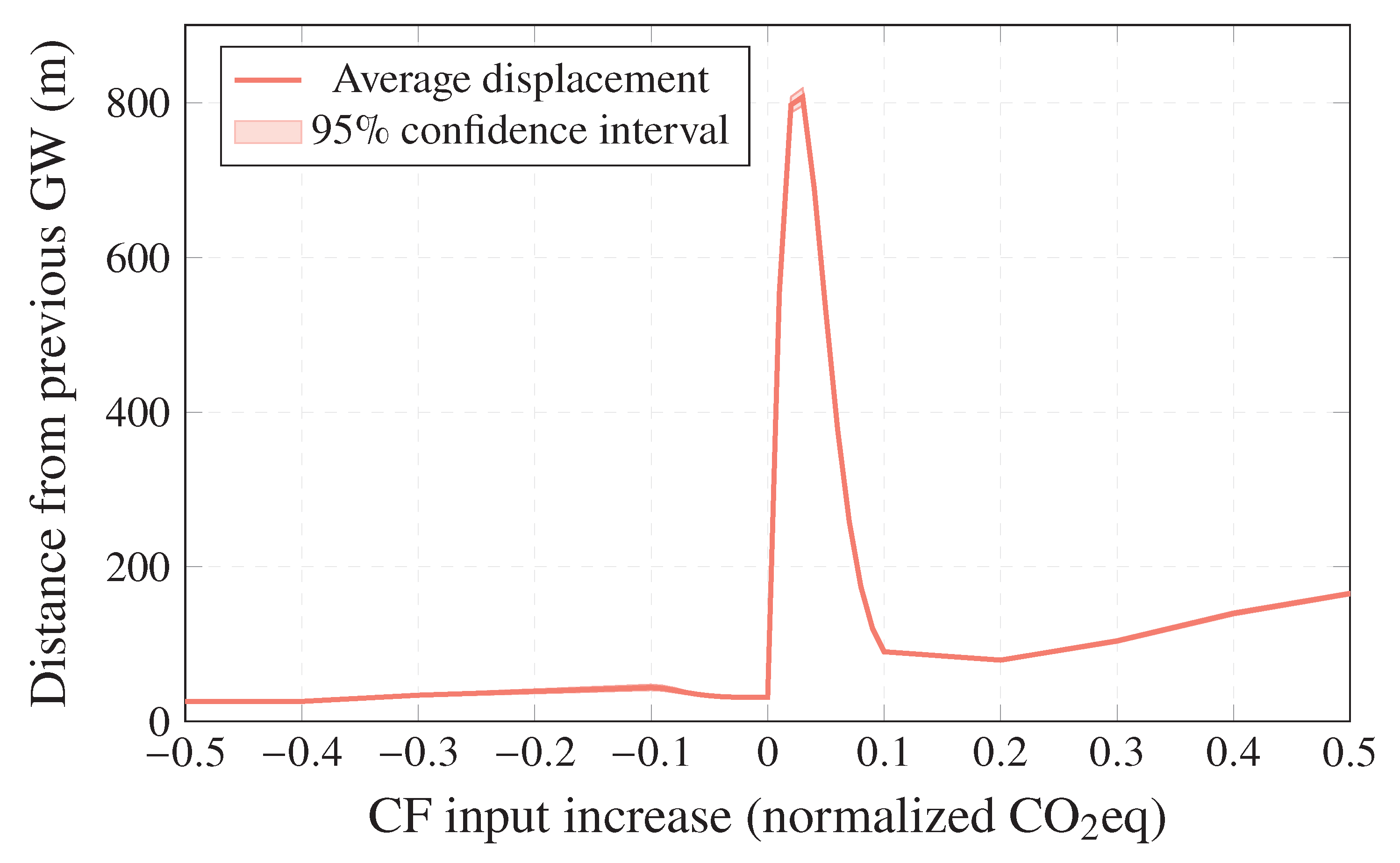
Finally, Figure 5 presents a sensitivity analysis for the normalized CF input. We perturb this value and measure the resulting gateway displacement. CF works as a coarse, global guidance signal: larger CF values trigger larger gateway relocations, with the most pronounced effect occurring for CF increases between 0 and 0.1 in normalized units. It is important to note that this CF is computed from the intermediate network configuration available before the second-stage prediction and is not derived from the ground-truth gateway coordinates used as labels. In this sense, CF summarizes the current environmental inefficiency of the deployment, thereby providing the model with information about the available margin for improvement. Nevertheless, CF alone does not determine the final placement. The remaining inputs are required to refine the relocation and accurately position the gateway, indicating a clear separation between global decision cues and local spatial adjustment.
The framework used in this paper—combining SHAP, ablation, sensitivity analysis, and weight inspection—can be applied to other supervised learning models, since these tools are either model-agnostic or adaptable to different architectures. However, it is important to distinguish between the transferability of the explainability framework and the transferability of the numerical explanations. The exact numerical attribution values reported here should be considered specific to the trained MLP, the dataset, and the adopted two-stage learning pipeline. As also discussed in recent work on the transferability of local model-agnostic explanations [14,21], explanation values obtained for one trained model are not necessarily directly transferable to another model. Consequently, what is expected to generalize is not the precise SHAP value or the exact ranking magnitude of each feature group but the qualitative interpretation of the information roles identified by the combined analyses. In particular, CF-like inputs are expected to remain useful as global descriptors of the intermediate network state and of the available margin for improvement, while coordinates, SSRs, and traffic weights provide complementary local spatial and relay-related information.

4. Discussion

This work investigated which input information is most relevant for an MLP-based gateway placement pipeline designed to minimize the carbon footprint of LoRa-based multi-hop networks. Building on our previous studies, which introduced the CF model, the ILP formulation, and the learning-based approximation of the optimal gateway position [7,8], the present manuscript shifts the focus from optimization performance to model understanding. The objective is not to propose a new neural architecture but to determine which input features should be retained, combined, or interpreted with caution when designing future CF-aware learning pipelines. In this sense, the explainability analysis leads to three concrete input-design recommendations for green communications design.
First, providing an accurate CF estimate for the current network state is indispensable. The CF scalar acts as a high-level guidance signal that tells the model when substantial reconfiguration is warranted; small changes in the CF input can produce large gateway relocations. Because the CF drives both the objective and the model’s coarse decisions, accurate life-cycle and operational-emission modeling is essential for any CF-aware planning pipeline.
Second, representing end-device positions using both raw coordinates and SSRs yields the best empirical performance, despite the redundancy. Coordinates supply fine-grained location cues necessary for precise placement, while SSRs provide a robust, fixed-length spatial summary that highlights locality-structured phenomena. SSRs are particularly effective at surfacing collective relay opportunities; although each SSR bin has small marginal influence, their combined signal is essential for good CF-aware decisions.
Third, end-device weights (the log-transformed transmitted traffic) convey information that resembles the “force” concept introduced in [6]: both quantify the relative influence of end devices as potential traffic relays. We find that weights help contextualize raw coordinates by highlighting which end devices are more influential, but on a per-feature basis, they consistently show the lowest marginal importance among the inputs we evaluated. Their main value therefore lies in collective effects: the ensemble of 30 weights helps fine-tune placements even though individual weight entries appear weak in isolation.

Research Limitations and Future Work

These findings point naturally to online and mobile extensions for green communications. An RL agent controlling one or more mobile relays (e.g., drones or mobile gateways as proposed by [3,5]) is a promising next step. Such a policy could learn to place a mobile gateway in real time to reduce the CF under dynamic traffic and energy conditions, leveraging the same spatial and CF-aware encodings studied here. In practice, two important caveats must be considered. (i) A mobile gateway can exploit positions of nearby end devices to quickly optimize local coverage. However, without knowledge of distant devices, full coverage cannot be guaranteed. Relay information from sufficiently connected neighboring devices may provide a useful approximation. (ii) RL agents must be trained and evaluated using the same CF-aware life-cycle accounting used for static planners so that the learned policies truly optimize environmental impact rather than proxy metrics. A hybrid approach combining a fast MLP for coarse gateway suggestion with an RL policy for local refinement remains a promising direction for dynamic deployments.
Future work should also investigate architectures that explicitly incorporate permutation-invariant or graph-based inductive biases. Deep Sets and PointNet-like models could process unordered end-device sets more naturally and support variable network sizes, while graph neural networks (GNNs) could exploit the communication graph defined by feasible links, relay paths, or neighborhood relations. Such models may be particularly useful in larger, denser, or multi-gateway scenarios. Future studies should compare these architectures with the current MLP-based pipeline using the same explainability analyses. This comparison should also re-evaluate the importance of the inputs; this would help determine whether the roles identified in this work for CF, coordinates, traffic weights, and SSRs remain stable across model families. In particular, a systematic multi-architecture study could clarify whether the dominance of CF as a global descriptor and the collective relevance of spatial encodings are properties of the specific MLP used here or more general characteristics of CF-aware gateway placement models.
Although the experiments are conducted on a representative scenario with 30 end devices in a 0.3  km2 urban area, qualitative conclusions are expected to extend beyond that exact setting. What is expected to generalize is not the precise numerical ranking of each feature group, which may vary with deployment density, propagation conditions, and model capacity, but the functional role played by each type of information. In particular, global descriptors such as CF are expected to remain useful for coarse decision guidance, whereas raw coordinates and spatial summaries such as SSRs provide the local geometric information required for precise placement. For larger or denser deployments, the network can be partitioned into spatial clusters. The same single-gateway predictor can then be applied independently to each cluster, yielding a simple and scalable multi-gateway solution. In dynamic environments, the same input decomposition can also support periodic re-optimization. It could also be combined with mobile-relay control strategies, provided that the underlying CF accounting remains consistent with the deployment objective. Nevertheless, a complete stability analysis across multiple network sizes remains an important direction for future work. Such an analysis would require generating additional ILP-labeled datasets for larger deployments. This is computationally demanding because the numbers of end devices, candidate gateway locations, feasible links, decision variables, and constraints grow rapidly with network size.
Several additional limitations should also be considered when extrapolating these results. First, the life-cycle CF model assumes a constant number of end devices and therefore does not optimize the manufacturing or end-of-life emissions of the end devices. As a result, the reported CF reductions should be interpreted as estimates under fixed-device and fixed-lifetime assumptions; in real deployments, additional wear-and-tear costs could reduce or shift the estimated benefit of some configurations, especially those that concentrate forwarding traffic on a small subset of relay nodes. Second, although the discussion points toward real-time, mobile, and drone-assisted extensions, the empirical validation in this work is restricted to static topologies with fixed end-device positions. The framework can also be interpreted as a CF-aware gateway-placement recommendation for a given network snapshot. Therefore, the results demonstrate the suitability of the proposed input representations for static carbon-aware planning, while dynamic operation remains a future research direction that would require time-varying data, mobility-aware constraints, and online validation. Third, the network model assumes pre-programmed next-hop paths and neglects packet collisions and retransmissions. These effects can become relevant in dense or large-scale urban and industrial deployments, particularly as hop count and relay traffic increase. Incorporating a dynamic routing protocol and retransmission-induced energy consumption would likely increase the estimated CF of heavily loaded relay paths and could modify the preferred gateway placement. Network convergence time, defined as the time required for all devices to update their routing tables, would also be relevant in fast-changing environments. Consequently, future work should integrate more detailed medium-access, synchronization, and reliability models to assess the robustness of the learned placement decisions under realistic channel impairments. Finally, the current dataset assumes uniformly random end-device placement and homogeneous traffic. Heterogeneous traffic would alter relay loads, duty-cycle feasibility, and the traffic-based weight feature. While random independent placement produces many spatial configurations, deliberately structured or extreme non-uniform deployments, such as dense hotspots or a concentration of devices at the boundaries, may lead to underperformance if they are not represented during training.

Author Contributions

Conceptualization, F.-J.A.-A. and R.A.-C.; Methodology, F.-J.A.-A.; Software, F.-J.A.-A.; Validation, R.A.-C. and A.-J.G.-S.; Formal Analysis, J.G.-H.; Resources, R.A.-C.; Writing—Original Draft Preparation, F.-J.A.-A.; Writing—Review and Editing, J.G.-H. and A.-J.G.-S.; Visualization, F.-J.A.-A. and R.A.-C.; Supervision, J.G.-H.; Project Administration, J.G.-H.; Funding Acquisition, A.-J.G.-S. All authors have read and agreed to the published version of the manuscript.

Funding

This work was supported by the grant PID2023-148214OB-C21, funded by MICIU/AEI/10.13039/501100011033 and by FEDER/the EU. This work was also supported by the grants PCI2024-153485 and PDC2025-165710-C22, funded by MICIU/AEI/10.13039/501100011033 and by the European Union. Additionally, this research was funded by the PRIMA Programme under Grant Agreement No. 2431 (FUSION: Comprehensive and sustainable solution to minimize food loss and waste and promote food security in the Mediterranean region). The work of Francisco-Jose Alvarado-Alcon was supported by Spain’s Ministry of Universities under Grant FPU22/00316.

Data Availability Statement

No new datasets were created in this study. The raw data supporting the conclusions of this article will be made available by the authors upon reasonable request.

Conflicts of Interest

The authors declare no conflicts of interest.

Abbreviations

The following abbreviations are used in this manuscript:
AIArtificial Intelligence
CFCarbon Footprint
CIConfidence Interval
CSSChirp Spread Spectrum
GNNGraph Neural Network
ILPInteger Linear Programming
IoTInternet of Things
LPWANLow-Power Wide-Area Network
LTELong-Term Evolution
MLPMultilayer Perceptron
MSEMean Squared Error
NNNeural Network
PHYPhysical
RLReinforcement Learning
SDStandard Deviation
SFSpreading Factor
SHAPShapley Additive Explanations
SSRSpatial Sampling Region
XAIExplainable Artificial Intelligence

References

  1. Almuhaya, M.A.; Jabbar, W.A.; Sulaiman, N.; Abdulmalek, S. A survey on Lorawan technology: Recent trends, opportunities, simulation tools and future directions. Electronics 2022, 11, 164. [Google Scholar] [CrossRef] [Scilit]
  2. Marenco, J.; Micheletto, M.; Santos, R. Clustering nodes in Internet of Things environments with time and energy constraints: A multiobjective optimization formulation for the gateway placement problem in LoRaWAN® networks. Int. Trans. Oper. Res. 2025. [Google Scholar] [CrossRef] [Scilit]
  3. Dridi, A.; Laroui, M.; Boucetta, C.; Afifi, H.; Moungla, H. Reinforcement Learning Vs ILP Optimization in IoT support of Drone assisted Cellular Networks. In Proceedings of the ICC 2022—IEEE International Conference on Communications, Seoul, Republic of Korea, 16–20 May 2022; pp. 4589–4594. [Google Scholar] [CrossRef] [Scilit]
  4. Maddikunta, P.K.R.; Gadekallu, T.R.; Kaluri, R.; Srivastava, G.; Parizi, R.M.; Khan, M.S. Green communication in IoT networks using a hybrid optimization algorithm. Comput. Commun. 2020, 159, 97–107. [Google Scholar] [CrossRef] [Scilit]
  5. Tang, W.; Zhao, H.; Chen, S.; Li, A.; Yang, W.; Cheng, W.; Li, Y.; Dong, L. Measurement of LoRa signal propagation in urban areas utilizing aerial gateway and ground gateway. Sci. Data 2025, 12, 1464. [Google Scholar] [CrossRef] [Scilit] [PubMed]
  6. Turlykozhayeva, D.; Waldemar, W.; Akhmetali, A.; Ussipov, N.; Temesheva, S.; Akhtanov, S. Single Gateway Placement in Wireless Mesh Networks. Phys. Sci. Technol. 2024, 11. [Google Scholar] [CrossRef] [Scilit]
  7. Alvarado-Alcon, F.J.; Asorey-Cacheda, R.; Garcia-Sanchez, A.J.; Garcia-Haro, J. Carbon footprint optimization of a LoRa-based multi-hop Industrial Internet of Things network deployment. Comput. Ind. 2025, 172, 104348. [Google Scholar] [CrossRef] [Scilit]
  8. Alvarado-Alcon, F.J.; Asorey-Cacheda, R.; Garcia-Sanchez, A.J.; Garcia-Haro, J. Minimizing the Carbon Footprint in LoRa-Based IoT Networks: A Machine Learning Perspective on Gateway Positioning. IEEE Open J. Comput. Soc. 2025, 6, 531–542. [Google Scholar] [CrossRef] [Scilit]
  9. Alvarado-Alcon, F.J.; Asorey-Cacheda, R.; Garcia-Haro, J.; Garcia-Sanchez, A.J. Carbon Footprint-Aware Gateway Placement in LoRa Multi-Hop Networks: An Input Importance Analysis for Green Communications. In Proceedings of the 2026 EuCNC & 6G Summit, Málaga, Spain, 2–5 June 2026; Extended Abstract Presented as a Two-Page Poster; IEEE: Piscataway, NJ, USA, 2026. [Google Scholar]
  10. Guo, W. Explainable Artificial Intelligence for 6G: Improving Trust between Human and Machine. IEEE Commun. Mag. 2020, 58, 39–45. [Google Scholar] [CrossRef] [Scilit]
  11. Ayoub, O.; Di Cicco, N.; Ezzeddine, F.; Bruschetta, F.; Rubino, R.; Nardecchia, M.; Milano, M.; Musumeci, F.; Passera, C.; Tornatore, M. Explainable Artificial Intelligence in communication networks: A use case for failure identification in microwave networks. Comput. Netw. 2022, 219, 109466. [Google Scholar] [CrossRef] [Scilit]
  12. Roscher, R.; Bohn, B.; Duarte, M.F.; Garcke, J. Explainable Machine Learning for Scientific Insights and Discoveries. IEEE Access 2020, 8, 42200–42216. [Google Scholar] [CrossRef] [Scilit]
  13. Belle, V.; Papantonis, I. Principles and Practice of Explainable Machine Learning. Front. Big Data 2021, 4, 688969. [Google Scholar] [CrossRef] [Scilit] [PubMed]
  14. López González, A.M.; García-Cuesta, E. On the transferability of local model-agnostic explanations of machine learning models to unseen data. In Proceedings of the 2024 IEEE International Conference on Evolving and Adaptive Intelligent Systems (EAIS), Madrid, Spain, 23–24 May 2024; pp. 1–10. [Google Scholar] [CrossRef] [Scilit]
  15. Semtech Corporation. LoRa® and LoRaWAN®. 2024. Available online: https://www.semtech.com/uploads/technology/LoRa/lora-and-lorawan.pdf (accessed on 17 April 2026).
  16. Sherazi, H.H.R.; Piro, G.; Grieco, L.A.; Boggia, G. When renewable energy meets LoRa: A feasibility analysis on cable-less deployments. IEEE Internet Things J. 2018, 5, 5097–5108. [Google Scholar] [CrossRef] [Scilit]
  17. Gaspar, D.; Silva, P.; Silva, C. Explainable AI for Intrusion Detection Systems: LIME and SHAP Applicability on Multi-Layer Perceptron. IEEE Access 2024, 12, 30164–30175. [Google Scholar] [CrossRef] [Scilit]
  18. Lundberg, S.M.; Lee, S.I. A Unified Approach to Interpreting Model Predictions. In Proceedings of the Advances in Neural Information Processing Systems 30, Long Beach, CA, USA, 4–9 December 2017; Guyon, I., Luxburg, U.V., Bengio, S., Wallach, H., Fergus, R., Vishwanathan, S., Garnett, R., Eds.; Curran Associates, Inc.: Red Hook, NY, USA, 2017. [Google Scholar]
  19. Beade, Á.; Rodríguez, M.; Santos, J. Evolutionary feature selection approaches for insolvency business prediction with genetic programming. Nat. Comput. 2023, 22, 705–722. [Google Scholar] [CrossRef] [Scilit]
  20. Charles, R.Q.; Su, H.; Kaichun, M.; Guibas, L.J. PointNet: Deep Learning on Point Sets for 3D Classification and Segmentation. In Proceedings of the 2017 IEEE Conference on Computer Vision and Pattern Recognition (CVPR), Honolulu, HI, USA, 21–26 July 2017; pp. 77–85. [Google Scholar] [CrossRef] [Scilit]
  21. Salih, A.M.; Raisi-Estabragh, Z.; Galazzo, I.B.; Radeva, P.; Petersen, S.E.; Lekadir, K.; Menegaz, G. A Perspective on Explainable Artificial Intelligence Methods: SHAP and LIME. Adv. Intell. Syst. 2025, 7, 2400304. [Google Scholar] [CrossRef] [Scilit]
Figure 1. Topology designed after using our proposed methodology for optimizing the carbon footprint (CF) of LoRa multi-hop networks. Link colors represent the level of link usage, whereas end-device colors indicate the spreading factor (SF) used for transmission. This particular network instance does not include any end device using SF 12; nevertheless, SF 12 is kept in the legend to represent the full range of possible SFs.
Futureinternet 18 00389 g001
Figure 2. Analysis of the weights between the input parameters of the end devices and the nodes of the hidden layer for inputs where (a) symmetry between all inputs is expected or (b) inputs are permutation-sensitive. The maximum length of the whiskers is 1.5 the interquartile range; observations beyond the whiskers are represented by an × symbol.
Futureinternet 18 00389 g002
Figure 3. Normalized Shapley additive explanations (SHAP) values averaged by input category. The 95% confidence interval (CI) has been drawn on top of the bars.
Futureinternet 18 00389 g003
Figure 4. Average SSR SHAP value as a function of Chebyshev distance from the center.
Futureinternet 18 00389 g004
Figure 5. Sensitivity to the CF input: normalized CF is perturbed, and the average resulting gateway displacement is plotted, with the values limited so that the gateway coordinates remain within the network area.
Futureinternet 18 00389 g005
Table 1. Problem parameters and decision variables.
ParameterDescription
α Upper bound on the traffic load that can be assigned to one gateway; in our case, a very large number, α 1 .
C T The total CF of the network in CO 2eq/year.
G k Optimization variable representing whether point k from the grid contains a gateway.
L i , k Optimization variable representing whether a link between end device i and point k exists and the number of traffic units it carries.
L N i , j Optimization variable representing whether a link between end devices i and j exists and the number of traffic units it carries.
N Set of end devices in the network.
nNumber of end devices in the network, n = | N | .
P Set of candidate gateway locations in the network.
pNumber of points where a gateway could be placed in the network, p = | P | .
P T x i , k Fraction of time end device i must transmit to send one unit of traffic to point k.
P T N x i , j Fraction of time end device i must transmit to send one unit of traffic to end device j.
Table 2. Neural network test subset inputs and their corresponding quantities: end device coordinates, traffic-based weights, spatial sampling regions (SSRs), and CF. The normalized values are summarized by their mean ± standard deviation (SD) and their median.
Input Type#RangeNormalizedMean ± SDMedian
Coordinates60[0, 547.7][0, 1]0.5 ± 0.290.5
Weights30[log(1), log(30)][0, 1]0.21 ± 0.240.20
SSRs121[0, 7][0, 0.88]0.09 ± 0.110.12
CF1[11.12, 44.48][0, 0.38]0.02 ± 0.070
Table 3. Pairwise comparison of the mean absolute normalized SHAP values of CF against the remaining features. Mean differences are computed as CF feature .
ComparisonMean Differencep-Valuet-StatisticBootstrap 95% CI
CF–Coordinates0.14760.00172.94[0.0551, 0.2503]
CF–Weights0.4360<0.00018.90[0.3455, 0.5380]
CF–SSRs0.3706<0.00017.69[0.2844, 0.4676]
Disclaimer/Publisher’s Note: The statements, opinions and data contained in all publications are solely those of the individual author(s) and contributor(s) and not of MDPI and/or the editor(s). MDPI and/or the editor(s) disclaim responsibility for any injury to people or property resulting from any ideas, methods, instructions or products referred to in the content.