A Hybrid CNN–LSTM Model for IoT Intrusion Detection: A Robustness Analysis Across Datasets

Abstract

The rapid growth of Internet of Things (IoT) devices has led to security concerns due to increasing IoT attacks. Traditional intrusion detection systems (IDS) struggle to effectively detect attacks due to the evolving nature of threats and heterogeneous traffic patterns. Therefore, this study presents a structured and reproducible intrusion detection approach that integrates preprocessing and deep learning-based classification for binary detection in IoT networks. The datasets used are ToN_IoT and UNSW-NB15 datasets, which contain IoT network traffic data. This study deploys a meta-heuristic algorithm called Gray Wolf Optimizer (GWO) for feature selection. SMOTE is used for balancing the class sample, and MinMax and standard normalization for data scaling during preprocessing. A comparative analysis is performed across multiple deep learning models, including Convolutional Neural Network–Long Short-Term Memory (CNN–LSTM), Multi-Layer Perceptron (MLP), Deep Neural Network (DNN), Convolutional Neural Network (CNN), and Recurrent Neural Network (RNN). Results show that the CNN–LSTM model demonstrates strong performance consistency across datasets, achieving 99.68% and 92.05% accuracy on ToN_IoT and UNSW-NB15, respectively. Threshold sensitivity analysis reveals key detection and false-positive trade-offs for edge IDS. Through extensive performance evaluation and sensitivity analysis, this study highlights the importance of combining preprocessing, model evaluation, and threshold analysis for reliable IoT intrusion detection.

1. Introduction

The exponential growth of Internet of Things (IoT) deployments has fundamentally transformed network security landscapes by introducing billions of heterogeneous devices, which include resource-constrained devices across smart homes, industrial control systems, healthcare monitoring, and critical infrastructure. As of 2026, there are more than 35 billion IoT devices worldwide, and the attack surface for these devices is becoming very large, thereby making conventional security measures insufficient [1,2,3]. In reality, IoT traffic is generated and locally processed at distributed endpoints and gateways; hence, centralized heavyweight security monitoring can be infeasible (due to cost and operational overhead).

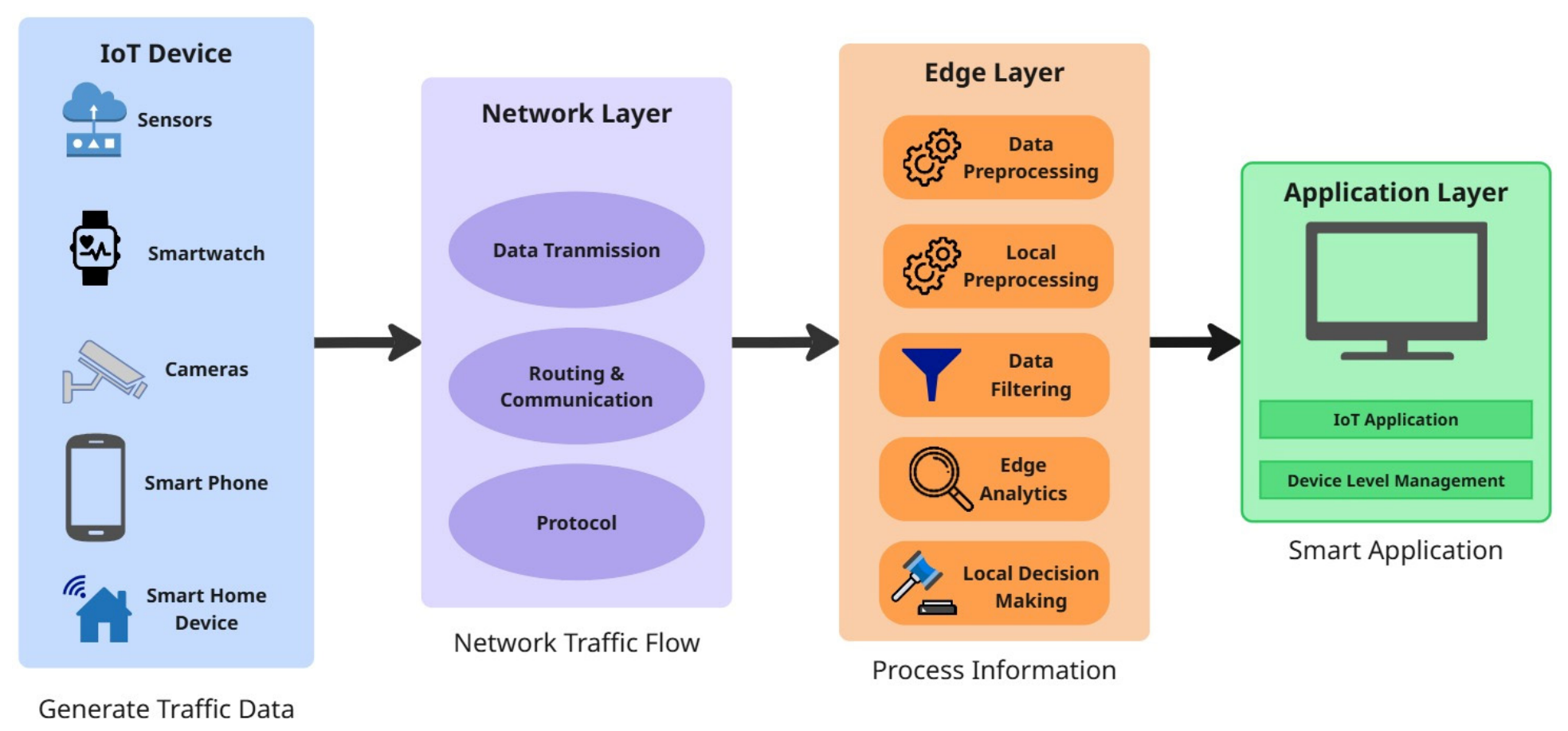
Figure 1 describes the architecture of the proposed IoT-based Intrusion Detection System (IDS). The architecture of the proposed IoT-based IDS comprises four layers, namely, the IoT device layer, the network layer, the edge layer, and the application layer. The IoT layer comprises heterogeneous devices such as sensors, cameras, and smart home devices that generate network traffic data. The network layer is responsible for facilitating the transmission of data, its routing, and communication between the IoT devices and the edge layer via communication protocols. The edge layer is essential in the operation of the IoT network as it acts as the link between the IoT layer and the application layer [4]. This is where processing, filtering, and analysis of data collected by IoT devices take place. This can be achieved by using gateway devices. The proposed intrusion detection model is deployed within this layer to analyze network traffic and identify potential security threats. The application layer facilitates security monitoring, visualization, and alerts based on the results of intrusion detection.

In this study, it also focuses on IoT networks that exhibit unique security threats complicating intrusion detection. First, many IoT devices have very constrained processing power, memory, and energy resources, which can preclude resource-intensive security mechanisms at the device level [5]. Second, IoT traffic is naturally heterogeneous. While sensor telemetry, actuator commands, and control messages are legitimate types of communication, the exchanged information is affected by different types of attacks, such as volumetric Denial-of-Service (DoS) floods on one side and discrete reconnaissance or exploitation attempts on the other [6]. Third, IoT environments frequently change by means of device inclusions, exclusions, and firmware updates, and attacker strategies evolve, which requires the use of adaptive detection techniques that are not dependent on static signatures [7]. These characteristics render traditional signature-based IDS inadequate in detecting zero-day attacks and in generating a high false-positive rate (FPR) when facing varying IoT traffic patterns [8]. Even anomaly-based approaches struggle due to the challenging to create baseline of “normal” behavior in settings where benign behavior evolves over time [9]. These limitations motivate the adoption of machine learning and deep learning techniques that can learn complex patterns from high-dimensional network data and support more adaptive intrusion detection.

While deep learning has achieved state-of-the-art performance in multiple security domains [10,11], applying it directly to IoT intrusion detection introduces challenges that require careful architectural design. A key issue is temporal dependency, which real attack campaigns frequently unfold over multiple time steps, progressing from reconnaissance to exploitation, meaning that temporal context can be essential for separating benign periodic transmissions from malicious sequences [12]. However, feedforward models such as Multi-Layer Perceptron (MLP) and Deep Neural Network (DNN) typically process flows independently, which can discard the sequential patterns needed to detect multi-stage attacks where individual events appear benign in isolation.

Another difficulty is exploiting the local correlation in network features. Network traffic characteristics frequently have structured correlations, such as correlations among packet sizes, protocol behaviors, port usage, and service patterns that a Convolutional Neural Network (CNN) can learn effectively through local filters [13]. Nevertheless, CNNs lack inherent mechanisms for modeling longer sequential dependencies, which limits their ability to represent how attack behaviors evolve. Finally, IoT deployments impose strict resource–performance constraints, especially at edge gateways that must operate under limited memory and compute budgets. Although deep models may be expensive to train, they can be optimized for deployment through techniques such as pruning and quantization, enabling efficient inference compared with complex ensemble approaches that may require excessive memory and computation [14]. These considerations motivate hybrid architectures, such as CNN–LSTM, that can balance spatial feature extraction with temporal modeling while remaining feasible for edge deployment.

Despite the increasing number of CNN–LSTM research works in the domain of network intrusion detection [15,16,17], a few challenges affect its practical application and scientific comparison. First, several studies rely heavily on evaluating models using only single-point metrics such as accuracy and F1-score, without considering full Receiving Operating Characteristic (ROC) analysis and threshold sensitivity, which are crucial in real-world scenarios where detection rate vs. false positives trade-offs need to be taken into account [18]. Secondly, evaluation is based on just one dataset, hence providing limited insights into how models behave in the case of differences in data distributions. Evaluation of performance variability across several datasets is crucial for analyzing the robustness of the intrusion detection models when applied to real-world IoT environments [19]. Third, preprocessing pipelines, including feature selection, data balancing, and feature scaling, are often under-specified, despite their significant impact on model performance, computational efficiency, and reproducibility, particularly in high-dimensional and imbalanced datasets [20]. This limitation makes it difficult to compare models fairly and reduces the effectiveness of IDS implementation in IoT settings.

To address these issues, this study makes four main contributions. First proposes a structured and reproducible intrusion detection approach that integrates preprocessing and learning components into a unified pipeline, including Gray Wolf Optimizer (GWO)-based feature selection for reducing the number of features to 30, Synthetic Minority Over-sampling Technique (SMOTE) for class balancing, and feature scaling (from MinMax to standardization) for improving the feature quality, enhancing class separation, and lowering the complexity of computations. Second, it conducts a robustness analysis across datasets using the ToN_IoT and UNSW-NB15 benchmarks, where performance variation is quantified through ΔAccuracy and ΔReceiver Operating Characteristic–Area Under the Curve (ROC-AUC) to provide insight into model behavior under differing data characteristics. Third, it presents a threshold-aware evaluation based on ROC curves and sensitivity analysis to support deployment-oriented decision-making, enabling the selection of operating points that balance detection performance and false-positive rates according to organizational requirements. Finally, it features a hybrid CNN–LSTM model that leverages convolutional networks to extract relationships between spatial feature characteristics while making use of Long Short-Term Memory (LSTM) for temporal dependency modeling. The focus is not on proposing a new architecture, but on demonstrating how model performance is influenced by integrated preprocessing and evaluation strategies in realistic intrusion detection settings.

The remainder of this paper is organized as follows. Section 2 describes the methodology, including the datasets, preprocessing pipeline, model architectures, and evaluation protocols. Section 3 presents the results and discussion, covering ROC analysis, cross-dataset performance, and deployment implications. Section 4 concludes with the key findings, limitations, and directions for future research.

2. Related Work

Numerous studies have explored hybrid deep learning architectures such as CNN–LSTM for intrusion detection in IoT environments, often evaluated on datasets such as UNSW-NB15 and ToN_IoT. While these approaches demonstrate strong detection performance, many focus primarily on architectural design without systematically integrating feature selection, data balancing, or threshold-aware evaluation. Furthermore, limited attention has been given to cross-dataset robustness and the impact of preprocessing on model performance.

As illustrated in

Table 1. Comparison of recent IoT intrusion detection approaches and their limitations.

Study	Model	Dataset	Key Method	Limitation
[21]	CNN, LSTM	ToN_IoT	Deep learning	Does not employ wrapper-based feature selection, limiting feature optimization
[22]	LSTM	UNSW-NB15	Sequential modeling	Does not address class imbalance, leading to potential bias in detection
[23]	Hybrid (CNN–LSTM)	ToN_IoT	Hybrid deep learning	Lacks threshold-aware evaluation, limiting decision adaptability
This work	CNN–LSTM + GWO	ToN_IoT & UNSW-NB15	Feature selection + SMOTE + ROC-based threshold analysis	-

, the current literature concentrates more on the architecture of the model, like CNN, LSTM, or even both CNN and LSTM, with testing conducted on one dataset alone. Many studies also do not utilize wrapper feature selection methods, do not solve class imbalance problems, or do not consider threshold-based evaluation, which could be a hindrance to the efficacy and adaptability of the models developed. In contrast, the proposed approach integrates GWO for feature selection, SMOTE for balancing, scaling, and even threshold-based evaluation using the ROC method. The study further evaluates the robustness of the model across two different benchmark datasets.

3. Materials and Methods

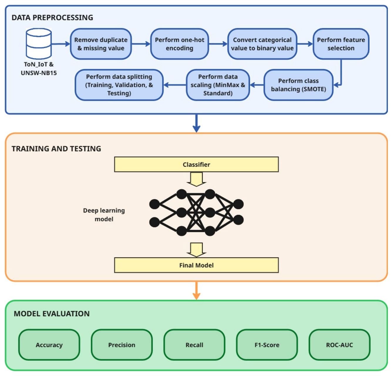
The following section presents the methodology used in this study for IoT intrusion detection. It describes the datasets, data preprocessing, feature selection pipeline, the proposed CNN–LSTM model, baseline methods, and the ROC-based evaluation. Each step is included to support reproducibility and to demonstrate the effectiveness of the proposed model. Figure 2 shows the overall flow of the study’s methodology.

The experiments were conducted using Google Colab with a CPU runtime environment. The local computer used to access the platform had the following specifications: an Intel i5 processor, 16 GB of RAM, and an NVIDIA GeForce RTX 4050 GPU with 6 GB memory. The operating system was Windows 11. The implementation was executed using Python 3.12.13 with the following software packages: NumPy 2.0.2, Pandas 2.2.2, Matplotlib 3.10.0, PyTorch 2.11.0+cpu, Scikit-learn 1.6.1 for implementing traditional machine learning models, and Imbalanced-learn 0.14.1 for data balancing.

3.1. Dataset

This study evaluates the proposed CNN–LSTM architecture and baseline methods using the ToN_IoT and UNSW-NB15 benchmarks, which represent complementary threat landscapes and network characteristics.

The ToN_IoT dataset [24] provides comprehensive network and telemetry data from heterogeneous IoT devices, including smart home appliances, industrial sensors, and edge gateways. Generated in a controlled testbed environment at UNSW Canberra using NSX vCloud NFV platform, the dataset captures realistic attack scenarios against diverse IoT platforms running Linux, Windows, and embedded operating systems. The dataset used is the network dataset, which was collected in the Comma-Separated Values (CSV) files. The dataset contains 211,043 samples with 44 features spanning packet-level statistics, protocol metadata, and system telemetry. This dataset has multiple categories related to the attacks, such as DoS, Distributed Denial of Service (DDoS), backdoor infiltration, command injection, and scanning-based reconnaissance. The class distribution of binary classes is imbalanced, with 50,000 normal and 161,043 attack samples. Temporal patterns present in connection duration, spatial relationships observed in packet size distribution, and protocol-level features such as Transmission Control Protocol (TCP) flag combinations and service port usage are among the aspects that these features recognize about network behavior. ToN_IoT is a novel dataset that combines network flow data with IoT and Industrial Internet of Things (IIoT) telemetry gathered from seven services used in real life, including weather sensors, smart garage controllers, refrigerators, Modbus industrial protocols, Global Positioning System (GPS) trackers, motion-activated lighting, and thermostats via Message Queuing Telemetry Transport (MQTT) messaging. This multi-modal structure accounts for realistic heterogeneity and introduces unique challenges with respect to model adaptability across different types of data. The combined scenarios present a realistic representation of IoT use cases, where edge gateways will have to deal with the traffic produced by all types of devices and their specific communication behaviors.

The UNSW-NB15 dataset [25] captures modern network attack behaviors through synthetic traffic generated by the IXIA PerfectStorm tool under contemporary threat models. This is a synthetic dataset developed by the Cyber Range Lab at the Australian Centre for Cyber Security, which extracts 257,673 records described by 45 features from packet captures with Argus and Bro tools. Unlike ToN_IoT, which comprises traffic specific to the IoT domain, UNSW-NB15 focuses on network-layer attacks across an array of nine attack families, such as exploits, fuzzers, reconnaissance, shellcode, and worms. The dataset is used for binary classification to differentiate between normal traffic (93,000 samples) and all types of aggregated attack traffic (164,673 samples), including fuzzers, analysis activity, backdoors, DoS attacks, exploits, generic attacks, reconnaissance attempts, shellcode injections, and worms. The set of features includes network flow characteristics like their inter-arrival timings and byte sizes, protocol features such as TCP window size distributions and flag patterns, as well as temporal aggregations covering data transfer duration or rates. The network-centric perspective of this dataset complements the device-centric view in ToN_IoT and allows for assessment of model robustness across different threat focuses and traffic characteristics.

Table 2. The information on datasets.

Dataset	Label	Number of Samples	Number of Features
ToN_IoT	Benign	50,000	44
	Attack	161,043
UNSW-NB15	Benign	93,000	45
	Attack	164,673

presents a summary of the datasets.

Table 2 summarizes the two datasets used in this study, including their class labels, sample counts, and the number of features, evaluating performance using both ToN_IoT and UNSW-NB15 in different traffic characteristics and threat models. With telemetry comprising heterogeneous devices, the ToN_IoT dataset enables the assessment of model performance under IoT-specific common patterns like messaging in MQTT, industrial protocols, or streaming sensor data. By contrast, UNSW-NB15 was developed specifically for network-layer attacks to evaluate model robustness in traditional network security scenarios, leveraging packet-level features and protocol-based characteristics. Testing the CNN–LSTM model with these datasets separately will provide insight into whether the model learns robust and transferable intrusion patterns across different environments, or whether it primarily captures dataset-specific statistical properties that limit its effectiveness under varying traffic conditions. The discrepancy between performance on the datasets gives insight into the divergence between a controlled benchmark setting and an actual deployed environment, where traffic distributions will naturally differ.

3.2. Data Preprocessing Pipeline

The preprocessing pipeline includes a total of four sequential stages that help to tackle issues regarding high dimensionality, class imbalance, and feature scaling-specific properties related to network intrusion data. It consists of several steps that have different goals while maintaining data integrity by preventing loss between the testing and training parts of the data.

The first step in pre-processing is removing duplicate and missing value data, and one-hot encoding for categorical variables. For the ToN_IoT dataset, categorical protocol variables such as TCP, User Datagram Protocol (UDP), Internet Control Message Protocol (ICMP), and Application-layer service types are encoded as binary indicator variables. The same is done for protocol state variables and connection flags. Binary or Boolean values are assigned to coded features from UNSW-NB15, such as protocol, service identifiers, or connection state variables.

The label variable will be changed from a string type to a binary type, where 0 represents normal traffic and 1 represents attack traffic for both datasets. This binary approach is consistent with the deployment requirements, where the edge IDS must be able to rapidly classify traffic as benign or malicious without necessarily knowing the attack classes in detail. One-hot encoding will be done for categorical variables that have string values. This will increase the feature space of the data. For instance, the feature space of the ToN_IoT dataset will be increased after one-hot coding.

This study employs GWO [26], a nature-inspired metaheuristic algorithm, for wrapper-based feature selection that evaluates feature subsets through actual model performance rather than statistical correlations alone. GWO simulates the leadership hierarchy and hunting mechanism of gray wolf packs through alpha, beta, delta, and omega roles representing solution quality tiers. The algorithm iteratively refines candidate feature subsets by balancing exploration of the search space through global search guided by multiple pack members against exploitation of promising regions through local refinement near best solutions.

Table 3. Gray Wolf Optimization parameter description.

Component	Description
Objective/fitness value	Accuracy
Fitness evaluation split	Train: 80%, Test: 20% (used in feature selection)
Classifier	Random Forest
GWO population	20 wolves
GWO iterations	30 iterations
Forced selected features	30 features

presents the GWO parameters used in this study.

Table 3 presents the configuration of the GWO. The fitness function evaluates the feature subsets using Random Forest classification accuracy using the same train–test split defined in the preprocessing stage (80% training and 20% testing). During this step, the Random Forest algorithm is used to train the training set and evaluate the testing set to obtain the fitness measure. There will be no further internal split carried out in the GWO algorithm. The GWO algorithm is implemented using 20 wolves for 30 generations; each wolf undergoes an update and is then transformed into a binary feature mask of exactly 30 features. The objective function trains a Random Forest model only on the selected features and returns the resulting test accuracy as the fitness score.

It is important to highlight that employing the test partition within the feature selection procedure can create a possible danger of overfitting for the chosen data partitioning scheme. Nevertheless, the ultimate testing of the deep learning models is done independently with the aid of validation and test sets that have not been used for training, allowing us to address the problem effectively.

This dimensionality reduction directly enables edge deployment by minimizing the memory needed to store feature vectors, while decreasing inference latency on the number of operations per prediction and enhancing model interpretability by focusing on features. When the dimensionality and number of features are reduced, there is less risk for overfitting as the hypothesis space becomes constrained, and they will have better robustness to noise due to not including irrelevant or redundant features. The wrapper approach ensures that feature selection provides significant information regarding the target variable rather than just having a statistical relation to the target variable.

3.3. SMOTE Class Balancing

To address class imbalance found in intrusion datasets where normal traffic is predominant, this study implements the SMOTE [27] as SMOTE (random_state = 42), which executes via fit_resample(X, y), yielding the upsampled features with respective labels for model training and evaluation. The present implementation only defines the random seed within the code (all other SMOTE settings, including n_neighbors, are defined as their library default). This is done over line segments joining real attack examples: given each minority sample x, choose one of its k nearest neighbor minority samples x_nn randomly and create a synthetic example as follows: x_new = x + λ(x_nn − x) for random λ ~ Uniform(0, 1).

The synthetic samples are created through convex combinations of existing samples, ensuring that they lie within the same regions of the feature space where real attacks exist; thus, this process augments the training set examples, which allows classifiers to learn decision boundaries that better represent minority class distributions. The application of SMOTE to training data only avoids information leakage that would derive from synthetic generation if test data were influenced by it, an issue that could artificially improve performance metrics. No resampling is performed on the validation and test sets to prevent data leakage and avoid overly optimistic performance estimates. The balanced training set allows models to learn discriminative boundaries without being biased towards the majority class. The importance of prioritizing recall in attack detection is that a false negative can lead to undetected breaches and lateral movement, which are major security concerns for the enterprise security posture [28].

For clarity, it should be noted that the SMOTE algorithm was applied to the minority class regardless of whether the class represented normal traffic or attack traffic. In the ToN_IoT dataset, where attack traffic instances exceeded benign traffic instances, SMOTE was used to up-sample the benign class. Similarly, in the UNSW-NB15 dataset, where attack samples also outnumbered normal samples, SMOTE was applied to up-sample the normal class. This approach ensures that both classes have equal representation during training, allowing the model to learn an unbiased decision boundary irrespective of the varying nature of datasets.

3.4. Dual-Stage Scaling

The two-stage normalization technique employed in this study involves the application of MinMax scaling followed by Standard scaling [29]. In stage 1, feature set MinMax normalization is performed to normalize features into a range of [0, 1] using the formula x_scaled = (x − x_min)/(x_max − x_min), which is intended to mitigate the large scale differences that exist between feature sets with orders of magnitude differences, such as packet transmission rates in the range of [0, 100,000] and normalized timestamp values in the range of [0, 1]. This operation also provides a bound on the gradient calculation, ensuring that large numbers are not dominating backpropagation.

In stage 2, standard scaling (z-score normalization) is done on the MinMax scaled features by setting the mean to zero and the variance to one using x_standardized = (x − μ)/σ. This normalized the parameters into statistically significant info that could be utilized for gradient descent optimization. The sequential application of MinMax and Standard scaling leverages the strengths of both, where MinMax provides the bounded output range that can help clip the influence of outliers during early training stages, while Standard provides faster convergence during later epochs.

The scaling parameters (min, max, mean, and std) are calculated based solely on the training data statistics. The parameters are then applied to transform the validation and test datasets using the same learned transformations, which prevents data leakage where the test data statistics influence the preprocessing.

3.5. Experimental Design

The experimental protocol of this study implements stratified train-validation-test partitioning to preserve a representative distribution of classes in each subset and temporal order whenever relevant for time-series datasets. The split is 80% training set and 20% testing set for both datasets [30]. Stratification maintains attack-to-normal proportions in every split and is key to fair evaluation with class imbalance, because random splitting may randomly generate test sets with different prevalences of class than the train.

The SMOTE balancing on the training partition after having split, leaving the validation and test sets with original class distributions to better resemble a real use case in deployment. This guarantees evaluation metrics reflect the true generalization performance on imbalanced real-world traffic, as opposed to smoothed balanced conditions, which overstate production effectiveness. And this is done without contaminating the test set. The validation set is used to select hyperparameters and determine when to stop training.

All five models are trained on the same preprocessed data to allow a fair comparison. The hyperparameters for each model, including architectural configurations (e.g., number of layers and hidden units), optimization settings (e.g., learning rate and optimizer), and training parameters (e.g., batch size and number of epochs), are predefined based on empirical design choices and commonly adopted settings in prior studies. Specifically, all deep learning models are trained using the Adam optimizer with a learning rate of 0.001.

The validation set is used for evaluating the performance of the model while training and observing its generalization capabilities. Automated hyperparameter tuning techniques like grid search or random search are not used for optimizing the model parameters. The same hyperparameters are used for all the models to ensure consistency in performance results.

The final evaluation metrics are reported using a held-out test set that is not used during model development. This strict separation between training, validation, and testing phases ensures an unbiased assessment of model performance and prevents data leakage.

3.6. Model Architecture

As depicted in Figure 3, the hybrid CNN–LSTM network with convolutional layers (for spatial feature extraction) and recurrent units (for temporal dependency modeling) models structured dependencies within the feature space. The model uses 30 selected features as input, which is reshaped into a tensor of shape (sequence length = 1, features = 30) to enable compatibility with the Conv1D layer. It is important to note that the temporal dimension in this representation does not correspond to true time-series sequences of network flows; rather, it represents a pseudo-sequential arrangement of features within a single sample. In this way, the neural network can detect interrelations between features on a local level without increasing complexity too much, although it may limit the ability to explicitly model multi-step or long-term temporal attack evolution.

Its convolutional stage consists of a Conv1D layer with 32 filters, kernel size 3, Rectified Linear Unit (ReLU) activation, and valid padding that applies learnable filters across the feature dimensions to capture local correlations, such as combinations of traffic-rate indicators and packet-size behaviors that may correspond to scanning or flooding patterns. These resulting representations are then fed into an LSTM layer containing 32 hidden units to learn higher-level dependencies using gating mechanisms that determine which information gets retained, updated, and exposed in the state of the hidden layer. To prevent overfitting, dropout regularization is applied after the LSTM layer with a rate of 0.3 by dropping activations randomly during training to improve model stability and reduce sensitivity to training data variations. A final dense output layer with one neuron and sigmoid activation produces a probability score in the range [0, 1] for binary classification (a hard decision can be made at a default threshold of 0.5; however, ROC analysis assesses performance considering the entire range of thresholds). This approach first captures low-level feature co-occurrence patterns within the convolutional stage and then integrates these representations in the recurrent stage of learning, thus facilitating multi-scale learning, supporting effective intrusion detection. CNN and LSTM architectures have become the top deep learning techniques in IoT network intrusion detection [31,32].

Table 4. Model architecture and training configuration.

Component	CNN–LSTM	DNN	MLP	CNN	RNN
Conv Layers	1 (32 filters, k = 3)	-	-	2 (32, 64 filters, k = 3)	-
LSTM Units	32	-	-	-	-
RNN Units	-	-	-	-	32
Hidden Layers	-	128–64–32	64–32	-	-
Activation	ReLU	ReLU	ReLU	ReLU	-
Output Activation	Sigmoid	Sigmoid	Sigmoid	Sigmoid	Sigmoid
Loss Function	BCEWithLogitsLoss	BCEWithLogitsLoss	BCEWithLogitsLoss	BCEWithLogitsLoss	BCEWithLogitsLoss
Optimizer	Adam	Adam	Adam	Adam	Adam
Learning Rate	0.001	0.001	0.001	0.001	0.001
Batch Size	256	256	256	256	256
Epochs	50	50	50	50	50

presents the model architecture and the training configuration. The hyperparameters used in the designed CNN–LSTM model and baseline models were selected in advance without using any automation techniques. In detail, the CNN–LSTM model has only one convolutional layer with 32 kernels and a kernel size of 3, as well as an LSTM layer with 32 neurons. As baseline models, an MLP with two hidden layers of 64 and 32 neurons, a DNN with three hidden layers of 128, 64, and 32 neurons, a CNN model with two convolutional layers (filters 32 and 64), and a simple RNN with 32 neurons have been used.

All models were trained with the Adam optimizer using a learning rate of 0.001 for 50 epochs and a batch size of 256. ReLU activation was used for hidden layers, while the activation in the output layer was based on the sigmoid activation function. Training of the models was done using binary cross-entropy loss with logits. Validation data was used to keep track of the model’s performance during training, while testing data was used for the evaluation of the model’s performance after training. No hyperparameter tuning techniques, such as grid search and random search, were used in the process of training the models.

3.7. Training Configuration

All models are trained with a binary cross-entropy loss function L = −[y log(ŷ) + (1 − y) log(1 − ŷ)] where y is the true label and ŷ is the predicted probability. Loss function that penalizes confident predictions more than uncertain ones, gives stronger gradient signals for learning more robust decision boundaries. It employs Adam optimizer with default parameters and an initial learning rate of 0.001, which adjusts the individual learning rates for each parameter through momentum and the RMSProp-like scaling. Adam’s adaptive learning rates also speed up convergence over vanilla stochastic gradient descent, while keeping training stable.

Training runs up to 50 epochs with early stopping on validation loss to avoid overfitting. Early stopping stops training if the validation loss does not improve after 10 epochs (patience = 10) and restores weights from the epoch with the minimum validation loss. This regularization strategy avoids overtraining, when models start memorizing training data instead of learning meaningful feature representations. With a batch size of 128, there is a balance between the memory efficiency of the optimizer and the gradient stability, as there are sufficient samples in the batch for proper inference of the gradients within machine constraints, Graphics Processing Unit (GPU) memory.

Model checkpointing is the act of storing the weights after optimal validation performance has been reached during training. The final test performance is evaluated by using optimal checkpoints rather than final weights of training, thus ensuring that the reported results reflect the best validation-selected model under tuned hyperparameters. This is a technique that prevents test leakage, where the performance on the test set may impact decisions that are made during training. To make experiments reproducible, all models are trained using the same random seeds (seed = 42).

3.8. Evaluation Metrics

This study employs five standard classification metrics to comprehensively assess model performance across different operational priorities. Each metric captures distinct aspects of classifier behavior essential for security applications. TP, TN, FP, and FN denote true positives, true negatives, false positives, and false negatives, respectively.

• Accuracy measures the percentage of total predictions that are correctly classified by the model:

$${\displaystyle \frac{TP+TN}{TP+TN+FP+FN}}$$

(1)

2.

Precision measures the reliability of attack predictions by assessing how many flagged alerts are actually correct:

$${\displaystyle \frac{TP}{TP+FP}}$$

(2)

3.

Recall measures the model’s ability to identify true attack instances, reflecting the rate of missed detections:

$${\displaystyle \frac{TP}{TP+FN}}$$

(3)

4.

F1-score combines precision and recall into a unified measure to reflect overall classification performance:

$${\displaystyle \frac{2 \cdot (\mathrm{P}\mathrm{r}\mathrm{e}\mathrm{c}\mathrm{i}\mathrm{s}\mathrm{i}\mathrm{o}\mathrm{n} \cdot \mathrm{R}\mathrm{e}\mathrm{c}\mathrm{a}\mathrm{l}\mathrm{l}) }{\mathrm{P}\mathrm{r}\mathrm{e}\mathrm{c}\mathrm{i}\mathrm{s}\mathrm{i}\mathrm{o}\mathrm{n}+\mathrm{R}\mathrm{e}\mathrm{c}\mathrm{a}\mathrm{l}\mathrm{l}}}$$

(4)

5.

ROC-AUC: Area under the ROC curve graphing true-positive rate (TPR = Recall) versus FPR = FP/(FP + TN) for classification thresholds from 0 to 1 [33,34] provides a threshold-independent assessment of discrimination power, which estimates the model’s capability to distinguish between classes at all operating points. An ROC-AUC score varies from 1.0 (complete separation) to 0.5 (random guessing). Scores above 0.9 represent excellent discrimination.

6.

The ROC-AUC is particularly well-suited for IDS assessment because it provides a performance assessment of overall operating points rather than a performance assessment around a particular operating point. Due to this threshold-independent capability, analysts are able to choose operating points that are advantageous to both detection and false alarm rates, depending on the attack surface. ROC analysis reveals performance relationships that are obscured by single-point metrics [35].

4. Results and Discussion

This section provides thorough experimental results for both datasets, examining model performance from a variety of angles, including aggregate metrics, threshold sensitivity, ROC curve behavior, and deployment implications. The analysis evaluates performance on each dataset independently, allowing a clear understanding of model behavior under different traffic characteristics and threat scenarios.

Table 5. Selected features after GWO-based feature selection.

Dataset	Feature Name	Category
ToN_IoT	src_port	Traffic flow
ToN_IoT	duration	Traffic flow
ToN_IoT	src_bytes	Traffic flow
ToN_IoT	dst_bytes	Traffic flow
ToN_IoT	missed_bytes	Traffic flow
ToN_IoT	src_pkts	Traffic flow
ToN_IoT	src_ip_bytes	Traffic flow
ToN_IoT	dst_pkts	Traffic flow
ToN_IoT	dst_ip_bytes	Traffic flow
ToN_IoT	dns_qclass	DNS protocol
ToN_IoT	dns_qtype	DNS protocol
ToN_IoT	dns_rcode	DNS protocol
ToN_IoT	http_request_body_len	HTTP application
ToN_IoT	http_response_body_len	HTTP application
ToN_IoT	http_status_code	HTTP application
ToN_IoT	proto_icmp	Transport protocol
ToN_IoT	proto_tcp	Transport protocol
ToN_IoT	proto_udp	Transport protocol
ToN_IoT	conn_state_OTH	Connection state
ToN_IoT	conn_state_REJ	Connection state
ToN_IoT	conn_state_RSTO	Connection state
ToN_IoT	conn_state_RSTOS0	Connection state
ToN_IoT	conn_state_RSTR	Connection state
ToN_IoT	conn_state_RSTRH	Connection state
ToN_IoT	conn_state_S0	Connection state
ToN_IoT	conn_state_S1	Connection state
ToN_IoT	conn_state_S2	Connection state
ToN_IoT	conn_state_S3	Connection state
ToN_IoT	conn_state_SF	Connection state
ToN_IoT	conn_state_SH	Connection state
UNSW-NB15	ct_dst_src_ltm	Connection count/local traffic count
UNSW-NB15	is_ftp_login	FTP/login indicator
UNSW-NB15	ct_ftp_cmd	FTP command count
UNSW-NB15	ct_flw_http_mthd	HTTP method count
UNSW-NB15	ct_src_ltm	Local traffic count
UNSW-NB15	ct_srv_dst	Service-destination connection count
UNSW-NB15	is_sm_ips_ports	Same IP/port indicator
UNSW-NB15	service_-	Unknown/no service indicator
UNSW-NB15	service_dhcp	Service/application protocol
UNSW-NB15	service_dns	Service/application protocol
UNSW-NB15	service_ftp	Service/application protocol
UNSW-NB15	service_ftp-data	Service/application protocol
UNSW-NB15	service_http	Service/application protocol
UNSW-NB15	service_irc	Service/application protocol
UNSW-NB15	service_pop3	Service/application protocol
UNSW-NB15	service_radius	Service/application protocol
UNSW-NB15	service_smtp	Service/application protocol
UNSW-NB15	service_snmp	Service/application protocol
UNSW-NB15	service_ssh	Service/application protocol
UNSW-NB15	service_ssl	Service/application protocol
UNSW-NB15	state_ACC	Connection state
UNSW-NB15	state_CLO	Connection state
UNSW-NB15	state_CON	Connection state
UNSW-NB15	state_ECO	Connection state
UNSW-NB15	state_FIN	Connection state
UNSW-NB15	state_INT	Connection state
UNSW-NB15	state_PAR	Connection state
UNSW-NB15	state_REQ	Connection state
UNSW-NB15	state_RST	Connection state
UNSW-NB15	state_URN	Connection state

shows the list of selected features for each dataset by performing the GWO algorithm individually, considering the disparity in the feature space and distribution of the data. The selected features include the following: traffic flow-based features, protocol-level features, connection state-based features, packet timing-based features, and behavioral statistical counts. This indicates that both the volumetric characteristics of the traffic as well as the session-based characteristics, along with the temporal characteristics of the traffic and its connection-level statistics, have a significant importance in discerning between normal and malicious traffic.

Table 6. Model complexity and indicative inference cost of evaluated models.

Models	Parameters	Model Size (MB)	Inference Time (ms/Sample, CPU)
CNN–LSTM	8609	0.0328	0.8096
DNN	14,337	0.0547	0.1073
CNN	6401	0.0244	0.4092
RNN	1153	0.0044	1.0786
MLP	4097	0.0156	0.0836

presents a quantitative evaluation of complexity and the costs involved in inference in the different architectures analyzed. The table indicates that the developed models are still lightweight, with a moderate number of parameters and reasonable memory usage. In particular, the CNN–LSTM model maintains a compact structure with 8609 parameters and a model size of 0.0328 MB, demonstrating a balance between representational capability and computational efficiency. The reduction to 30 input features through GWO-based feature selection further contributes to lowering computational overhead. Although the inference time is model-specific, all models achieve latency levels under one millisecond on a Central Processing Unit (CPU), suggesting their suitability for IoT scenarios with limited resources.

4.1. Performance on ToN_IoT Dataset

The performance of all five models on the ToN_IoT test dataset, after undergoing the GWO feature selection method, SMOTE balancing, and two-stage scaling, is summarized in

Table 7. Performance on ToN_IoT dataset.

Model	Accuracy (%)	Precision (%)	Recall (%)	F1-Score (%)	ROC-AUC
CNN–LSTM	99.68	99.71	99.64	99.68	0.9968
DNN	99.77	99.80	99.74	99.77	0.9977
CNN	99.52	99.48	99.55	99.52	0.9966
RNN	99.45	99.41	99.48	99.45	0.9955
MLP	99.61	99.58	99.63	99.61	0.9977

. The performance of all five models on the test dataset is remarkably high, with all five models able to attain test accuracies above 99%. The solid baseline indicates the effectiveness of the model in distinguishing normal/attack traffic patterns and preprocessing.

DNN gives the competitive results (i.e., 99.77% in accuracy, 0.9977 in ROC-AUC), suggesting that feature classes are well separated enough that a generic deep feedforward architecture can learn strong decision boundaries using only the given set of 30 selected features without further structure required specifically tailored to the optimization problem. The proposed CNN–LSTM follows closely (99.68% in accuracy, 0.9968 in ROC-AUC) with a small gap relative to the DNN (0.09% in accuracy and 0.0009 in ROC-AUC), indicating similar discriminative ability. Basic baselines such as MLP [36], CNN, and Recurrent Neural Network (RNN) achieve accuracy of 99.61%, 99.52%, and 99.45%, respectively, indicating that the GWO-based feature selection and preprocessing pipeline significantly improves class separability, enabling different architectures to perform at a consistently high level. This is further supported by the narrow spread of performance between models (0.32% in accuracy and 0.0022 in ROC-AUC), suggesting diminishing returns from increased architectural complexity once effective preprocessing is applied. Moreover, both precision and recall continue to have high variance across the models, which highlights that predictions are quite well balanced with respect to false positives and false negatives, as a consequence of SMOTE implementation naturally controlling class balance during training.

All models achieve accuracy exceeding 99% and ROC-AUC values above 0.99, with minimal variation across different model types. This indicates that the preprocessing pipeline, including GWO-based feature selection, SMOTE balancing, and feature scaling, has effectively enhanced class separability. In this situation, the effect of using more complex model architectures becomes less noticeable, as the performance differences between models are relatively small. This leads to diminishing returns when adopting more sophisticated approaches. However, this does not diminish the relevance of architectures such as CNN–LSTM, which remain valuable for capturing structured feature relationships and potential dependencies within network traffic. Such models are particularly beneficial in more complex or less separable scenarios, where capturing richer representations becomes important.

4.2. Performance on UNSW-NB15 Dataset

Table 8. Performance on UNSW-NB15 dataset.

Model	Accuracy (%)	Precision (%)	Recall (%)	F1-Score (%)	ROC-AUC
CNN–LSTM	92.05	91.84	92.28	92.06	0.9205
DNN	92.37	92.15	92.59	92.37	0.9237
CNN	90.12	89.94	90.31	90.13	0.9138
RNN	89.45	89.22	89.68	89.45	0.9197
MLP	91.28	91.05	91.52	91.29	0.9125

presents the test set performance on the UNSW-NB15 dataset, which shows lower scores for all models compared to the performance from the ToN_IoT dataset. The drop in performance highlights that the UNSW-NB15 dataset presents a far more complex setting with respect to network-centric attack patterns, higher intra-class variability, and shifted distribution due to ToN_IoT’s IoT telemetry design. Hence, this decreased performance demonstrates that UNSW-NB15 faces bigger challenges, while ToN-IoT behaves well as expected.

A significant performance reduction is exhibited for all models over the UNSW-NB15 dataset compared with ToN_IoT, approximately 7–10% in terms of accuracy, at which most fall in between (0.07 and 0.08) ROC-AUC, validating that UNSW-NB15 represents a harder benchmark than ToN_IoT with not as strong class separability and an undeniable distribution shift from IoT telemetry to network-centric traffic features. In spite of this challenge, the DNN is still able to outperform with 92.37% accuracy (0.9237 in ROC-AUC), keeping a slim margin of ~0.3% ahead of CNN–LSTM, which follows suit consistently close. Interestingly, CNN–LSTM exhibits high stability across datasets with a loss of 7.63% in accuracy from 99.68% to 92.05%, which is better than or comparable to the changes that can be observed for other architectures (DNN: 7.40%, CNN: 9.40%, RNN: 10.00%, MLP: 8.33%) indicating that hybrid design learns relatively more transferable representations compared to its pure convolutional or simple recurrent counterparts. This is in contrast with the ToN_IoT dataset, where the accuracy difference was much closer (0.32% versus 2.92%), suggesting that for a dataset with a more complex setting and sharp class boundaries, architectural choices have less impact on the performance. Interestingly, the vanilla RNN works worse (89.45% in accuracy, 0.9197 in ROC-AUC), reflecting its limited ability to model complex dependencies within pseudo-sequential feature representations. Unlike LSTM-based architectures, the vanilla RNN lacks gating mechanisms, making it more sensitive to noisy feature interactions and less effective in capturing structured relationships across heterogeneous network features. Such a restriction becomes more significant when it comes to the UNSW-NB15 dataset, where the intrusion patterns are harder to distinguish.

Further, differences in performance among the models become clear through this type of experimentation, stressing the effect of increasing dataset complexity. The simpler CNN model is likely to be even more sensitive to changes in the dataset because the model only captures interactions at the local level and hence fails to account for global interactions within the features of the different networks. On the other hand, the CNN–LSTM model incorporates the advantages of both the convolutional and gated recurrent models to enable global interactions within the neural networks.

4.3. Robustness Analysis Across Datasets

The comparison of results between the direct comparison of model performance across datasets is quantified in

Table 9. Robustness analysis across datasets (accuracy).

Model	ToN_IoT Accuracy	UNSW-NB15 Accuracy	ΔAccuracy
CNN–LSTM	99.68%	92.05%	7.63%
DNN	99.77%	92.37%	7.40%
CNN	99.52%	90.12%	9.40%
RNN	99.45%	89.45%	10.00%
MLP	99.61%	91.28%	8.33%

and

Table 10. Robustness analysis across datasets (ROC-AUC).

Model	ToN_IoT ROC-AUC	UNSW-NB15 ROC-AUC	Δ ROC-AUC
CNN–LSTM	0.9968	0.9205	0.0763
DNN	0.9977	0.9237	0.0740
CNN	0.9966	0.9138	0.0828
RNN	0.9955	0.9197	0.0758
MLP	0.9977	0.9125	0.0852

, providing a robustness analysis across datasets that reflects performance variation and the ability of different architectures to handle diverse intrusion patterns rather than dataset-specific statistical artifacts. The Δ metrics indicate the absolute performance difference from ToN_IoT to UNSW-NB15.

Across datasets, the DNN offers advantages in robustness with the least performance difference (ΔAccuracy = 7.40%, ΔROC-AUC = 0.0740), which indicates the ability to maintain stable performance under different dataset characteristics. This shows that such a model is able to extract robust features regardless of the statistical differences in datasets due to the architecture of the model, with batch normalization and dropout helping it to become more robust. The proposed CNN–LSTM architecture remains highly competitive, with a performance difference (ΔAccuracy = 7.63%, ΔROC-AUC = 0.0763) very close to that of the DNN, which indicates that the combination of convolutional feature extraction and recurrent modeling can effectively handle diverse traffic patterns across datasets. On the other hand, MLP demonstrates reasonable robustness (ΔAccuracy = 8.33%, ΔROC-AUC = 0.0852), which is slightly better than CNN and RNN but still lagging behind DNN and CNN–LSTM, indicating that fully connected networks are able to retain flexibility but perhaps lose the architectural biases. By contrast, CNN (ΔAccuracy = 9.40%, ΔROC-AUC = 0.0828) and even more so RNN (ΔAccuracy = 10.00%, ΔROC-AUC = 0.0758) show relatively larger drops, especially in accuracy, suggesting a higher sensitivity to dataset-specific spatial or temporal patterns and underscoring the limitations of local-only convolution and recurrence in comparison to more complex architectures. However, crucially, despite these drops, all models remain above 89% accuracy on the more difficult UNSW-NB15 dataset, confirming that the preprocessing pipeline (GWO feature selection, SMOTE balancing, and scaling) offers a sound foundation and helps to maintain a solid performance floor across datasets.

The cross-dataset comparison shows that while the complexity of architectures offers diminishing gains on datasets with clear separation [37], such as ToN_IoT, where even the simplest MLPs perform very well, it is a key factor on more difficult datasets, such as UNSW-NB15, where class distributions are less clear-cut. DNN and CNN–LSTM are found to be the architectures that best balance absolute performance with cross-dataset robustness, which is a key requirement for practical IDS use in production environments dealing with multiple traffic sources.

4.4. ROC Curve Analysis and Threshold Sensitivity

ROC curves are used for threshold-independent visualization of performance on a plot of TPR = recall versus FPR = FP/(FP + TN) for all possible classification thresholds ranging from 0 to one. This helps in choosing appropriate thresholds based on security requirements.

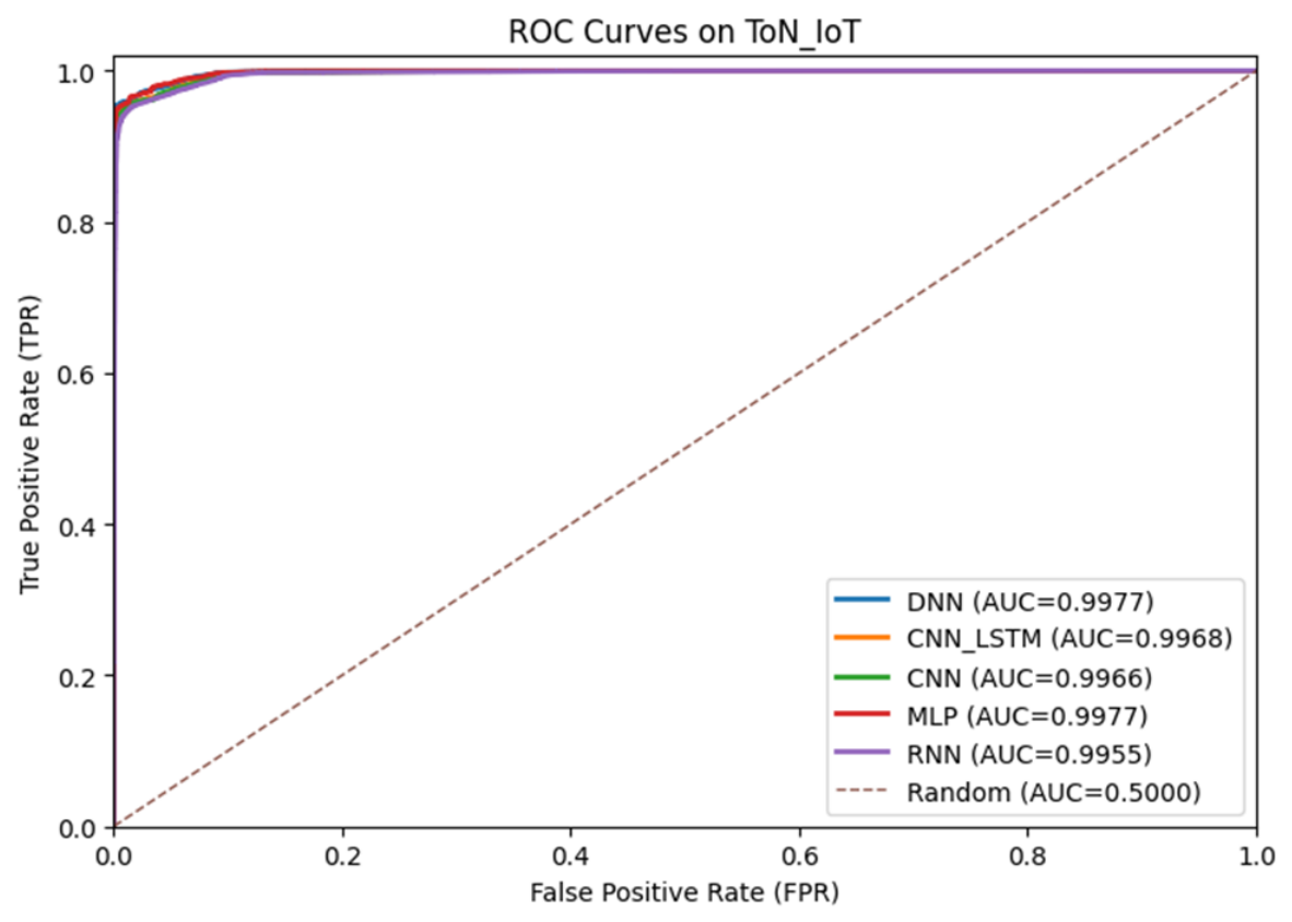
From Figure 4, the ROC curves are grouped closely around the top-left corner (0, 1), which indicates the near-perfect separation of classes obtained by all models. DNN’s curve is slightly higher (ROC-AUC = 0.9977), followed closely by CNN–LSTM (ROC-AUC = 0.9968). The curves have a sharp initial slope, with TPR > 0.95 at FPR < 0.01, which is desirable for operational use, in which security analysts can afford very few false positives while still requiring comprehensive detection of attacks.

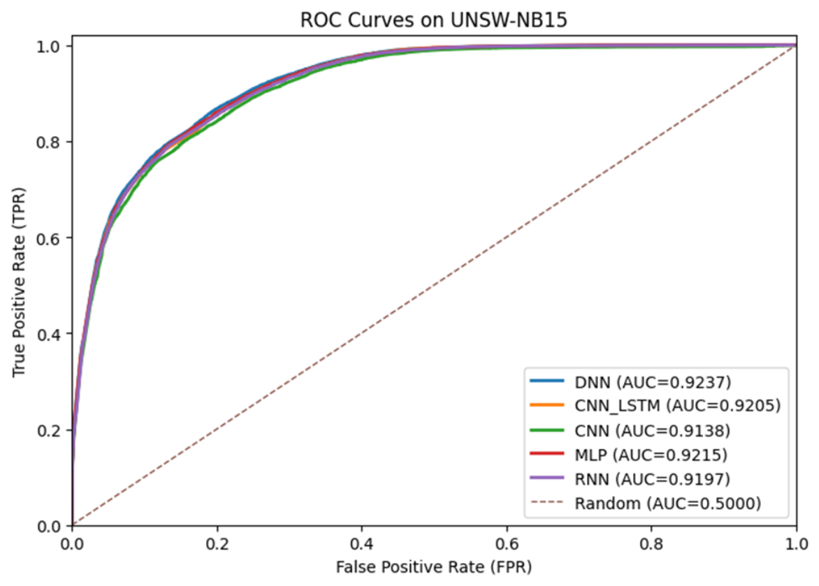
UNSW-NB15 ROC curves in Figure 5 indicate larger separation and departure from the ideal point. DNN achieves the highest ROC-AUC of 0.9237, while the CNN–LSTM model also attains a comparable ROC-AUC of 0.9205, indicating competitive performance. The curves show a less steep rise, requiring FPR values of 0.05 to 0.08 to achieve TPR > 0.95, which is an indication of harder trade-offs between detection and false alarms. This shows that the difficulty level of classification has increased in UNSW-NB15, as the distributions of attack and normal traffic have converged to a large extent.

Analyzing the trade-offs of precision and recall at different thresholds showed that the optimal trade-offs depend on different datasets. Threshold intervals have been found by maximizing the F1-score value obtained from the validation set analysis, verified through ROC curves for an equal balance of true positives and false positives. For ToN_IoT, the most effective threshold intervals are between 0.35 and 0.45, where near-perfect recall and a minimum of false positives is achieved. However, in the case of UNSW-NB15, a greater threshold value is necessary within the interval of 0.50 to 0.60 to reduce the number of false positives while still obtaining a good recall value. Such a comparison indicates the need to examine ROC curves instead of assuming an arbitrary threshold as the optimum.

The DNN outperforms all other models in terms of average accuracy on both datasets, thus reflecting the effectiveness of the network in learning discriminative features. The CNN–LSTM model remains highly competitive and offers a complementary advantage by capturing both spatial feature relationships through convolutional layers and temporal dependencies through recurrent modeling. This hybrid structure provides a more structured and interpretable representation of network traffic behavior, which is particularly relevant for analyzing sequential and multi-stage intrusion patterns.

5. Conclusions

This study has provided a thorough assessment of the proposed CNN–LSTM design in conjunction with four deep learning baselines for IoT intrusion detection on two diverse benchmark datasets. Through a strict experimental design incorporating GWO feature selection, SMOTE class balancing, two-stage scaling, and ROC-based assessment, this paper has thoroughly examined detection capability, the ability to maintain stable performance under different dataset characteristics, and real-world applicability on edge gateways.

From the experimental results, it is evident that all the considered deep learning algorithms were able to perform well across both datasets, with variations in accuracy and ROC-AUC depending on dataset characteristics. These findings suggest that deep learning models can serve as effective baselines for IoT intrusion detection when combined with appropriate preprocessing and feature selection. While the experiment does not aim to demonstrate statistical superiority among the considered deep learning models, the CNN–LSTM architecture remains valuable due to its ability to model both spatial and temporal characteristics of network traffic, offering a more structured and interpretable representation for intrusion detection. This highlights the importance of selecting models not only based on performance but also on their suitability for capturing underlying traffic patterns and supporting practical analysis. It demonstrates high accuracy (99.68% for ToN_IoT and 92.05% for UNSW-NB15) and competitive performance degradation (7.63%), further supporting its robustness across datasets. In addition, the architecture of such models allows interpreting their predictions through the use of convolutions and RNN for the construction of spatial and temporal feature representations of the network traffic, respectively. Thus, the application of such models in IoT settings is justified due to the potential temporal changes in attacks. Despite the increased difficulty of UNSW-NB15, all evaluated models maintain accuracy above 89%, reinforcing the effectiveness of the preprocessing pipeline in producing robust and discriminative feature representations. In particular, the integration of GWO-based feature selection, SMOTE-based class balancing, and dual-stage feature scaling contributes to improved class separability while reducing feature dimensionality and computational overhead, supporting practical deployment. In addition, the analysis of robustness through different datasets suggests that the performance of the models is affected by their specific features, thus pointing out the significance of considering various data environments when assessing intrusion detection systems. Finally, the threshold-aware ROC analysis shows that the optimal operating points are defined based on the requirements of each organization, in which the ToN_IoT dataset can provide the best results at a low false-positive rate, whereas the UNSW-NB15 dataset necessitates trading off with a high false-positive rate because of the greater complexity of the data environment. These findings collectively highlight the importance of combining structured preprocessing, robustness-oriented evaluation, and threshold-aware analysis for developing effective and deployment-ready IoT intrusion detection systems.

Several focused future directions can strengthen practical impact. First, extending the framework to multi-class classification can enable the identification of specific attack categories to support targeted incident response. Second, incorporating federated learning can allow privacy-preserving collaborative training across distributed IoT sites without raw data sharing. Third, improving model transparency through explainability methods, such as attention mechanisms or SHapley Additive exPlanations (SHAP)-based interpretation, can enhance analyst trust and facilitate debugging in operational deployments. It should be noted that the reported differences are based on a single experimental run, and future work will include repeated experiments and statistical significance testing to validate the robustness of these observations. These findings suggest that combining deep learning with a hybrid preprocessing and optimization pipeline yields a more reliable intrusion detection model that can better withstand heterogeneous IoT traffic conditions and support practical edge deployment.