CNN-LSTM-POT-Based Anomaly Detection for Smart Greenhouse Sensor Data: A Real-Time Edge Deployment Approach

Abstract

Traditional agricultural greenhouse environmental monitoring systems often lack effective anomaly detection mechanisms, which can lead to inaccurate environmental regulation and negatively affect plant growth. To address this issue, this paper proposes a greenhouse monitoring system integrating Zigbee and 4G communication technologies, combined with a CNN-LSTM-POT anomaly detection algorithm. The system employs a Convolutional Neural Network (CNN) to extract local spatial features from multi-source sensor data and a Long Short-Term Memory (LSTM) network to model long-term temporal dependencies. To accurately identify anomalies, the Peaks Over Threshold (POT) method from extreme value theory is applied to prediction residuals, enabling adaptive dynamic threshold determination. Experimental results show that the proposed algorithm substantially improves anomaly detection precision, prevents erroneous data from disrupting greenhouse control decisions and reduces the volume of data transmitted to the cloud platform, thereby lowering computational overhead. This work provides a reliable and efficient solution for data monitoring and precise environmental control in smart agricultural greenhouses.

1. Introduction

The rapid growth of the global population has led to an increasing demand for food, requiring a 70% rise in agricultural production to meet projected needs [1,2]. However, traditional approaches to increasing agricultural output, such as expanding arable land, face significant limitations. Approximately 30% of the world’s forests have already been converted to agricultural land [3], and additional land reclamation is increasingly constrained by various political, economic, and environmental factors [4]. Furthermore, recent policy changes and global epidemics have contributed to shortages of agricultural labor, further exacerbating the challenges associated with food production [5,6,7]. Consequently, intelligent agricultural greenhouses have emerged as a promising alternative. These greenhouses help address labor shortages, significantly enhance food production by ensuring optimal growth conditions, improving productivity, and reducing overall production costs [8,9].

Efforts to integrate technology into greenhouse management began in the 1970s, with early adopters recognizing the potential benefits of computerized control systems. By the 1990s, countries such as the United States, Japan, and Israel had further advanced the use of Internet of Things (IoT) technology in agriculture, achieving considerable results. For instance, Japan improved greenhouse efficiency and profitability through microcomputer-based scientific management, whereas Israel effectively addressed water scarcity by integrating drip irrigation with IoT technologies, enabling agriculture even in arid desert regions. Entering the 21st century, research interest and technological advancement in greenhouse systems have continued to grow significantly.

Recent developments have seen numerous research teams creating sophisticated smart greenhouse monitoring and control systems based on IoT and Wireless Sensor Network (WSN) technologies. Ambarwari et al. [10] employed Raspberry Pi and Node-RED for highly reliable environmental data collection and visualization, achieving a storage success rate of 99.76%. Jahnavi et al. [11] developed automated greenhouse control using ZigBee protocols. Madruga-Peláez et al. [12] introduced a low-power wireless sensor network focusing on optimized energy consumption of sensor nodes. Pisanu et al. [13] proposed a low-cost monitoring platform integrating multiple sensor modules, supporting both wired and wireless data transmission as well as web-based visualization. Furthermore, Shekarian et al. [14] utilized artificial intelligence (AI) techniques, specifically employing a 1D-CNN model, to enhance sensor fault detection and predictive accuracy. These studies collectively illustrate the potential of precision agriculture and provide pathways toward automated control and crop-specific optimizations.

Despite advancements in IoT-based greenhouse systems, sensor data anomalies remain a persistent issue, occurring due to network disruptions, sensor faults, or human-induced disturbances. Such anomalies, if undetected, can compromise the accuracy and reliability of the automated decision-making processes integral to greenhouse management. Therefore, effective integration of anomaly detection algorithms into greenhouse monitoring systems is critical for maintaining data integrity and supporting precise environmental control.

To address these challenges, this paper introduces a novel greenhouse monitoring system that integrates a robust anomaly detection algorithm. The proposed system utilizes an edge-based CNN-LSTM-POT model to perform anomaly detection at the gateway level, effectively filtering erroneous data before transmission. This not only enhances the reliability of automated greenhouse management decisions but also significantly reduces data traffic to cloud-based platforms, thereby decreasing computational and bandwidth demands.

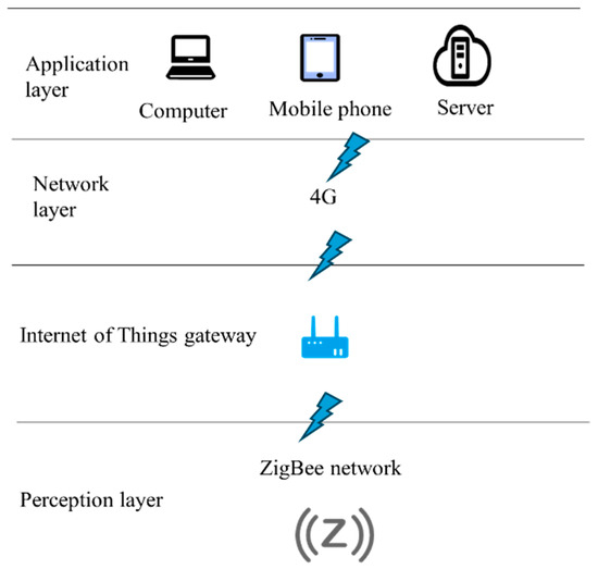
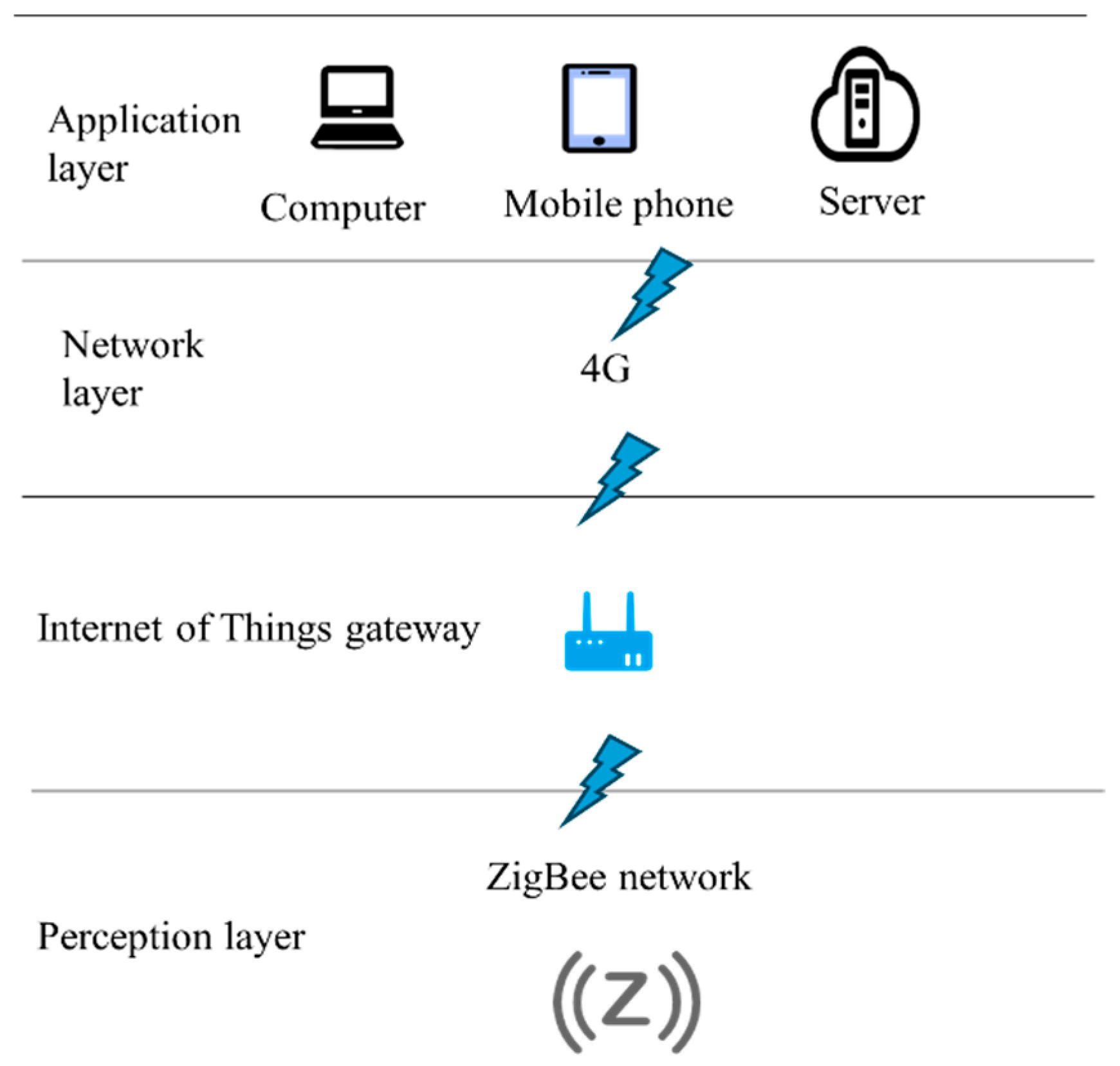
The architecture of the greenhouse monitoring system proposed in this paper is depicted in Figure 1. The developed monitoring system includes sensors to collect real-time environmental parameters such as temperature, humidity, and illumination. A microcontroller-based data acquisition module (STM32F103C8T6) initially processes sensor data and transmits it via Zigbee modules to a coordinator, which then forwards data to a gateway (STM32H743-based). The gateway implements the proposed anomaly detection algorithm to identify and remove anomalous data points, thus ensuring data quality. Subsequently, validated data is transmitted to a cloud platform using a built-in 4G communication module. Users can remotely access and monitor environmental conditions in real-time, enabling timely interventions and informed decision-making.

The remainder of this paper is structured as follows: Section 2 reviews existing methods and concepts related to anomaly detection. Section 3 provides a comprehensive explanation of the proposed anomaly detection algorithm. Section 4 evaluates the algorithm’s performance, demonstrating its effectiveness through experimental analysis. Section 5 discusses practical implementation details of the algorithm within the gateway, including experiment setups and parameter settings. Finally, Section 6 summarizes the contributions of this research, highlights key findings, and outlines potential directions for future work.

2. Related Work

In wireless sensor networks, anomalous data transmission or reception can be caused by various factors, including sensor malfunctions, battery depletion or voltage instability (resulting in data jumps or losses), signal attenuation caused by node movement or physical obstructions, and external environmental conditions such as high temperature or humidity. Such anomalous data poses significant risks to smart greenhouse operations, potentially leading to incorrect control decisions and adverse effects on crop growth. Hence, incorporating effective anomaly detection algorithms into greenhouse gateways is essential for ensuring data reliability and system robustness.

Anomaly detection techniques generally fall into three main types: statistical-based, deviation-based, and proximity-based methods [15].

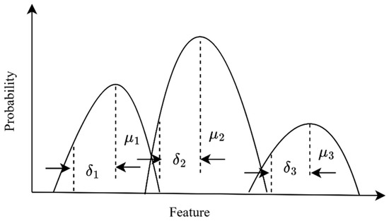
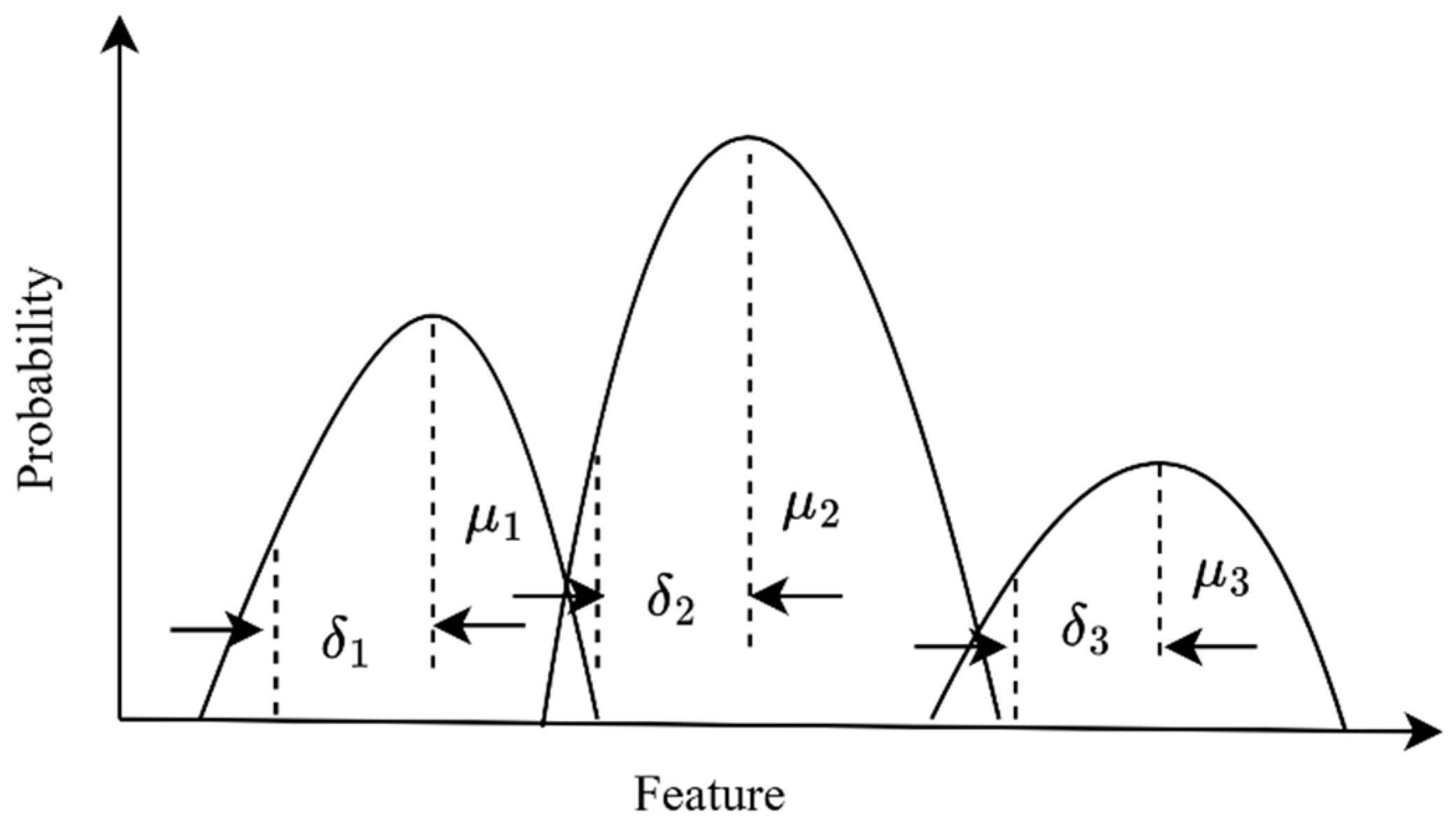
Statistical-based methods: These approaches assume that the data conform to a certain probability distribution. Observations that deviate substantially from the expected distribution are treated as anomalies. A prominent example is the Gaussian Mixture Model (GMM), which presumes that the data originates from a mixture of several Gaussian distributions, each characterized by its own mean and variance. The model estimates the probability of each data point belonging to these distributions and flags points with low likelihoods as anomalies. An illustration of this approach is provided in Figure 2.

Deviation-based methods: These approaches quantify the extent to which a data instance deviates from a predefined distribution model or subspace structure to identify significant outliers. A representative example is Principal Component Analysis (PCA), which reconstructs the original data using only a few principal components. Data points that exhibit large reconstruction errors are considered anomalous.

Proximity-based methods: These techniques evaluate the spatial relationships among data points and can be further subdivided into three categories: clustering-based, density-based, and distance-based methods.

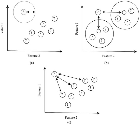
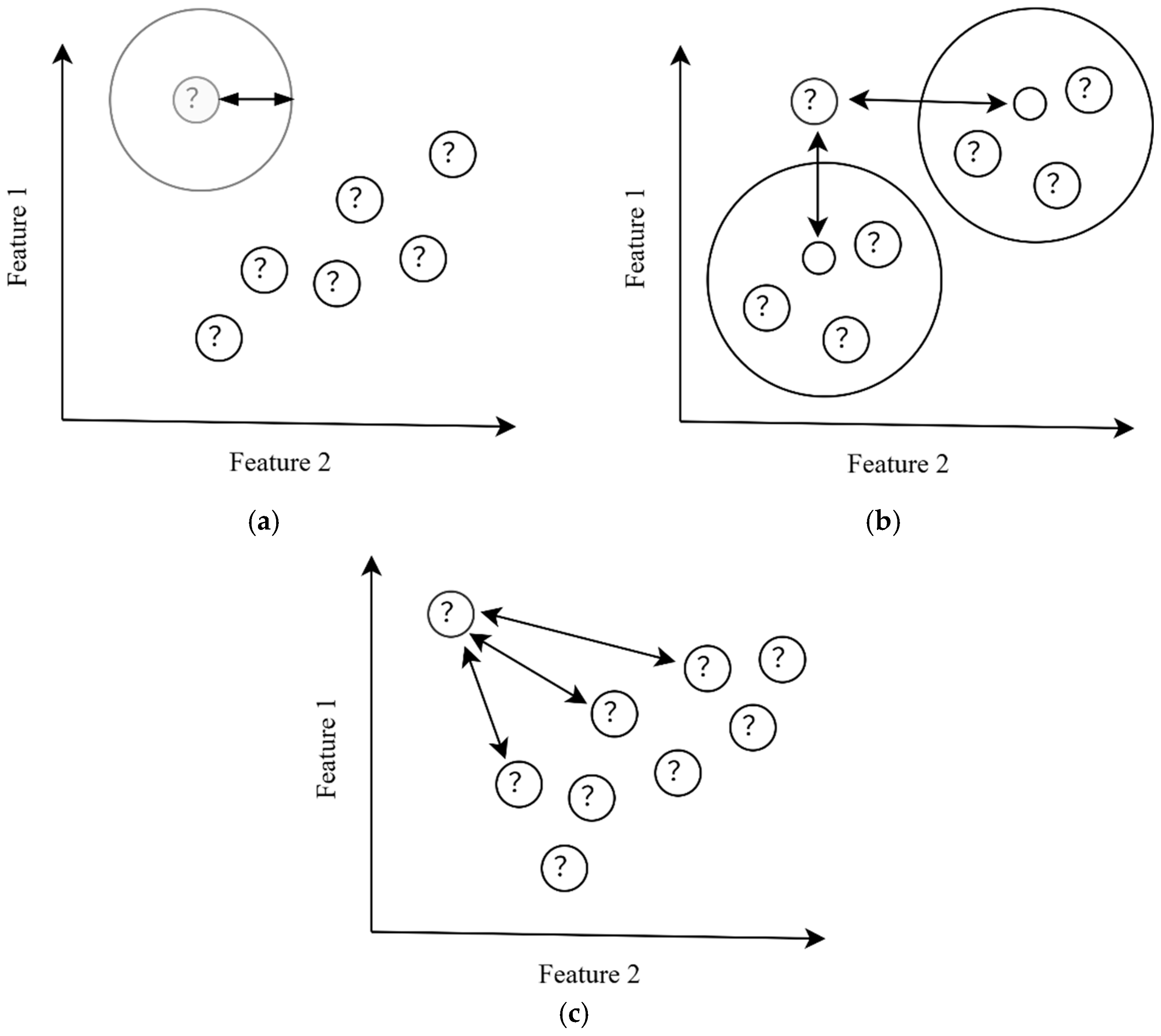
Clustering-based: Data points are grouped into clusters, and those that do not belong to any cluster are flagged as anomalies. The classification is typically based on the distance between the data point and the cluster centroids, as illustrated in Figure 3a.

Density-based: The local density surrounding a data point is computed, and points with significantly lower densities than their neighbors are identified as anomalies. This approach is depicted in Figure 3b.

Distance-based: Data points that lie at a considerable distance from their nearest neighbors are classified as anomalies. This concept is shown in Figure 3c.

To overcome the limitations of traditional techniques, recent studies have introduced a range of innovative algorithms, particularly targeting the complexities of time-series and multi-sensor data.

Zhang et al. [16] proposed an anomaly detection algorithm for Wireless Sensor Networks (WSNs) based on Power Line Communication (PLC), addressing challenges associated with the unique deployment characteristics, openness, and resource constraints of WSNs. The algorithm analyzes time-series data and integrates graph signal processing with clustering techniques to efficiently detect and localize both local and global anomalies. Experimental results demonstrate high detection accuracy and effectiveness in reducing communication overhead within the network.

Nesrine et al. [17] introduced a spatio-temporal (ST) and multivariate attribute (MVA) correlation-based method to detect anomalous nodes in WSNs. The method analyzes both intra-cluster and inter-cluster spatio-temporal correlations in homogeneous sensor data and incorporating environmental context through multivariate attribute rules, the approach effectively distinguishes real-world events from anomalies such as malicious attacks or sensor failures. Experiments on real-world datasets confirmed its ability to accurately capture sensor data relationships and identify faulty nodes, thereby reducing false alarms and improving overall system reliability.

Kruthi et al. [18] presented a clustering and deep learning-based approach for detecting anomalies in multivariate gas sensor data. The method targets high-precision anomaly detection in complex scenarios and evaluates various unsupervised learning algorithms on real-world datasets. The results show that density-based clustering achieves superior performance in detecting both global and local anomalies.

Hyunki et al. [19] developed a Generative Adversarial Network (GAN)-based framework for detecting and localizing anomalies in multivariate time-series data. The approach transforms time-series data into distance images, then applies pointwise convolution to extract temporal information and traditional convolution to capture spatial correlations across variables. The generator learns the normal data distribution to predict future distance images, while an anomaly scoring function—defined using reconstruction loss and discriminator feature loss—facilitates anomaly detection and localization. The framework was validated on real-world power plant data, demonstrating its effectiveness in identifying anomalous events and faulty sensors.

Wataru et al. [20] proposed a machine learning-based method for detecting abnormal vehicle vibrations. Using piezoelectric sensors installed on vehicle bodies, vibration data is collected and analyzed through feature extraction techniques such as Power Spectral Density (PSD) and Mel-Frequency Cepstral Coefficients (MFCC). Classification is performed using Gaussian Mixture Models and Convolutional Neural Networks.

Hu et al. [21] introduced a data-driven ensemble framework for anomaly detection and early warning in Water Distribution Systems (WDS). The framework comprises four modules: single-point anomaly detection, sensor sequence analysis, inter-sensor sequence correlation, and a qualitative analysis component. By incorporating spatio-temporal characteristics of monitoring data, the framework significantly enhances anomaly detection reliability and operational efficiency, supporting clean and sustainable water system management.

Mingu et al. [22] proposed an unsupervised anomaly detection method based on channel-wise reconstruction errors in multi-channel sensor signals. A Convolutional Autoencoder (CAE) is used to generate reconstruction errors for each channel, which are then input into machine learning-based anomaly detection models to compute anomaly scores. Simulation and real-world experiments on automotive sensor data confirm the method’s effectiveness. Compared with traditional approaches relying solely on average reconstruction error, this method significantly improves anomaly detection accuracy, especially in low-anomaly-rate conditions.

Clementine et al. [23] proposed an anomaly detection framework for agricultural IIoT. Addressing the challenges of device heterogeneity and unstable networks in agriculture, the framework adopts unified communication protocols to ensure device interoperability and introduces edge/fog computing architectures for processing data near the source. By deploying machine learning algorithms like Isolation Forest, Autoencoders, and LSTM at the edge layer, it enables real-time anomaly identification from crop and environmental data, reducing transmission latency and cloud dependence. This approach allows farmers to receive timely crop health alerts, facilitating rapid intervention and precise decision-making, thereby improving agricultural production efficiency and resource utilization.

While these methods have achieved some results, several research gaps remain in the context of smart greenhouse environments. First, many existing approaches are computationally intensive and require substantial resources, making them unsuitable for deployment on resource-constrained edge devices such as greenhouse gateways. Second, most methods rely on static thresholds for anomaly detection, which struggle to adapt to the non-stationary nature of greenhouse sensor data.

To address these gaps, this paper proposes a CNN-LSTM-POT-based anomaly detection framework specifically designed for edge deployment in smart greenhouse monitoring systems. The main innovations of this work are as follows:

Lightweight hybrid architecture: The proposed model combines a CNN for local feature extraction and LSTM for temporal modeling, ensuring high prediction accuracy while maintaining computational efficiency suitable for edge devices.

POT-based adaptive thresholding: Unlike fixed-threshold methods, the POT module dynamically adjusts the anomaly threshold based on the statistical distribution of prediction residuals, enabling robust detection in non-stationary environments.

By explicitly addressing the challenges of computational constraints and dynamic data characteristics, the proposed CNN-LSTM-POT method provides a practical solution for anomaly detection in smart agricultural greenhouses.

3. Anomaly Detection Algorithm Framework

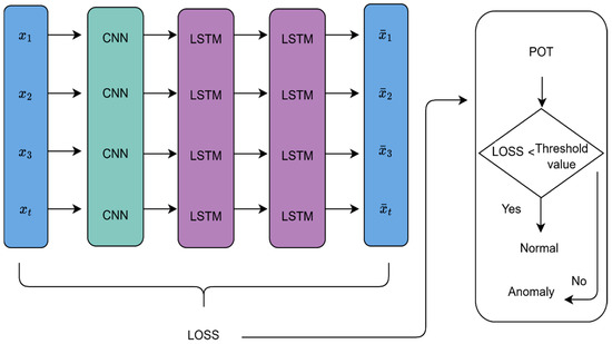
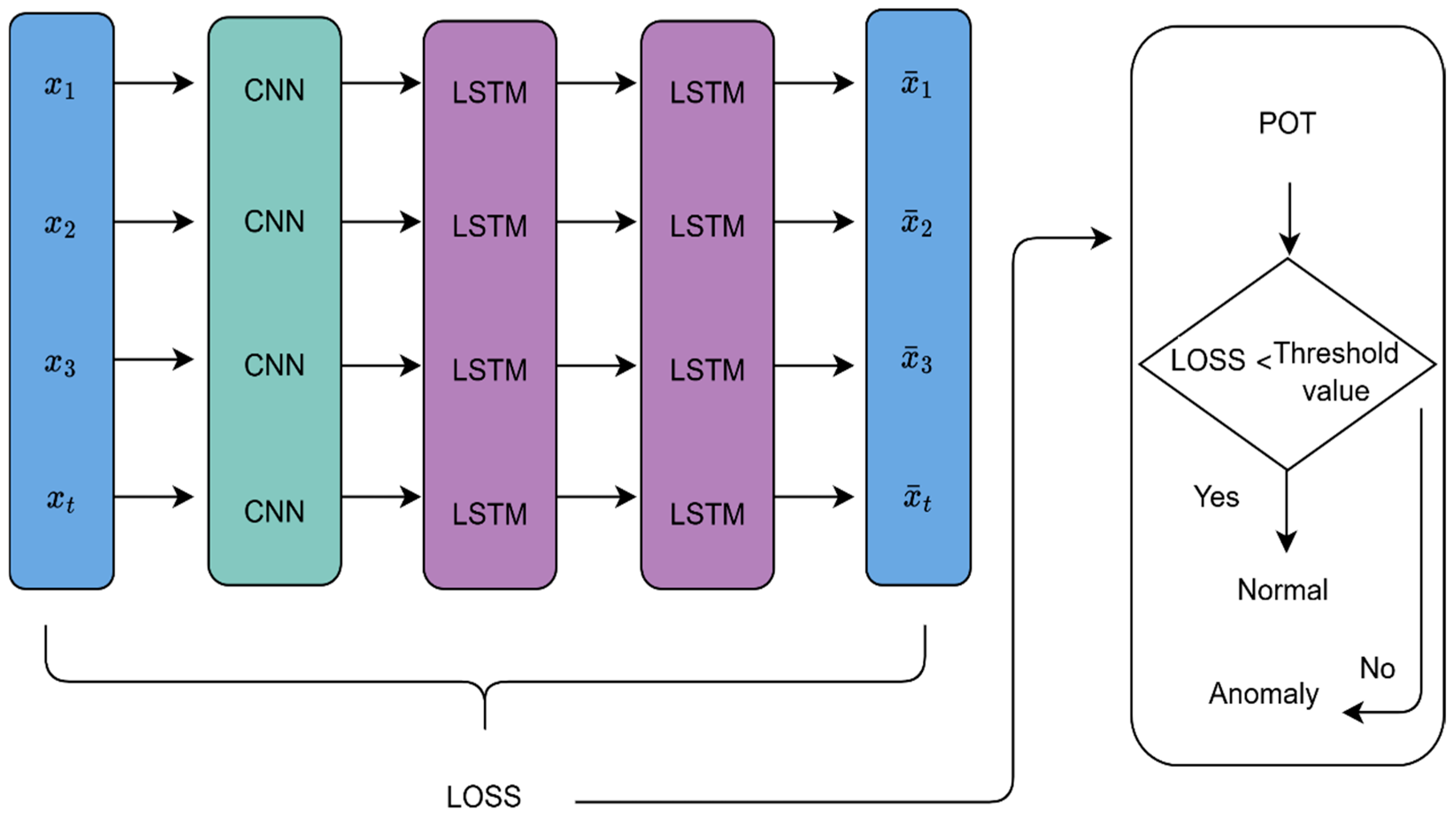
This paper proposes a novel anomaly detection algorithm for greenhouse environmental monitoring data, which integrates a CNN, a LSTM network, and the POT method—collectively referred to as the CNN-LSTM-POT model. The algorithm first predicts future sensor values using a CNN-LSTM structure and then applies extreme value theory through the POT method to dynamically determine an anomaly threshold. If the prediction residual—defined as the deviation between the actual and predicted values—exceeds this threshold, the corresponding data point is classified as anomalous; otherwise, it is treated as normal.

To facilitate real-time detection, the algorithm incorporates a sliding window mechanism that enables real-time modeling and prediction using historical data. Specifically, a fixed-length sliding window of size N is used, which advances continuously with time. At each step, only the most recent N data points are used for model computation and anomaly determination. The full anomaly detection process is illustrated in Figure 4 and formalized in Algorithm 1.

In real-world scenarios, sensor data from different sources may vary in unit scales and numerical ranges. Directly feeding such data into the model may impair training convergence and prediction accuracy. To address this, min–max normalization is applied to the raw data before prediction, using the following equation:

$$x^{\prime }={\displaystyle \frac{x-x_{min}}{x_{max}-x_{min}}}$$

(1)

where $x$ is the original input value, $x^{\prime }$ is the normalized value, and $x_{min}$ and $x_{max}$ are the minimum and maximum values observed in the current sliding window, respectively. When new data points arrive outside the previously observed range, the normalization parameters $x_{min}$ and $x_{max}$ are dynamically updated based on the values within the current sliding window. This ensures that the normalization remains adaptive to evolving data distributions without requiring global statistics, thereby maintaining consistency and comparability across time steps.

Algorithm 1: CNN-LSTM with POT-based Anomaly Detection

Input: Sensor data sequence X = {$x_1$, $x_2$, …, $x_t$}

Output: Anomaly detection result

1: For each time step $t$ extract input features within a sliding window: $X_{window}$ 2: Extract local spatial features: $feature{s}_{CNN}=CNN\left(X_{window}\right)$ 3: Model temporal dependencies: ${hidden}_{state}=LSTM\left(feature{s}_{CNN}\right)$ 4: Predict the expected sensor value: ${\widehat{x}}_t=FullyConnectedLayer\left({hidden}_{state}\right)$ 5: Compute prediction error: $e_t={\left|\left|x_t-{\widehat{x}}_t\right|\right|}^2$ 6: Maintain sliding window of recent errors: ${\epsilon }_t=\{e_{t-N+1},\dots ,e_t\}$ 7: Fit Generalized Pareto Distribution (GPD) to exceedances over a initial threshold $u$: $GPD(e_i-u|e_i>u)$ 8: Compute the dynamic anomaly threshold $\tau$ at $(1-\alpha )$ quantile 9: Determine anomaly condition: if $e_t>\tau$, label $x_t$ as anomalous

To further improve the generalization performance and mitigate overfitting, regularization techniques [24] are integrated into the training phase. These strategies enhance the model’s robustness and adaptability under varying environmental conditions.

In the aforementioned algorithm, ${\epsilon }_t$ denotes the error set within the current window, $\tau$ is the dynamic anomaly threshold, $N$ is the size of the sliding window, $\alpha$ is the significance level representing the false positive rate, and $u$ represents the initial threshold

3.1. CNN-LSTM Anomaly Prediction Model Framework

A CNN is a feedforward neural network characterized by local connectivity and shared weights [25]. In the context of time series modeling, CNNs are highly effective in extracting local patterns and high-level features from input data, thereby providing more informative and discriminative representations for subsequent processing by the LSTM network. This layered approach enhances the model’s overall prediction accuracy [26].

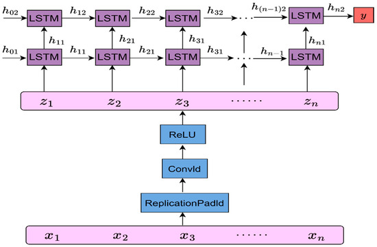
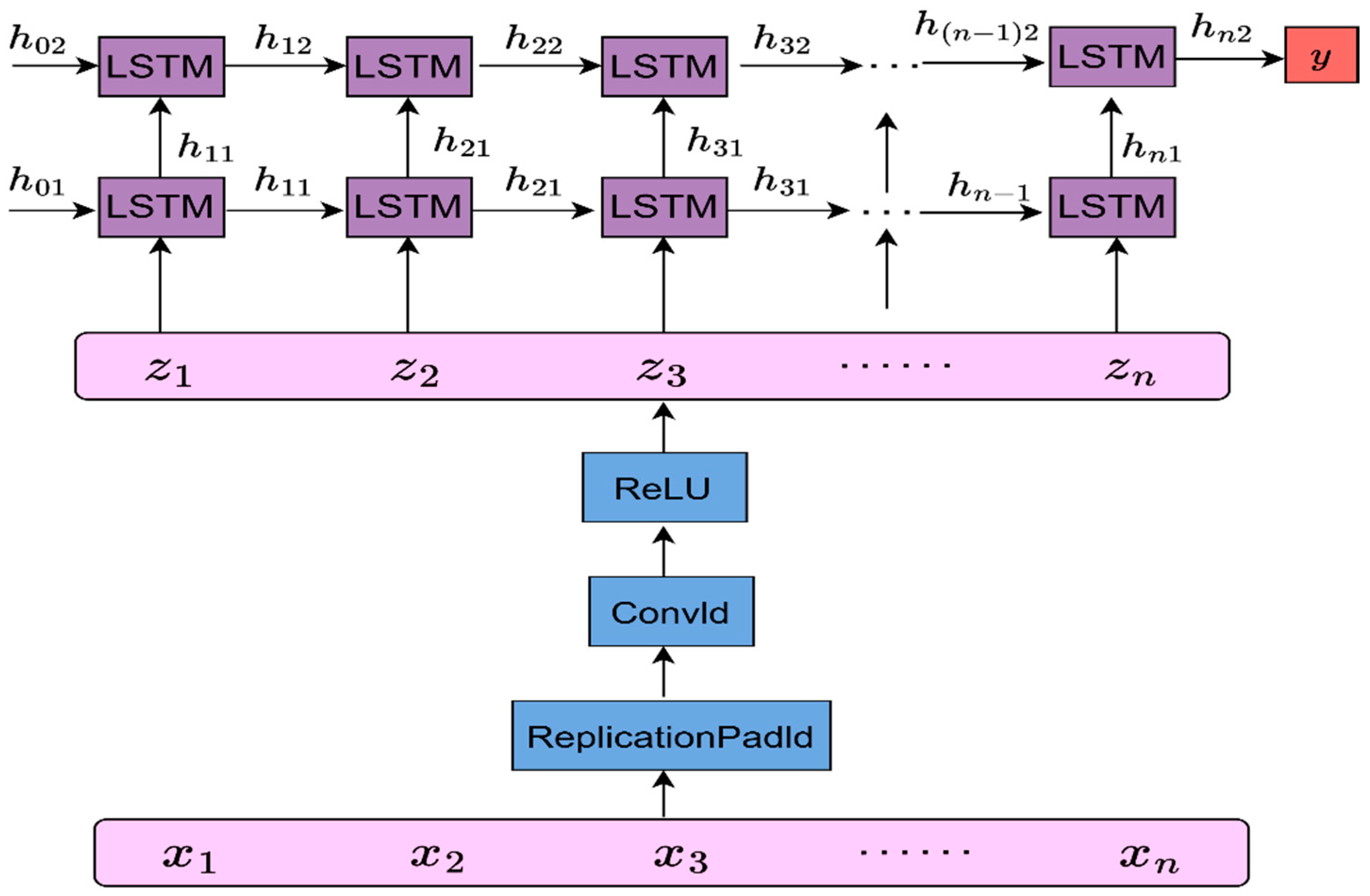
As illustrated in Figure 5 and Algorithm 2, the input time series X first undergoes one-dimensional convolution to extract features, resulting in a high-order feature matrix $Z=(z_1,z_2,\dots ,z_n)$, where each feature vector $z_t=(z_{t1},z_{t2},\dots ,z_{tn})$ represents the activation values across $n$ feature channels at time $t$.

Algorithm 2: Data Prediction Based on CNN-LSTM

Input: Normalized time series data X

Output: Predicted sensor value y

1: Feature Extraction: Compute the high-order feature matrix Z using Equation (2) 2: LSTM initialization: Initialize the hidden states of the LSTM layers 3: Temporal modeling: Use Equation (3) to compute the hidden state $h_{n1}$ in the first LSTM layer Use Equation (4) to compute the hidden state $h_{n2}$ in the second LSTM layer 4: Prediction output: Apply a linear transformation to $h_{n2}$ using Equation (5) to obtain the predicted value $y$

In the convolution layer, the input sequence $X$ is first padded using the ReplicationPad1d method to maintain dimensional consistency at the boundaries. Then, one-dimensional convolution is applied as described by the following equation:

$$Z=ReLU(W\otimes X+b)$$

(2)

Here, ReLU denotes the activation function, and $\otimes$ represents the cross-correlation operator. $W$ is a three-dimensional convolution kernel tensor, and $b$ is the bias vector.

The resulting feature sequence $Z$ is then passed into the LSTM network for temporal modeling. The first-layer LSTM unit takes the current input $z_n$ and the previous hidden state $h_{n-1}$, and computes the current hidden state $h_{n1}$ as follows:

$$h_{n1}=f(h_{n-1},z_n)$$

(3)

where $f(·)$ represents the forward propagation function of the LSTM unit.

Next, the second-layer LSTM unit computes the hidden state $h_{n2}$ using the previous hidden state $h_{\left(n-1\right)2}$ and the current moment’s hidden state $h_{n1}$ of the first layer:

$$h_{n2}=f(h_{\left(n-1\right)2},h_{n1})$$

(4)

Finally, the model generates the predicted output $y$ by applying a linear transformation to the second-layer hidden state:

$$y=V{h}_{n2}$$

(5)

where $V$ is the linear transformation weight vector.

3.2. Anomaly Decision Process

During the anomaly detection process, real-time sensor data is continuously fed into the active sliding window, and a prediction residual is computed for each data point. To enable precise discrimination of anomalous observations, this study employs the POT method [27] to dynamically determine the detection threshold. Unlike traditional methods that rely on a fixed threshold, POT leverages extreme value theory (EVT) by modeling exceedances above a baseline threshold using the GPD, thereby enabling adaptive thresholding that reflects the actual statistical properties of the data.

The cumulative distribution function (CDF) of the GPD is given by:

$$\overline{F}\left(s\right)=P(S-m>s|m<S)~{(1+{\displaystyle \frac{\gamma s}{\beta }})}^{-{\displaystyle \frac{1}{\gamma }}}$$

(6)

In Equation (6), $S$ represents the prediction residual (the difference between the predicted value and the actual value), $m$ is the initial threshold, $\gamma$ is the shape parameter of the distribution function, and $\beta$ is the scale parameter of the distribution function.

The final dynamic threshold $w$ can be estimated using the inverse cumulative distribution function of GPD:

$$w\simeq m+{\displaystyle \frac{\widehat{\beta }}{\widehat{\gamma }}}({\left({\displaystyle \frac{qN}{G}}\right)}^{-\widehat{\gamma }}-1)$$

(7)

where $m$ is the initially set reference threshold, $\widehat{\gamma }$ and $\widehat{\beta }$ are the shape and scale parameters estimated via Maximum Likelihood Estimation (MLE), $q$ is the desired anomaly proportion, $N$ is the size of the sliding window, and $G$ is the actual number of abnormal samples exceeding $m$.

This dynamic thresholding mechanism allows the system to flexibly and accurately detect sudden or high-magnitude anomalies, improving both the adaptability and robustness of the anomaly detection algorithm in complex and noisy environments. In this study, the POT method is configured with a quantile threshold of 0.99 to determine the initial threshold $m$, and a significance level of $q={10}^{-4}$. The specific implementation is described in Algorithm 3.

Algorithm 3: POT-based anomaly detection

Input: Reconstruction error sequence within the sliding window

Output: Anomaly flag

1: Set the initial threshold $m$ based on empirical observations 2: Maintain a sliding window to store recent reconstruction errors 3: Extract the subset of errors that exceed the threshold $m$ 4: Count the number of exceedances, denoted as $G$ 5: Estimate the expected anomaly proportion $q$ 6: Use MLE to fit a GPD to the exceedance values, obtaining $\widehat{\gamma }$ and the scale parameter $\widehat{\beta }$, Compute the dynamic threshold $w$ using Equation (7) 7: If the current reconstruction error $e_t>w$, flag the corresponding data point as an anomaly

3.2.1. Sensitivity Analysis of POT Parameters

To further validate the robustness of the proposed method and provide practical guidance for parameter selection in real-world greenhouse environments, we conducted a sensitivity analysis on two key parameters of the POT method: the quantile threshold and the significance level $q$.

As shown in

Table 1. Sensitivity analysis results for quantile threshold.

Quantile Threshold	F1-Score (%)
0.90	88.6
0.95	90.1
0.98	91.6
0.99	92.2
0.995	91.5
0.999	84.8

, the F1-score improves from 88.6% to 92.2% as the quantile increases from 0.90 to 0.99, due to better focus on extreme residuals. However, when the quantile exceeds 0.995, the F1-score drops to 91.5% and further to 84.8% at 0.999, indicating that an excessively high quantile degrades detection performance.

The results in

Table 2. Sensitivity analysis results for significance level q.

Significance Level (q)	F1-Score (%)
${10}^{-2}$	86.0
${10}^{-3}$	92.6
${10}^{-4}$	92.2
$5\times {10}^{-5}$	90.4
${10}^{-5}$	82.8

indicate that setting q too low leads to a lower F1-score of 82.8% due to missed anomalies, while setting q too high yields an F1-score of 86.0% due to increased false positives. The optimal F1-scores are achieved when q is between ${10}^{-4}$ and ${10}^{-3}$, balancing precision and recall across various greenhouse conditions.

Based on the sensitivity analysis, we provide the following practical recommendations for deploying the CNN-LSTM-POT model under different greenhouse environments:

For stable greenhouse environments, a higher quantile (0.995) and a lower $q$ ($5\times {10}^{-5}$) are recommended to minimize false alarms while capturing rare but critical anomalies.

For dynamic greenhouse environments, a moderate quantile (0.98–0.99) and a higher $q$ (${10}^{-3}$) are more suitable to maintain sensitivity to anomalies without being overwhelmed by noise.

For unknown or mixed environments, we suggest starting with default values (quantile = 0.99, $q={10}^{-4}$) and fine-tuning based on a small validation set with labeled anomalies or domain expert feedback.

3.2.2. Impact of the Sliding Window on Detection Delay and Accuracy

The choice of sliding window size N directly impacts the detection delay and the algorithm’s sensitivity. A smaller N allows the model to adapt more quickly to changes in the data distribution, leading to lower detection delays for anomalies. However, it also means the model is trained on less data, making it potentially more susceptible to noise and resulting in a less stable estimation of the POT. Conversely, a larger N provides more historical data, leading to a more robust and stable model and threshold estimation, but it also increases the detection delay because the model responds more slowly to new trends and may be slower to identify anomalies emerging from a new baseline. The optimal N is therefore a trade-off and should be selected based on the specific requirements of the greenhouse application, balancing the need for rapid detection against the tolerance for false alarms.

4. Algorithm Performance Evaluation

The CNN-LSTM-POT anomaly detection model utilizes a carefully selected set of hyperparameters to balance model complexity, computational efficiency, and detection accuracy. The architecture consists of a 1D convolutional layer (Conv1D) with 32 filters and a kernel size of (3, 1), followed by two LSTM layers employing the tanh activation function and a dropout rate of 0.2 to prevent overfitting. The model is trained using the Adam optimizer with a mean squared error (MSE) loss function, a batch size of 64, and 30 training epochs.

4.1. Configuration and Calibration of Baseline Models

To establish a rigorous and equitable evaluation framework, all baseline models—namely LSTM, Beat Generative Adversarial Network (BeatGAN), and Temporal Hierarchy One-Class (THOC)—were compared with the proposed CNN-LSTM-POT model under strictly controlled conditions. This was achieved by standardizing three key aspects of the experimental setup: dataset partitioning, hyperparameter optimization, and anomaly threshold determination.

First, to ensure temporal consistency and result comparability, all models were trained and evaluated on the same dataset splits. The data were chronologically divided into training (70%), validation (15%), and test (15%) sets, thereby preserving the sequential structure of the time series and preventing data leakage.

Second, to guarantee that each model operated at its optimal capacity, hyperparameter tuning was conducted uniformly via grid search, with the objective of maximizing the F1-score on the validation set. The resulting optimal configurations for each baseline model are summarized in

Table 3. Hyperparameter configurations of baseline models.

Model	Hyperparameters	Search Range	Optimal Value
LSTM	Hidden units	[32, 64, 128]	64
	Number of layers	[1, 2, 3]	2
	Dropout rate	[0.1, 0.2, 0.3]	0.2
	Learning rate	[0.001, 0.01, 0.1]	0.001
BeatGAN	Latent dimension	[16, 32, 64]	32
	Generator layers	[2, 3, 4]	3
	Discriminator layers	[2, 3, 4]	3
	Adversarial weight	[0.1, 0.5, 1.0]	0.5
THOC	Temporal window	[10, 20, 50]	20
	Dilations	[[1, 2, 4], [1, 2, 4, 8]]	[1, 2, 4, 8]
	One-class margin	[0.1, 0.5, 1.0]	0.5
	Hidden channels	[32, 64, 128]	64

.

Third, to enable fair assessment of detection sensitivity, the thresholding strategies were carefully aligned with the adaptive POT mechanism used in the proposed method. For reconstruction error-based models such as LSTM and BeatGAN, a quantile-based threshold was derived from the validation error distribution, corresponding to the significance level of $q={10}^{-4}$ employed in the POT approach. For the THOC model, the one-class margin threshold recommended in its original study was adopted and subsequently fine-tuned on the validation set to optimize performance.

By harmonizing these critical experimental factors, the comparison across models becomes both transparent and meaningful, providing a solid foundation for evaluating the relative effectiveness of the proposed anomaly detection framework.

4.2. Evaluation Indicators

To evaluate the prediction accuracy of the CNN-LSTM model, the Mean Absolute Error (MAE) is adopted as the primary performance metric. The MAE is computed using the following equation:

$$MAE={\displaystyle \frac{1}{n}}{\sum }_{i=1}^n|X_i^{\prime }-X_i|$$

(8)

where $n$ is the total number of samples, $X_i^{\prime }$ is the predicted value, and $X_i$ is the actual value.

To assess the algorithm’s real-time anomaly identification capability, three commonly used classification metrics are employed: Precision, Recall, and F1-score [28]. These are defined as follows:

$$Precision={\displaystyle \frac{True Positive}{True Positive+False Positive}}$$

(9)

$$Recall={\displaystyle \frac{True Positive}{True Positive+False Negative}}$$

(10)

$$F_1={\displaystyle \frac{2\times Precision\times Recall}{Precision+Recall}}$$

(11)

In Equations (9)–(11):

True Positive (TP): Number of correctly identified anomalous samples.

False Positive (FP): Number of normal samples incorrectly labeled as anomalies.

False Negative (FN): Number of anomalous samples incorrectly labeled as normal.

To conduct statistical significance tests for the model, the mean difference, t-statistic, and p-value are introduced. These are defined as follows:

$$\overline{d}={\displaystyle \frac{\sum _{i=1}^n{d}_i}{n}}$$

(12)

where $\overline{d}$ is mean difference, $d_i$ is difference between the two models in the i-th run, $n$ is number of independent runs.

$$t={\displaystyle \frac{\overline{d}\times \sqrt{n}}{s_d}}$$

(13)

$$s_d=\sqrt{{\displaystyle \frac{\sum _{i=1}^n{(d_i-\overline{d})}^2}{n-1}}}$$

(14)

where $t$ is t-statistic, $s_d$ is standard deviation of the differences.

$$p=2\times P(T_{df}>|t\left|\right)$$

(15)

where $p$ is p-value, $T_{df}$ is t-distribution with df degrees of freedom.

To test the anomaly recognition capability of the gateway, the recognition rate was introduced.

The recognition rate is computed using the following equation:

$$Recognition Rate={\displaystyle \frac{Total Data Points-Data Transmitted via Gateway}{Total Anomaly Data Points}}\times 100\%$$

(16)

Total Data Points: All data points collected during the experiment.

Data Transmitted via Gateway: The number of clean data points uploaded to the cloud after filtering by the algorithm.

Total Anomaly Data Points: The total number of anomalous data points intentionally introduced in the experiment.

By conducting a comprehensive analysis based on these evaluation metrics, the performance of the proposed anomaly detection algorithm can be quantitatively assessed and benchmarked against existing methods. This enables verification of its effectiveness and robustness in practical greenhouse monitoring scenarios.

4.3. Statistical Significance Testing

To rigorously validate the performance advantages of the proposed CNN-LSTM-POT model, we conducted statistical significance tests. Each model was independently run 10 times with different random seeds, and the resulting F1 scores were recorded. Paired t-tests were then performed to compare the proposed model against each baseline model. The specific details can be found in

Table 4. Statistical significance test results.

Comparison Model	Mean Difference	T-Statistic	p-Value
LSTM	0.02	3.15	<0.01
BeatGAN	0.13	14.23	<0.001
THOC	0.05	5.89	<0.01

.

The results in Table 4 demonstrate that the performance gains of the proposed model are statistically significant (p < 0.05) relative to all three baseline methods, confirming that the observed improvements are not attributable to random variation.

4.4. Loss Assessment

To thoroughly evaluate the training dynamics and generalization capability of the proposed CNN-LSTM model, this section provides a detailed analysis of the loss curves, training configuration, and overfitting prevention strategies employed.

The model was trained using the Adam optimizer at an initial learning rate of 0.001. This learning rate was chosen based on preliminary experiments balancing convergence speed and stability; it allows the model to descend efficiently along the loss landscape without oscillating or diverging. A batch size of 64 was used to provide stable gradient estimates while maintaining computational efficiency. The dataset was chronologically split into training (70%), validation (15%), and test (15%) sets, preserving temporal continuity and preventing data leakage. The validation set was used exclusively to monitor model performance on unseen data during training.

To mitigate the risk of overfitting, dropout regularization was incorporated into the training pipeline: a dropout rate of 0.2 was applied after each LSTM layer. This technique randomly deactivates 20% of the neurons during training, forcing the network to learn more robust and distributed representations rather than relying on specific neurons.

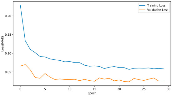
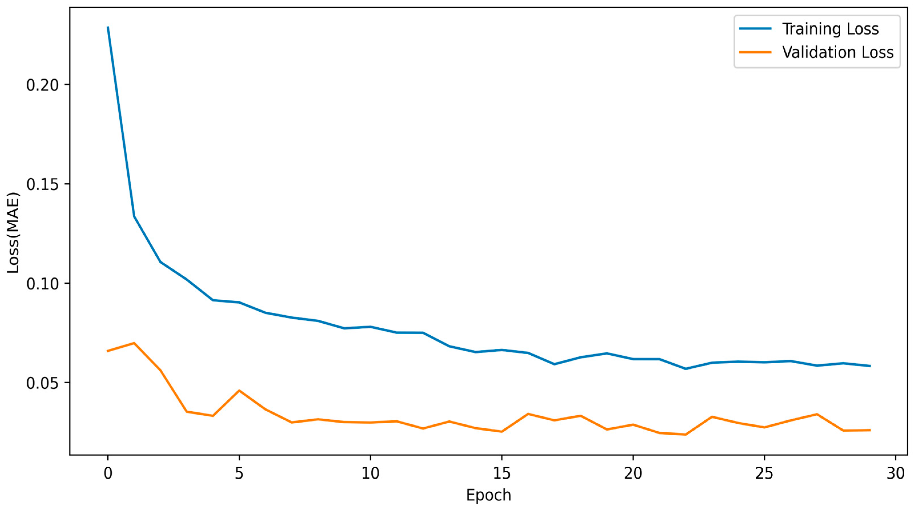
Figure 6 shows the training and validation loss curves over 30 training epochs. Both curves begin at a relatively high initial value of approximately 0.225 and decrease in parallel, eventually converging at around 0.025. The consistent alignment between the two curves throughout the training process indicates a stable and effective learning trajectory, with no signs of overfitting. This close tracking confirms that the dropout regularization successfully prevented the model from diverging from the validation data distribution.

During the initial 10 epochs, the loss values decrease rapidly, suggesting that the model quickly captures the fundamental patterns in the data. After this initial phase, the loss values enter a gradual refinement stage, where the model fine-tunes its features while maintaining generalization. The absence of a diverging validation loss confirms the effectiveness of the adopted regularization strategy.

Overall, the loss curves demonstrate strong convergence behavior, robust training dynamics, and high generalization capacity, validating the chosen hyperparameters and regularization techniques for the CNN-LSTM model.

4.5. Evaluation of Detection Algorithms

To assess the effectiveness of the proposed CNN-LSTM-POT model for anomaly detection in time-series data, it is compared against three widely used baseline algorithms: LSTM, BeatGAN, and THOC. Brief descriptions of these algorithms are provided below:

LSTM [29]: A recurrent neural network (RNN) architecture that leverages Long Short-Term Memory units to capture long-term dependencies in sequential data. It is widely used in Industrial Internet of Things (IIoT) applications for time-series prediction and anomaly detection.

BeatGAN [30]: A GAN-based time-series anomaly detection model that utilizes bidirectional LSTM for both the generator and the discriminator. Anomalies are identified based on reconstruction errors. Its primary mechanism involves adversarial learning of normal data distributions, enhancing sensitivity to deviations introduced by anomalies.

THOC [31]: A hierarchical anomaly detection framework that integrates dilated convolutions and skip connections to learn multi-scale temporal features. It employs a one-class objective function for anomaly detection and is particularly effective for time-series data with complex periodicities and long-term trends.

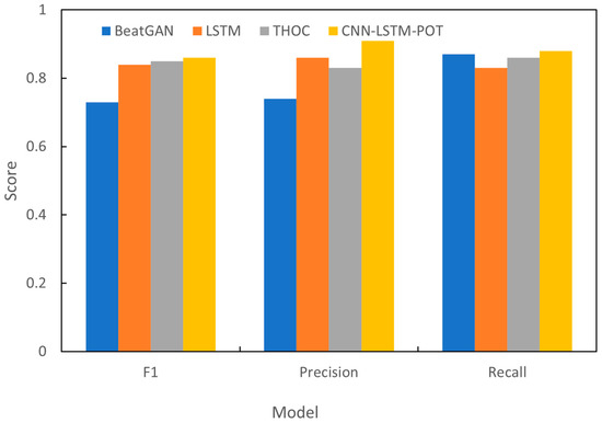
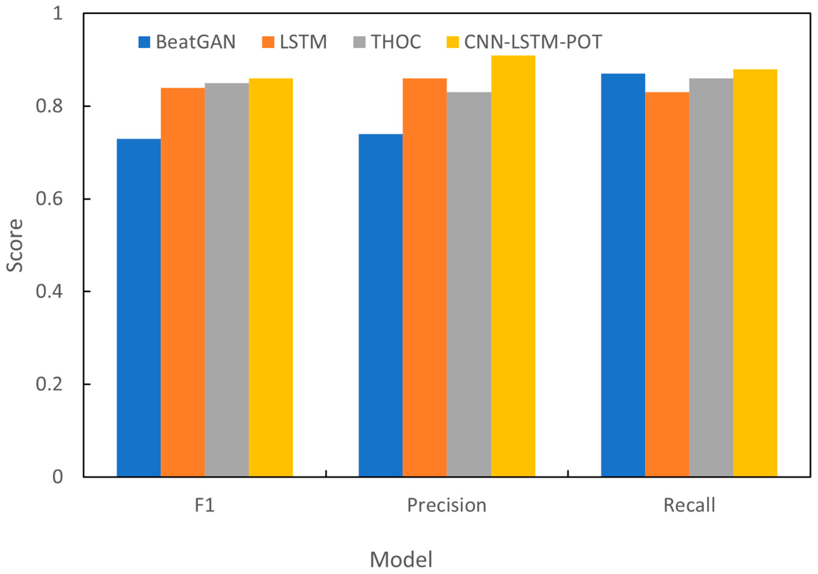
Figure 7 compares the performance of these four models using three evaluation metrics: Precision, Recall, and F1-score. The results indicate that the proposed CNN-LSTM-POT model outperforms the other methods across all metrics, demonstrating superior generalization and prediction capabilities in detecting anomalies.

Among the baselines, THOC achieves the second-best performance, reflecting its strength in modeling complex temporal patterns. In contrast, LSTM and BeatGAN perform relatively poorly, particularly in terms of F1-score and Precision. This may be attributed to LSTM’s limited capacity for extracting local features and BeatGAN’s susceptibility to mode collapse or training instability, especially when applied to large or complex datasets with high variability.

4.6. Edge Deployment Performance Analysis

To enable efficient deployment in resource-constrained edge devices, two optimization techniques were applied to the proposed CNN-LSTM-POT model to significantly improve operational efficiency while maintaining detection accuracy:

(1) Model Pruning

There exists a substantial number of redundant connections in the CNN-LSTM model, particularly within the weight matrices of fully connected layers and LSTM gating units, where many weight values approach zero and contribute negligibly to the final output. This paper adopts a magnitude-based pruning method. The model is first trained to convergence on normal data, after which the absolute value distribution of all weights is analyzed, and a global threshold of 0.01 is set. Weights with absolute values below this threshold are set to zero and subsequently skipped during inference. After pruning, the model assumes a sparse connection structure and is stored using the Compressed Row Storage format, reducing storage space occupancy. To further recover accuracy, the pruned model undergoes fine-tuning, allowing the remaining weights to adapt to the structural changes induced by pruning.

(2) Memory Pooling and Static Allocation

During edge device operation, frequent dynamic memory allocation and deallocation can lead to memory fragmentation, increased allocation latency, and potential memory insufficiency. Given the limited RAM resources of the STM32H743 (1 MB), memory usage must be strictly managed. This paper employs memory pooling technology. During the model loading phase, the input/output tensor dimensions and intermediate buffer requirements of each layer are pre-analyzed to calculate the maximum memory space required for the inference process. A fixed-size memory pool is then requested from the system at once. During inference, all tensors are statically allocated from this memory pool, and memory regions can be reused across layer computations (for example, the output space of a previous layer can be immediately allocated for use by the next layer after computation is complete).

Furthermore, a comprehensive comparison of all models was conducted on key edge deployment metrics, including memory usage, inference latency, and energy consumption. The detailed results are presented in

Table 5. Edge deployment performance comparison on the STM32H743 platform.

Metric	Model Size (KB)	Memory Usage (KB)	CPU Utilization (%)	Inference Latency (ms)	Energy Consumption (mJ)
CNN-LSTM-POT (Ours)	224.3	156.8	34.2	23.6	4.72
LSTM	128.6	102.4	21.5	15.2	3.04
BeatGAN	412.5	298.2	68.7	67.4	13.48
THOC	356.8	224.5	52.3	42.8	8.56

.

As shown in Table 5, the LSTM model achieves the lowest resource consumption across memory usage, inference latency, and energy consumption. The proposed CNN-LSTM-POT model achieves competitive performance across all metrics, while THOC and BeatGAN, due to their more complex architectures, demonstrate significantly higher resource consumption. Overall, the CNN-LSTM-POT model strikes a favorable balance between resource consumption and detection accuracy, and its moderate resource requirements enable it to meet the real-time edge deployment demands on the STM32H743 platform.

5. Application of the Algorithm in the Gateway

This study was conducted in a controlled greenhouse simulation environment, where a total of 40,320 data points were collected continuously over seven days from light intensity, temperature, humidity, and CO₂ sensors using an STM32F103C8T6 acquisition module (see

Table 6. Summary of collected sensor data and confirmed anomalies.

Sensor Type	Time Span	Total Data Points	Anomalous Data Count
Light Intensity (lux)	7 days	10,080	504
Temperature ($℃$)	7 days	10,080	412
Humidity (%RH)	7 days	10,080	379
CO2 (ppm)	7 days	10,080	473

for details). Anomalous data were generated through two approaches: natural sensor drift during normal operation and artificially introduced physical disturbances (e.g., suddenly increasing light intensity, igniting a flame). All anomalous data were labeled through manual verification, cross-validation with redundant sensors, and correlation analysis with environmental event logs. The dataset was chronologically divided into training (70%), validation (15%), and test (15%) sets to ensure the continuity of the time series and the fairness of evaluation.

5.1. Data Distribution Characteristics

To provide a comprehensive understanding of the collected dataset, we analyzed the distribution characteristics of each sensor type. Light intensity data exhibited a bimodal distribution, with peaks corresponding to daytime high-intensity periods (approximately 25,000–35,000 lux) and nighttime low-intensity periods (below 500 lux). Temperature readings followed a near-normal distribution centered at 24.5 °C, with a standard deviation of 3.2 °C, reflecting the greenhouse’s climate control system. Humidity data showed a right-skewed distribution, with values concentrated between 65% and 85% RH, occasionally dropping below 50% RH during ventilation events. CO₂ concentrations displayed a multimodal pattern, with baseline levels around 400–450 ppm and periodic elevations up to 800 ppm during plant respiration peaks.

5.2. Diurnal and Temporal Pattern Analysis

Significant diurnal patterns were observed across all sensor types, consistent with greenhouse environmental dynamics. Light intensity exhibited the most pronounced diurnal cycle, rising sharply after dawn (approximately 06:00) and peaking around noon (12:00–14:00), followed by a gradual decline after sunset (18:00). Temperature showed a correlated pattern with a 2–3 h lag behind light intensity, peaking in the mid-afternoon (14:00–16:00). Humidity displayed an inverse relationship with temperature, reaching maximum values during early morning hours (04:00–06:00) and minimum values during peak temperature periods. CO₂ concentrations exhibited dual peaks: a primary peak during nighttime (00:00–04:00) due to plant respiration, and a secondary peak during midday (12:00–14:00) potentially linked to reduced ventilation or human activity.

These temporal patterns were consistent across the seven-day collection period, with minor variations attributable to weather conditions (e.g., overcast days showing reduced light intensity and muted temperature fluctuations).

5.3. Anomaly Verification Methodology

All detected anomalous data were rigorously verified using multiple complementary methods to establish reliable ground truth. The verification process comprised the following approaches:

• Manual Verification: Domain experts visually inspected sensor readings alongside corresponding timestamps and environmental logs. For example, a sudden spike in temperature concurrent with a recorded ventilation system activation was classified as a normal event, whereas an unexplained temperature surge without corresponding actuator logs was flagged as a potential anomaly.
• Cross-Validation with Redundant Sensors: Each greenhouse node contained redundant sensors of the same type (e.g., two temperature sensors per node). Discrepancies between redundant sensors exceeding three standard deviations triggered further investigation. If one sensor deviated while its counterpart maintained expected readings, the deviating sensor was confirmed as anomalous.
• Correlation Analysis with Environmental Event Logs: The greenhouse control system maintained detailed logs of actuator events (e.g., ventilation activation, heating cycles, irrigation scheduling). Sensor readings were cross-referenced against these logs to verify whether observed deviations corresponded to legitimate control actions. For instance, a humidity increase following an irrigation event was classified as normal, while similar changes without corresponding logs were considered anomalous.

5.4. Experimental Scenarios and Gateway Performance

To assess the actual detection capability of the proposed CNN-LSTM-POT algorithm at the gateway level, four experimental scenarios were designed:

Experiment 1 (Single-sensor, single-node anomaly): A single sensor was perturbed—for example, by exposing a light sensor to strong illumination—to test the gateway’s response to isolated anomalies.

Experiment 2 (Multi-sensor, single-node anomaly): Multiple sensors within a single node were disturbed simultaneously (e.g., by applying fire near the node) to simulate correlated sensor failures.

Experiment 3 (Single-sensor, multi-node anomaly): The same type of sensor across multiple nodes was disturbed simultaneously (e.g., exposing multiple light sensors to bright light) to test detection performance under spatially distributed anomalies.

Experiment 4 (Multi-sensor, multi-node anomaly): Various types of sensors across multiple nodes were interfered with concurrently to simulate large-scale and heterogeneous abnormal scenarios.

Each experiment lasted 6 h, with a sampling interval of 3 min, and was repeated 50 times per scenario. In systems without the anomaly detection algorithm, all collected data were uploaded to the cloud. In contrast, the gateway with the integrated algorithm filtered out the anomalies locally, transmitting only clean data upstream.

By comparing the volume of transmitted data in both setups, the number of identified anomalies was inferred, allowing the calculation of the anomaly recognition rate (see Equation (16)). The results are shown in

Table 7. Gateway anomaly detection performance across experimental conditions.

Scenario Type	Total Data Points	Data Transmitted (with Algorithm)	Recognition Rate (%)
Single-node, single-sensor	120	74	92
Single-node, multi-sensor	120	82	76
Multi-node, single-sensor	120	77	86
Multi-node, multi-sensor	120	85	70

. All experiments were conducted in a controlled greenhouse simulation environment. Future work will involve deploying the system in operational greenhouses for extended validation.

These results demonstrate that the proposed algorithm is highly practical and adaptable for gateway deployments. It can significantly reduce the volume of anomalous data transmitted to the cloud, thereby relieving bandwidth consumption and computational pressure on cloud-based platforms. However, as can be seen from the table, the recognition rate decreases in the multi-node, multi-sensor experiment. The main reasons can be summarized as the following two points: correlations may exist among multi-sensor anomalies, and these correlations resemble normal environmental fluctuations, causing the model to misclassify correlated anomalies as normal variations, leading to missed detections; additionally, the multi-node, multi-sensor scenario presents the highest-dimensional feature space, where anomalies may simultaneously exhibit subtle deviations across multiple dimensions, increasing the difficulty for the model to distinguish between anomalies and normal patterns in this complex high-dimensional space.

6. Conclusions

This study presents a novel anomaly detection algorithm for greenhouse sensor data, integrating CNN, LSTM networks, and the POT method. The proposed CNN-LSTM-POT framework effectively combines the local spatial feature extraction capability of CNN, the temporal sequence modeling strength of LSTM, and the adaptive thresholding mechanism of POT based on extreme value theory. This integration enables accurate and efficient identification of anomalies in multi-source environmental data within greenhouse monitoring systems.

Specifically, the CNN component extracts multi-scale local features from raw sensor inputs, while the LSTM component captures temporal dependencies and evolving trends. The POT component then models the statistical distribution of reconstruction errors to derive adaptive thresholds and isolate anomalies. Working in concert, these three modules support both localized and system-level anomaly detection, improving the algorithm’s robustness and adaptability in noisy or variable greenhouse conditions.

Experiments demonstrate that the CNN-LSTM-POT model outperforms the baseline methods in detection accuracy, real-time throughput, and edge deployment suitability. The system substantially reduces the upload of erroneous data to the cloud, lowering both bandwidth consumption and server-side processing load. These results indicate that the proposed framework offers a practical, scalable, and dependable approach to anomaly monitoring in smart greenhouse applications, with clear potential for broader deployment in precision agriculture.

References

- Botta, A.; Cavallone, P.; Baglieri, L.; Colucci, G.; Tagliavini, L.; Quaglia, G. A Review of Robots, Perception, and Tasks in Precision Agriculture. Appl. Mech. 2022, 3, 830–854. [Google Scholar] [CrossRef] [Scilit]
- Pachouri, V.; Pandey, S.; Gehlot, A.; Negi, P.; Chhabra, G. Agriculture 4.0: Inculcation of Big Data and Internet of Things in Sustainable Farming. In 2023 IEEE International Conference on Contemporary Computing and Communications (InC4), Bangalore, India, 21–22 April 2023; IEEE: Bangalore, India, 2023; pp. 1–4. [Google Scholar]
- Ramankutty, N.; Mehrabi, Z.; Waha, K. Trends in Global Agricultural Land Use: Implications for Environmental Health and Food Security. Annu. Rev. Plant Biol. 2018, 69, 789–815. [Google Scholar] [CrossRef] [Scilit] [PubMed]
- Khan, N.; Ray, R.L.; Sargani, G.R.; Ihtisham, M.; Khayyam, M.; Ismail, S. Current progress and future prospects of agriculture technology: Gateway to sustainable agriculture. Sustainability 2021, 13, 4883. [Google Scholar] [CrossRef] [Scilit]
- Zhao, Y.; Gong, L.; Huang, Y.; Liu, C. A review of key techniques of vision-based control for harvesting robot. Comput. Electron. Agric. 2016, 127, 311–323. [Google Scholar] [CrossRef] [Scilit]
- Comparetti, A. Precision Agriculture: Past, Present and Future. In Proceedings of the International Scientific Conference “Agricultural Engineering and Environment—2011”, Akademija, Lithuania, 22–23 September 2011; pp. 1–17. [Google Scholar]
- Liang, L.; Qin, K.; Jiang, S.; Wang, X.; Shi, Y. Impact of epidemic-affected labor shortage on food safety: A Chinese scenario analysis using the CGE model. Foods 2021, 10, 2679. [Google Scholar] [CrossRef] [Scilit] [PubMed]
- Dhanaraju, M.; Ramalingam, K.; Pazhanivelan, S.; Kaliaperumal, R. Smart Farming: Internet of Things (IoT)-Based Sustainable Agriculture. Agriculture 2022, 12, 1745. [Google Scholar] [CrossRef] [Scilit]
- Hemming, J.; Edan, Y. Harvesting Robots for High-value Crops: State-of-the-art Review and Challenges Ahead. J. Field Robot. 2014, 31, 888–911. [Google Scholar] [CrossRef] [Scilit]
- Widyawati, D.K.; Ambarwari, A.; Wahyudi, A. Design and Prototype Development of Internet of Things for Greenhouse Monitoring System. In 2020 3rd International Seminar on Research of Information Technology and Intelligent Systems (ISRITI), 10–11 December 2020; IEEE: Yogyakarta, Indonesia, 2021; pp. 389–393. [Google Scholar]
- Jahnavi, V.S.; Ahamed, S.F. Smart Wireless Sensor Network for Automated Greenhouse. IETE J. Res. 2015, 61, 180–185. [Google Scholar] [CrossRef] [Scilit]
- Madruga Peláez, A.; Estevez Pérez, A.A.; López, R.S.; Santana Ching, I.; García Algora, C.M. Wireless Sensor Network in the Acquisition of Data in Greenhouses. Ingeniería 2019, 24, 224–234. [Google Scholar] [CrossRef] [Scilit]
- Pisanu, T.; Garau, S.; Ortu, P.; Schirru, L.; Macciò, C. Prototype of a Low-Cost Electronic Platform for Real Time Greenhouse Environment Monitoring: An Agriculture 4.0 Perspective. Electronics 2020, 9, 726. [Google Scholar] [CrossRef] [Scilit]
- Mohammadhossein Shekarian, S.; Aminian, M.; Mohammad Fallah, A.; Akbary Moghaddam, V. AI-powered sensor fault detection for cost-effective smart greenhouses. Comput. Electron. Agric. 2024, 224, 109198. [Google Scholar] [CrossRef] [Scilit]
- Aggarwal, C.C. Outlier Analysis; Springer: Cham, Switzerland, 2013. [Google Scholar]
- Zhaoxia, Z. Abnormal Data Detection Algorithm for Wireless Sensor Networks Based on PLC. In 2023 12th International Conference of Information and Communication Technology (ICTech), 14–16 April 2023; IEEE: Wuhan, China, 2023; pp. 521–525. [Google Scholar]
- Berjab, N.; Le, H.H.; Yu, C.-M.; Kuo, S.-Y.; Yokota, H. Abnormal-Node Detection Based on Spatio-Temporal and Multivariate-Attribute Correlation in Wireless Sensor Networks. In 2018 IEEE 16th Intl Conf on Dependable, Autonomic and Secure Computing, 16th Intl Conf on Pervasive Intelligence and Computing, 4th Intl Conf on Big Data Intelligence and Computing and Cyber Science and Technology Congress (DASC/PiCom/DataCom/CyberSciTech), 12–15 August 2018; IEEE: Athens, Greece, 2018; pp. 568–575. [Google Scholar]
- Kruthi, R.; Srivathsav, M.; Vinu Abinayaa, R.; Hemalatha, R. Clustering and Deep Learning—Based Anomaly detection in gas sensor data. In 2023 OITS International Conference on Information Technology (OCIT), 13–15 December 2023; IEEE: Raipur, India, 2024; pp. 190–195. [Google Scholar]
- Choi, Y.; Lim, H.; Choi, H.; Kim, I.-J. GAN-Based Anomaly Detection and Localization of Multivariate Time Series Data for Power Plant. In 2020 IEEE International Conference on Big Data and Smart Computing (BigComp), 19–22 February 2020; IEEE: Busan, Republic of Korea, 2020; pp. 71–74. [Google Scholar]
- Hashimoto, W.; Hirota, M.; Araki, T.; Yamamoto, Y.; Egi, M.; Hirate, M.; Maura, M.; Ishikawa, H. Detection of Car Abnormal Vibration using Machine Learning. In 2019 IEEE International Symposium on Multimedia (ISM), 9–11 December 2019; IEEE: San Diego, CA, USA, 2019; pp. 40–407. [Google Scholar]
- Hu, Z.; Chen, W.; Wang, H.; Tian, P.; Shen, D. Integrated data-driven framework for anomaly detection and early warning in water distribution system. J. Clean. Prod. 2022, 373, 133977. [Google Scholar] [CrossRef] [Scilit]
- Kwak, M.; Kim, S.B. Unsupervised Abnormal Sensor Signal Detection With Channelwise Reconstruction Errors. IEEE Access 2021, 9, 39995–40007. [Google Scholar] [CrossRef] [Scilit]
- Swate, C.; Sithungu, S.P.; Lebea, K. An Anomaly Detection Framework for IIoT in Agriculture. In Proceedings of the Ninth International Congress on Information and Communication Technology, Singapore, 25 July 2024; Springer: Singapore, 2024; pp. 419–429. [Google Scholar]
- Hinton, G.E.; Srivastava, N.; Krizhevsky, A. Improving neural networks by preventing co-adaptation of feature detectors. Comput. Sci. 2012, 3, 212–223. [Google Scholar]
- Goodfellow, I.; Bengio, Y.; Courville, A. Deep Learning; MIT Press: Cambridge, MA, USA, 2016. [Google Scholar]
- Song, J.C.; Zhang, L.Y.; Xue, G.X.; Ma, Y.P.; Gao, S. Predicting hourly heating load in a district heating system based on a hybrid CNN-LSTM model. Energy Build. 2021, 243, 110998. [Google Scholar] [CrossRef] [Scilit]
- Siffer, A.; Termier, A.; Largouet, C. Anomaly detection in streams with extreme value theory. In Proceedings of the 23rd ACM SIGKDD International Conference on Knowledge Discovery and Data Mining, Halifax, Canada, 13–17 August 2017; ACM: New York, NY, USA, 2017; pp. 1067–1075. [Google Scholar]
- Fawcett, T. An introduction to ROC analysis. Pattern Recognit. Lett. 2006, 27, 861–874. [Google Scholar] [CrossRef] [Scilit]
- Sak, H.; Vinyals, O.; Heigold, G.; Senior, A.; McDermott, E.; Monga, R. Sequence discriminative distributed training of long short-term memory recurrent neural networks. In INTERSPEECH 2014, Singapore, 14–18 September 2014; ISCA: Singapore, 2014; pp. 1209–1213. [Google Scholar]
- Zhou, B.; Liu, S.; Hooi, B.; Cheng, X.; Ye, J. BeatGAN: Anomalous rhythm detection using adversarially generated time series. In Proceedings of the 28th International Joint Conference on Artificial Intelligence, Macao, China, 10–16 August 2019; AAAI Press: Macao, China, 2019; pp. 4433–4439. [Google Scholar]
- Shen, L.; Li, Z.; Kwok, J.T. Time-series anomaly detection using temporal hierarchical one-class network. Adv. Neural Inf. Process. Syst. 2020, 33, 13016–13026. [Google Scholar]
Disclaimer/Publisher’s Note: The statements, opinions and data contained in all publications are solely those of the individual author(s) and contributor(s) and not of MDPI and/or the editor(s). MDPI and/or the editor(s) disclaim responsibility for any injury to people or property resulting from any ideas, methods, instructions or products referred to in the content. |
© 2026 by the authors. Licensee MDPI, Basel, Switzerland. This article is an open access article distributed under the terms and conditions of the Creative Commons Attribution (CC BY) license.