Article

Energy-Efficient Wireless Sensor Networks Through Coverage Hole Detection and Mitigation Using a Hybrid Raccoon–Hermit Crab Optimization Algorithm


by
Sean Laurel Rex Bashyam
and
Renuga Devi Subramanian
*
School of Electronics Engineering, Vellore Institute of Technology, Vellore 632014, India
*
Author to whom correspondence should be addressed.
Future Internet 2026, 18(3), 163; https://doi.org/10.3390/fi18030163
Submission received: 3 February 2026 / Revised: 10 March 2026 / Accepted: 16 March 2026 / Published: 19 March 2026

Abstract

Wireless sensor networks encounter issues like irregular deployment, node failures, and uneven energy consumption that create coverage holes, leading to a reduction in network lifetime in critical or disaster-based applications. Most existing approaches focus on coverage enhancement during the initial deployment and perform mitigation only at the beginning of the network operation. However, the coverage holes may also occur later due to node failures and energy depletion. To address this issue, a Hybrid Raccoon–Hermit crab optimization algorithm that advocates both initial coverage enhancement and adaptive mitigation due to future coverage holes is proposed. The proposed algorithm uses the global exploration ability of the raccoon optimization algorithm to find optimal cluster heads and the exploitation ability of the Hermit crab optimization to determine the optimal position and to relocate the static nodes logically to mitigate coverage holes. The proposed algorithm is evaluated under different node densities (50, 100, 200, 500, and 1000), with the sink at ( 100 , 100 ) . It results in an enhanced network lifetime of 65.20 % , an improved coverage ratio ( 16.94 % ) from ( 77.05 % ) to ( 93.94 % ) , increased throughput by delivering (3,139,293) bits, and a reduced delay of 2.27292 s for 1000 nodes compared with other existing methods.

Graphical Abstract

1. Introduction

Wireless sensor networks (WSNs) have become more essential in advanced disaster-related management systems, facilitating real-time monitoring, quick response to abnormalities, and efficient coordination during emergencies like avalanches, earthquakes, floods, forest fires, landslides, and tsunamis [1]. In such disaster scenarios, a large number of sensor nodes are deployed in target locations to continuously monitor changes in environmental parameters, detect abnormalities, and report or transmit priority data information to the base station (BS) or control center [2]. However, the functionalities of the WSNs were severely affected by limited battery capacity, a challenging and harsh deployment environment, and sudden node failures. Thus, providing energy efficiency and maximizing coverage remains a vital challenge for the sustainability of WSNs in disaster-related response systems.
As shown in Figure 1, traditional WSN follows a hierarchical architecture [2], where deployed sensor nodes (SNs) are grouped into smaller clusters, and each cluster is controlled or managed by cluster heads (CHs). These CHs collect data from the member nodes (MNs), aggregate the data, and forward it to the BS, thereby reducing redundant data transmissions and minimizing energy consumption. In particular, this architecture provides reliable data communication and adapts to scalability, which efficiently serves to offer wide area coverage and quick response in disaster-prone areas.
Despite this resilient architecture, WSNs face challenges such as high energy consumption. The nodes are battery-powered, and replacing batteries is often impractical. Moreover, they are deployed in irregular geographical locations, which reduces coverage. One of the most critical challenges in WSN is the formation of coverage holes [3], and they are broadly classified into two categories as:
  • Deployment-based coverage holes (coverage gaps): These occur due to uneven or random deployment, specifically in disaster-prone areas.
  • Failure-based coverage holes (future holes or black holes): Even if the network is well covered initially, new holes emerge as a result of continuous transmission over time in the network. Issues like node failures, energy holes (black holes), or physical destruction of nodes in disaster scenarios account for these types of coverage holes.
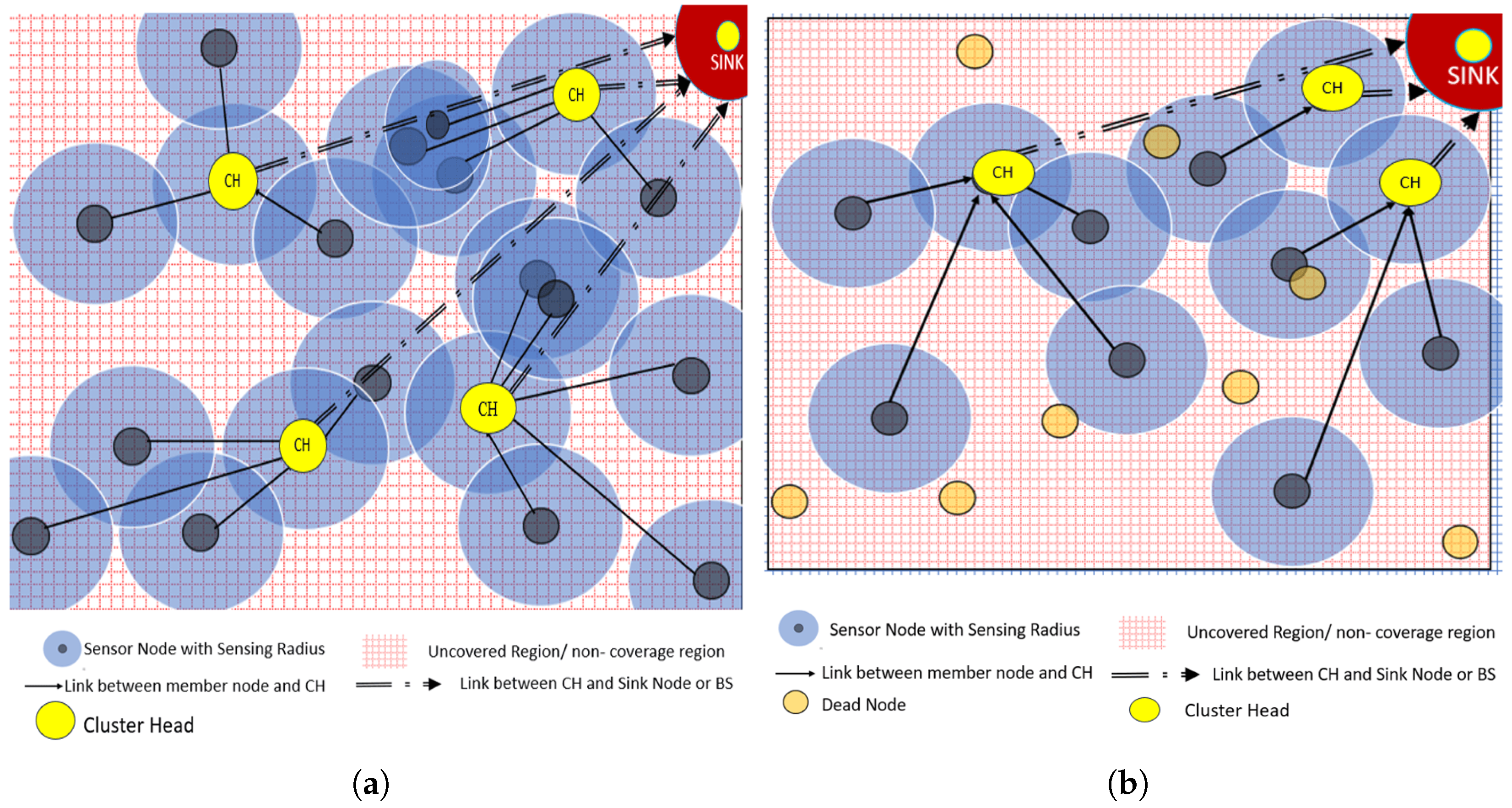
In disaster monitoring, the deployment-based coverage gaps and future failure-based coverage gaps are critical. Therefore, an effective WSN design must not only heal existing initial deployment holes but also adaptively respond to future holes arising from node failures to ensure reliability. From Figure 2, sensor nodes are deployed in the field, and each node is marked with its sensing range (circles around nodes in blue shade). The nodes in the network are grouped into smaller clusters. Member nodes (MNs) are connected to the cluster heads (CHs), and these MNs send data to the sink node through CHs. This approach is known as low-energy adaptive clustering hierarchy (LEACH) [4]. Conventional clustering protocols such as LEACH and its variants, including energy-aware LEACH (EA-LEACH) [5], distance-aware LEACH (DA-LEACH) [6], provide a baseline solution for energy-efficient communication. However, these protocols fail in disaster-based monitoring applications due to their inability to adapt dynamically to node failures, uneven energy consumption, and coverage imbalance.
To overcome these limitations, meta-heuristic algorithms have been introduced to improve optimized node deployment, enable efficient CH selection, detect coverage holes, and support hole healing under erratic and dynamically changing conditions. Nature-inspired meta-heuristic algorithms such as Genetic Algorithms (GAs) [7], Particle Swarm Optimization (PSO) [8], Fish Swarm Optimization (FSO) [9], Ant Colony Optimization (ACO) [10], Bat Optimization Algorithm (BOA) [11], have been widely used to address coverage holes. However, they exhibit limitations, including slow adaptation to rapidly changing environments, insufficient support for energy-aware solutions based on deployment conditions, and limited handling of multi-objective fitness functions involving coverage, computational overhead, energy, and distance. Additional challenges include poor handling of irregular shapes, difficulty adapting to newly added nodes, and trade-offs among parameter-sensitive constraints in real-time implementations.
To address these issues, a Hybrid Raccoon–Hermit Crab Optimization algorithm is proposed, integrating the Raccoon Optimization Algorithm (ROA) to balance exploration and avoid premature convergence and the Hermit Crab Optimization Algorithm (HCOA) for local parameter tuning to prevent suboptimal solutions and identify optimal node relocation for improved coverage. The method performs coverage hole detection and mitigation for both initial holes due to deployment and failure-based, emerging coverage gaps. In addition, HRHCOA not only maximizes coverage but also improves network performance metrics such as throughput, average delay, and energy consumption per round, which are essential in disaster-responsive applications and require faster detection in dire events, reliable data delivery, and extended network lifetime in both initial deployment-based coverage holes due to adverse environmental scenarios and failure-based future emerging coverage holes in each transmission round.
The major contributions of this work are as follows:
  • The proposed HRHCOA detects coverage holes around the network (exploration) and repositions nodes to optimal locations in each grid sector to heal the coverage holes (exploitation).
  • This proposed algorithm not only identifies and mitigates the initial deployment coverage holes but also mitigates the new coverage holes that emerge due to node failures during the network’s operation.
  • Simulation results indicate that the proposed algorithm has resulted in extended network lifetime, maximized coverage ratio, increased throughput, and lower delay when compared to LEACH and its variants, ROA and HCOA.
The rest of the paper is organized as follows: Section 2 offers insight into the various related works on coverage hole detection and healing techniques; Section 3 explains the problem formulation, network model, and assumptions taken into account for this work; Section 4 presents the proposed model and optimization technique in detail; Section 5 discusses the simulation setup and test outcomes; Section 7 examines the outcomes of the simulation scenario; Section 7 analyzes the performance metrics with comparative methods, spotlights key findings, limitations, and areas of improvement in the future; and finally, Section 8 concludes the work.

2. Literature Review

Recent technological advancements have paved out a way for WSNs to form a backbone of modern monitoring and control applications. This section coins the summary of recent contributions from 2010 to 2025 and relevant methods to overcome coverage holes in the network due to random deployment, irregular terrain, node failures, and energy depletion. Moreover, most of the existing works aim to reduce coverage holes emerged during the initial node deployment. Suitable solutions to overcome are discussed below and summarized in Table 1. Table 1 lists geometrical and LEACH-based approaches, Table 2 presents improvements based on initial meta-heuristic approaches, and Table 3 presents an advanced meta-heuristic approach to detect and heal coverage holes.
In [12], we proposed a Voronoi–Particle swarm optimization hybrid, emphasizing finding coverage and boundary for exact hole area calculation. It achieved coverage exceeding 95 percent, but incurred increased computational overhead in dense deployments. Similarly, ref. [13] has developed a gradient-based hole detection and repair method, which is quick in detecting holes but suffers from a suboptimal solution due to node relocation. Further, ref. [14] has used computational geometry for detecting boundary holes by evaluating detection accuracy and computational complexity, which led to high-accuracy boundary recognition and higher computational cost in large sensor networks. Reference [15], on the other hand, used a distributive detection collaborative protocol, which not only detected bounded or non-bounded coverage holes, but considered critical intersection points to find the hole. This approach reduces time complexity and helps in finding the holes in irregular terrain that are more common in practical WSNs.
Moreover, ref. [16] proposed mobile sensor scheduling to collect data in the specified path for optimal routing, which traces along the healed coverage zone, considering the path length and runtime to cover the dedicated network area, which marked a benchmark for mobile-based healing, but faces high computational complexity in large-scale networks. Moreover, this mobile node sensing is advanced by using a mobile robot-assisted precise healing method, which reduces repositioning time, improves accuracy, and heals the hole in a quicker time [17]. However, the complexity involved led to inefficiency in energy-based WSNs.
To overcome these limitations, a cluster-based energy-efficient protocol was proposed as LEACH [18], which grouped the WSN deployment into smaller clusters with each cluster group having a CHs and these CHs collect data from MNs and send it to the sink node or base station. This cluster-based method not only reduced energy consumption but also avoided early node death in the network, thereby postponing coverage holes caused by node failures. Furthermore, to overcome the constraints faced in LEACH, various improvements to the baseline LEACH are implemented in terms of energy, distance, load balancing, node mobility, and CH selection. These approaches are summarized in Table 1 below as follows.
Table 1. Comparison of coverage hole detection and healing techniques in WSNs.
ReferenceOptimization TechniqueKey ContributionsLimitationsStatic or Mobile
[19]Coverage Hole Optimization Protocol (CHOP)Balanced cluster head selection; approximately 20% coverage improvement over LEACHLacks proactive coverage hole prediction and healing mechanismsstatic
[20]I-LEACH with LeDiR-based healingDead node replacement using mobile sensors; extended network lifetime and improved connectivityRelocation delay and increased node overhead due to mobilitymobile
[21]DEAL protocol (distance- and energy-aware LEACH)Enhanced network stability and reduced probability of coverage hole formationHigher computational overhead during cluster head selectionstatic
[22]Delaunay triangulation-based detectionLow operational cost and scalable geometric hole detectionNo node relocation or healing strategy consideredstatic
[23]Adaptive probabilistic CH selectionReduced coverage hole formation and extended network lifetimeMisinterpretation of CH probability in certain operational roundsstatic
[24]Improved K-Means + enhanced LEACH with mobilityOptimized cluster head selection with mobile-node-based coverage hole healingRequires specialized coordination and control of mobile nodesmobile
Furthermore, to prolong the lifetime and maximize the coverage of WSNs, meta-heuristics optimization has been introduced to overcome the difficulties based on multi-objective functions. In particular, nature-inspired algorithms mimic the behavior of birds, animals, or any living organisms. These algorithms use the food searching or hunting nature to map with the WSN multi-objective function, such as CH selection, energy consumption from nodes, coverage maximization, and routing. In [25], a PSO-based optimization algorithm was designed to maximize coverage and improve energy efficiency in WSNs. The coverage range of each sensor is fixed, and the nodes are deployed in the field based on grids. The nodes inside each grid are under the control of a selected Grid CH. PSO is used to optimize the cluster group to select CH. This has shown an enhanced coverage ratio and reduced energy consumption. The main limitation of this model is that the network is static, homogeneous, not implemented in a real-time scenario and scalability for large scale networks.
Similarly, ref. [26] extended PSO to solve the k-coverage problem, ensuring that each target is covered by at least k nodes for improved reliability. This approach enhances fault tolerance, sensing accuracy, and balanced node utilization. However, it incurs high energy consumption due to redundancy and performs best in moderate-sized networks. This needs energy-aware K-coverage strategies and hybridization with clustering protocols. Similarly, ref. [27] evaluated multiple PSOs like inertia PSO, constriction PSO, and adaptive PSO for coverage optimization that improved convergence speed and candidate solution quality with the baseline PSO method. However, these methods show limited impact on broader WSN performance metrics, as they primarily focus on increasing coverage ratio while neglecting delay, fault tolerance, and real-time constraints. Furthermore, they do not meet multi- objective function such as delay, energy coverage, and inclusive improvement. To overcome these limitations, various requirements have been developed and adopted various other meta-heuristics methods to handle the energy and CH selection by fine-tuning the multi-objective constraints, which are listed in Table 2 as follows.
Table 2. Comparison of optimization-based coverage hole detection and healing techniques in WSNs.
ReferenceOptimization TechniqueKey ContributionsLimitationsStatic or Mobile
 [28]Hybrid PSO + VDCOAImproved connectivity, reduced coverage gaps, balanced energy in multi-hop networksAssumes stable clusters; ignores packet loss and delaystatic
[29]Genetic Algorithm (GA)Reliable multi-node k-coverage and improved fault toleranceHigh computational overhead in dense networksstatic
[30]GA-based cover set schedulingExtended lifetime and improved stability through coverage partitioningLimited QoS improvement; static homogeneous nodesstatic
[31]Hybrid GA (global + local search)High coverage and QoS stability across varying node densitiesHigh delay and uneven energy usage under dynamic conditionsstatic
[32]Adaptive GA variantsEnergy-efficient coverage maximizationSimulation-only; static deploymentstatic
[33]Improved dynamic GA deploymentMaximized coverage with reduced redundancyDeterministic model; lacks probabilistic QoS analysisstatic
[34]GA + ACO hybridReduced early hole formation and optimized CH–BS routingHigh complexity in dense networksstatic
[35]ACO + hill climbingEnergy-aware node activation and improved coverageLocal optimization bias in sparse networksstatic
However, initial meta-heuristics methods were able to avoid or reduce constraints, such as slower convergence, sub-optimal traps, and erratic behavior. As deployment complexity increased, more advanced metaheuristic techniques were introduced to address emerging multi-objective constraints, as summarized in Table 3 as follows.
Table 3. Comparison of advanced meta-heuristics optimization techniques to heal coverage holes.
ReferenceOptimization TechniqueKey ContributionsLimitationsStatic or Mobile
 [36]Grey Wolf Optimizer (GWO)Optimized node spacing and reduced coverage holesLimited to static deploymentsstatic
[37]Hybrid GWO (Levy + RL)Superior coverage improvement over PSO and GANot suitable for dynamic environmentsstatic
[38]Weighted GWO + DT + RSSILow latency, high throughput in disaster-prone WSNsMobile node coordination complexitymobile
[39]Whale Optimization Algorithm (WOA)Achieved ∼90% coverage and stabilitySensitive to uneven node distributionstatic
[40]COOT Bird OptimizationImproved coverage in uneven deploymentsNo mobility or QoS modelingstatic
[41]WHO + Golden SineReduced redundancy in obstacle environmentsIncreased algorithmic complexitymobile
[42]Jellyfish Algorithm + LEACHAchieved ∼85% coverage with mobile sensorsUnstable in sparse networksmobile
[43]BAT AlgorithmEnergy-efficient CH selection and coverage stabilityProne to local optimastatic
[44]HGWO–PSO/HGWO–HSAImproved robustness, coverage, and trap avoidanceHigher computational overheadstatic
For multi-objective clustering strategies, such as optimal CH selection, proper load balancing and distribution, a raccoon optimization algorithm (ROA) was proposed based on its prey-search and den-acquiring behavior. It demonstrated significant improvements in energy efficiency, QoS metrics, stability, and network lifetime [45]. Its faster convergence and ability to overcome sub-optimal traps show its stable behavior and make it suitable for maximizing coverage. By segregating clusters based on fitness function, it improves the traditional cluster formation process and CH selection, allowing CHs to choose their own MNs. This enhances stability, reduces intra-cluster distance, and achieves performance comparable to baseline LEACH, while providing higher throughput, lower delay, and more stable operation.
In [46], a novel hermit crab optimization (HCO) method aims to address coverage holes formed due to initial deployment, which were not in transmission range, and it optimizes nodes to move into new locations. Here, delauny triangulation and RSSI-based localization are performed for determining whether the node is in transmission range or not for its nearby neighbor. Whenever a hole or isolated node is detected, HCO finds an optimal location to reposition the isolated node and repairs the network based on its strong exploration and exploitation capability, avoiding premature convergence, staying stable, and improving search optimization compared to PSO and GWO. This is validated using the F-1 score to optimize fitness evaluation by considering energy, coverage, routing path, and delay. This algorithm focused on both non-coverage regions and isolated nodes, where isolated node repositioning was not considered in previous works.
In summary, traditional protocols and cluster-based approaches, along with multi-objective metaheuristic bio-inspired methods, have been employed in WSNs to improve energy efficiency, optimize CH selection, enhance node connectivity, and maximize coverage. Building on this, the proposed Hybrid Raccoon–Hermit crab optimization algorithm uses raccoons’ global search (exploration) for optimal CH selection and hermit crabs’ local refinement (exploitation) to reposition nodes closer to uncovered areas within each grid sector. This approach improves energy efficiency, extends the network’s lifetime by maximizing coverage, and addresses both initial deployment-based holes and emerging holes caused by node failures or isolated nodes without leveraging the QoS metrics.

3. Network Modeling

This section considers a suitable radio model that accounts for both node energy consumption and the repositioning mechanism. It also reviews standard cluster formation and CH selection techniques and their variants, as well as enhanced bio-inspired methods that serve as a baseline for the proposed model.

3.1. First-Order Radio Model (Energy-Based)

3.1.1. Basic First-Order Radio Model

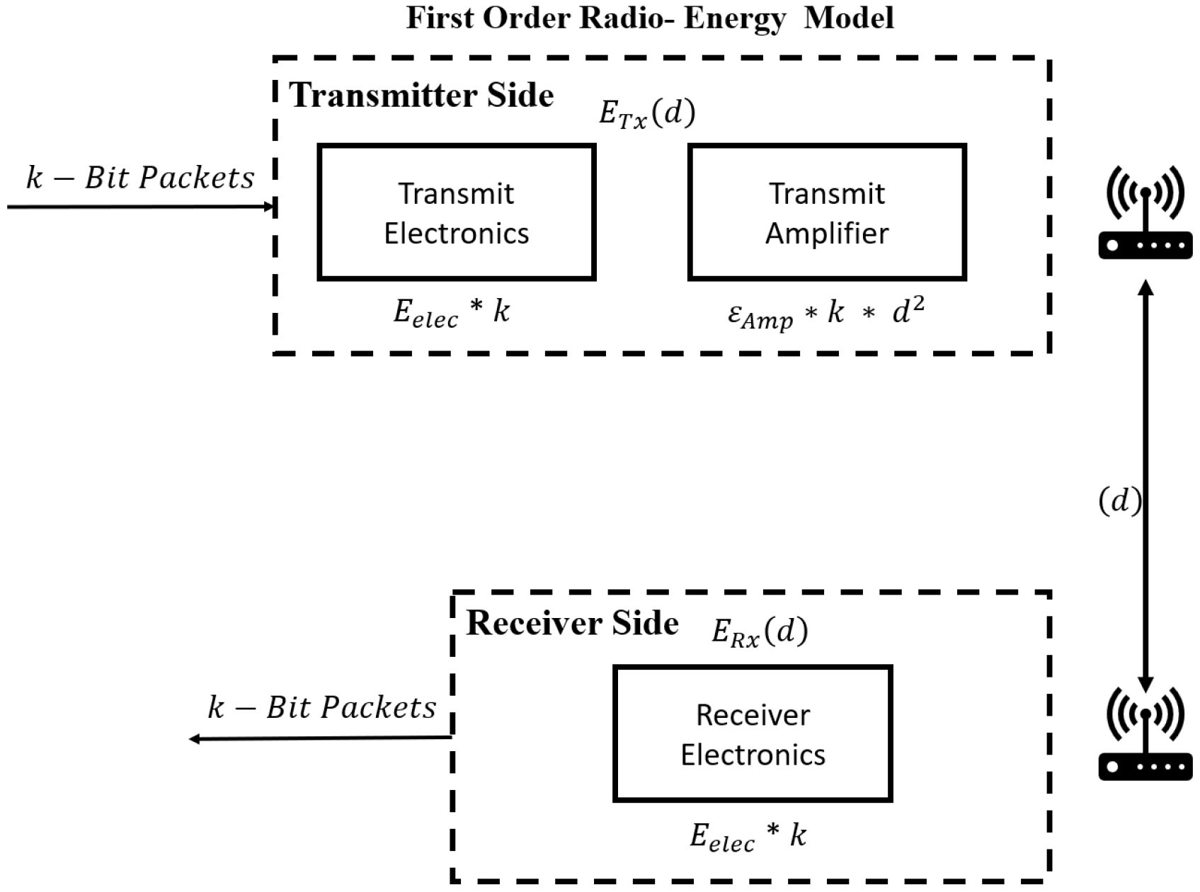
A WSN typically performs sensing, data processing, data transmitting, and receiving, where transmitting and receiving are complex, energy-consuming processes. Therefore, choosing an appropriate energy model for physical deployment helps to form an efficient WSN [18]. A SN acts as both a transmitter and a receiver. Accordingly, the following radio model is formulated, as shown in Figure 3. The total energy consumed by an SN to transmit ( E t x ) and receive ( E r x ) a k-bit message over a distance d depends on the characteristics of the wireless channel and is defined by the following equations.
Energy consumed on the transmitter side as in Equation (1) as,
E tx ( k , d ) = E elec · k + ϵ amp · k · d 0 n
where
  • E elec : Energy consumed per bit for electronics.
  • ϵ amp : Energy consumed by the amplifier.
  • k: Number of bits in the packet.
  • d: Distance between transmitter and receiver.
  • n: Path-loss exponent (typically 2 or 4).
  • d 0 : Threshold distance (propagation model).
The threshold distance that determines the propagation model is given in Equation (2),
d 0 = ϵ fs ϵ mp
where
  • ϵ fs : Energy consumed by amplifier in free space model.
  • ϵ mp : Energy consumed by amplifier in multi path.
The energy consumed at the receiver side is given by Equation (3):
E rx ( k ) = E elec ( k , d ) + E rx ( k )
And total energy consumed can be calculated as in Equation (4):
E T = E tx · k + ϵ amp · k · d 0 n

3.1.2. Node Repositioning Radio Model

This work focuses on improving coverage by relocating nodes to optimal positions. This process consumes energy for node relocation as well as for data transmission and reception in each round after relocation.
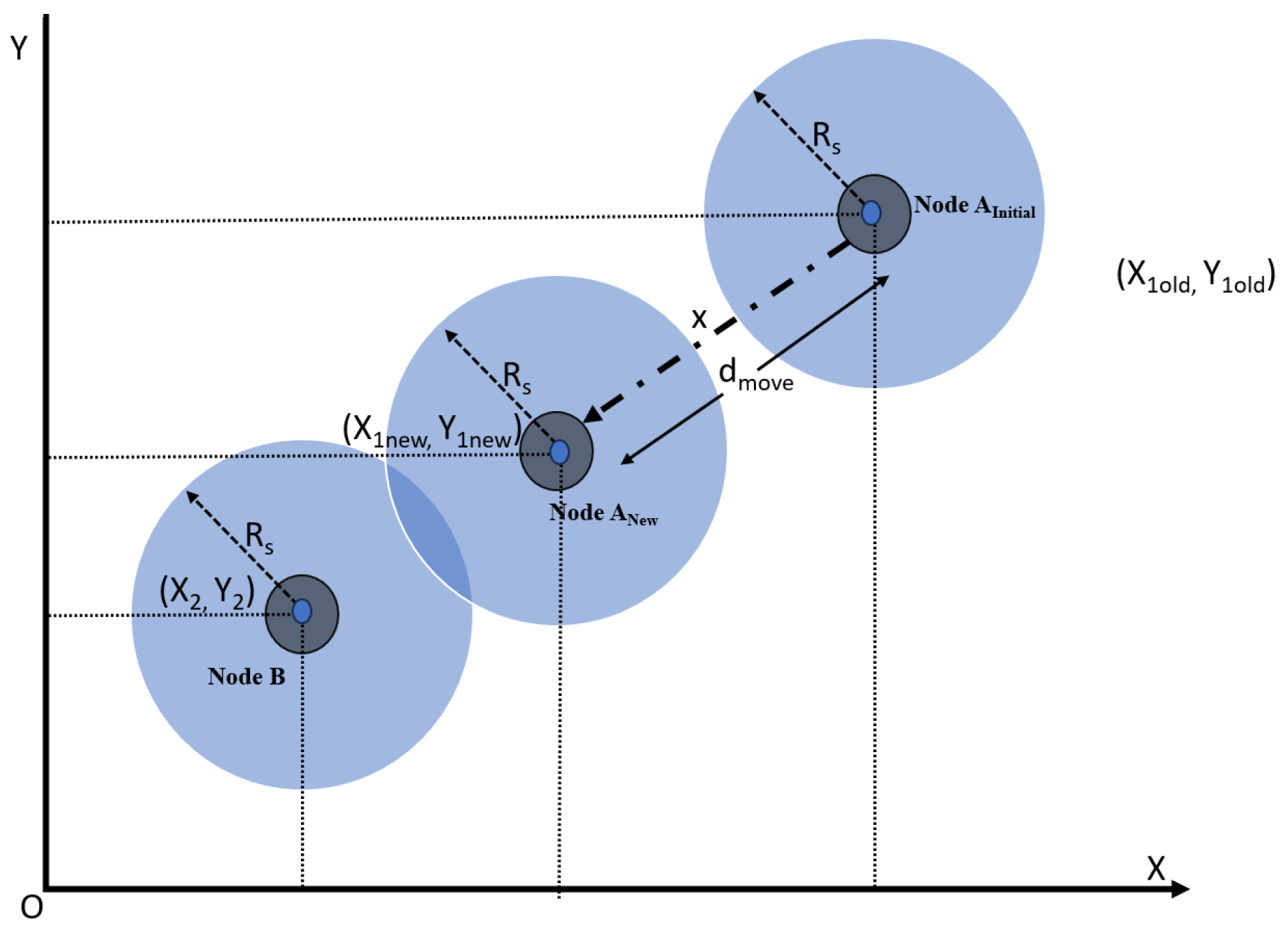
As shown in Figure 4, the distance moved by a node along a linear path is given in Equation (5):
E move ( d move ) = E move-per-m · k
where
  • E move-per-m : Energy consumed per bit by mobility platform J / m
The acceleration energy required for moving the node to a new position is in Equation (6):
E move = 1 2 m v 2 + C · d move
The linear energy model is simpler to compute energy consumption and can be expressed as Equation (7):
E total = E move ( d move ) + E tx ( k , d new ) + E rx ( k )
Additionally, let us assume and consider if node A wants to reposition nearby and transmit data to node B in an energy-aware and distance-limited scenario as follows:
  • They are currently disconnected and separated: d > d 0 ;
  • Assume, node A has enough energy to reposition and perform communication in Equation (8);
    E res ( A ) E move ( d req ) + E tx ( k , d new )
    where
    • E res : Safety margin of residual energy between (10–20%).
    • d req : Required movement distance and should be strictly under the distance threshold.
  • To limit excessive node relocations, the required movement distance and mobility budget threshold ( D th ) are determined based on the sensor’s sensing range and a scaling factor α ranging from 0.5 to 1, as defined in Equation (9).
d req D th
The required distance to reposition to a smallest distance s from ( d ) ( d req ) is determined and should satisfy d req d max and is denoted in Equation (10):
d req = max ( 0 , d d max )
where
  • d req : Required movement distance and should be strictly under the distance threshold.
  • d new : New distance to the node to move.
  • d max : Maximum distance the node is moved.

3.2. Low-Energy Adaptive Clustering Hierarchy (LEACH) Protocol and Its Variants

LEACH protocol is a hierarchy-based protocol [4], which divides the total group into smaller clusters and each cluster is controlled by CHs to collect data from MNs, the data from MNs were aggregated, and priority data is forwarded to BS. Here, stochastic algorithms were used to determine which node to select from its cluster group, and these were decided based on the highest energy left in the node, which has the shortest distance between CH and BS for each round.
The leach protocol assumes the following:
  • All nodes are randomly deployed and static.
  • All nodes have the same initial energy, sensing, and communication range.
  • BS is placed at the far end of the network, and it is immobile.
The probability of a member node being selected as CH is denoted as in Equation (11):
P ( i ) = p 1 p r mod 1 p , if i G , 0 , otherwise .
where
  • P: Desired CH probability.
  • r: Current round.
  • 1/p: Number of rounds in one epoch or iteration.
  • G: Set of nodes that has not been selected as CH in previous (1/p) rounds.
The total energy dissipated in a cluster group, considering the first-order energy model for transmitting and receiving data, can be expressed as in Equation (12):
E cluster = n · k · E elec + k · ϵ f s · d C H 2 + ( n 1 ) · k · ϵ f s · d member 2
where
  • E cluster : Energy consumed by the cluster.
  • n: Number of nodes in the cluster.
  • d CH : Distance from CH to BS.
  • d member : Average distance between member nodes and CH.
The residual or energy left in the node is formulated as in Equation (13):
E residual = E initial ( E tx + E rx )
Furthermore, coverage-based LEACH repositioning in terms of energy spent to move a node or CH to a new location is expressed as in Equation (14):
C eff = C 0 α · E move
where
  • C eff : Effective coverage after repositioning.
  • C 0 : Initial coverage (before repositioning).
  • E move : Energy spent to move a node or CH.
  • α : Weight factor: A parameter that characterizes the rate at which coverage decreases with increasing energy consumption.
The coverage in terms of energy required for node relocation, constrained by a threshold to limit resource overuse, is expressed in Equation (15):
C eff = 1 A A 1 i = 1 N 1 1 { d i ( x ) R s , E i > E th } d x
where
  • E i : Residual energy of the node i.
  • E th : Threshold energy, where a node cannot move.
  • d i ( x ) : Distance from point of x to node.
  • R s : Sensing range of a node.
Even though the LEACH improves energy consumption of the network, its frequent CH rotation drains the CH energy faster. To enhance the LEACH protocol, several modified variants have been proposed, including threshold energy-based LEACH ( I L E A C H E A ) [5], threshold distance-based CH selection using deterministic LEACH ( I L E A C H D A D ) , and probabilistic LEACH ( I L E A C H D A P ) [6].
The effective coverage of I-LEACH-EA is termed as in Equation (16):
C eff = 1 A E A E n i = 1 N 1 1 { d i ( x ) R s , E i > E th } d x
where
  • AE: Overall Sensing area with respect to the energy model.
  • N: Number of high-energy nodes.
Similarly, for distance based I L E A C H D A , the effective coverage after distance aware deterministic method is in Equation (17):
C eff = 1 A D D A D D n i = 1 N 1 1 { d i ( x ) R s , E i > E th } d x
  • A D D : CH threshold selected based on deterministic distance between CH and BS.
The effective coverage of probabilistic-based selecting CH with distance function is in Equation (18) as:
C eff = 1 A E P A E P n i = 1 N 1 1 { d i ( x ) R s , i active } d x
  • A D P : CH threshold selected based on probabilistic distance between CH and BS.

3.3. Raccoon Optimization Algorithm

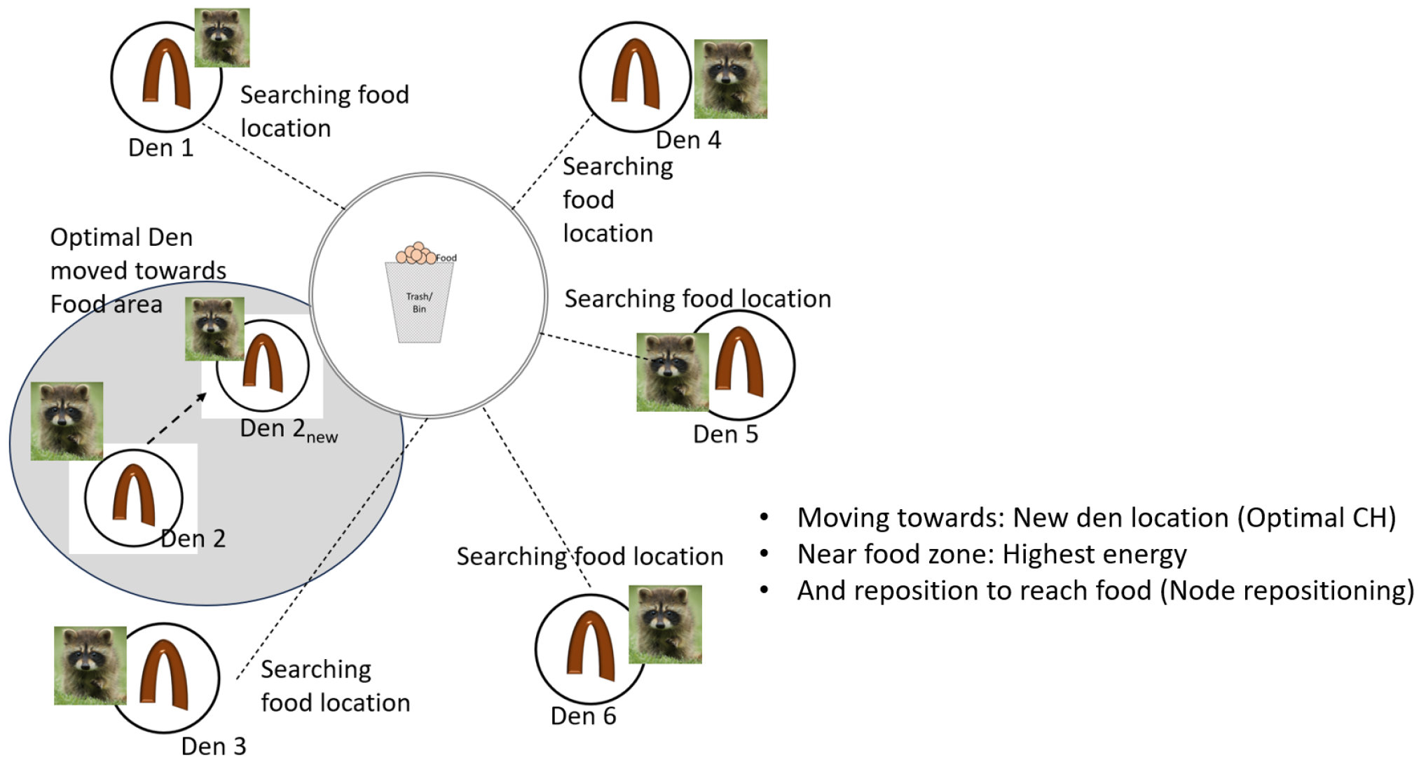
As shown in Figure 5, the Raccoon optimization algorithm (ROA) [45] is based on raccoons’ foraging and food search behavior that uses its sensory intelligence to select the best food locations in a wide area and relocates it den closer to the food’s location. In a random space, a set of raccoon populations is initialized for its food search process, and each candidate represents a potential solution (e.g., node positions or cluster head selection). Further, the raccoon explores the environment by moving towards the unattended area and ensures global search and avoids local optima. Similarly, with the help of the best local solution, it repositions its location and updates it to improve coverage, energy efficiency, and connectivity. This search process is repeated until convergence rules are met, and the best local solution is used to fairly select the finalized optimized result as a potential solution.
Maximum coverage of all the nodes in the network is expressed as in Equation (19):
C ( x , y ) = 1 i = 1 N 1 C i ( x , y )
Once the holes are found in the deployment, ROA is employed to heal the holes formed.
Let us initialize the ROA population solution p i in the region and update the P f i t n e s s value as in Equation (20):
p i ( t + 1 ) = p i ( t ) + w Δ p i explore + ( 1 w ) Δ p i exploit
In the exploration phase, the global search parameter is determined as in Equation (21):
Δ p i explore = α · ( p h p i ( t ) ) + β r 1
In the exploitation phase, the local tuning parameter is defined in Equation (22):
Δ p i exploit = γ · ( p best p i ( t ) ) + δ · r 2
where
  • α : Exploration weight, moving towards the guiding point p h .
  • β : Random exploration factor to avoid local optima.
  • γ : Exploitation weight for moving towards best-known position p b e s t .
  • δ : Random exploitation factor to avoid stagnation.
Further, ROA finds an optimized node (neighboring-node) to move towards the hole’s location to fill the gap. The position update is defined in Equation (23) and the corresponding fitness function is given in Equation (24):
p i ( t + 1 ) = p i ( t ) + λ p h j p i ( t )
F i = ( x , y ) H i 1 η · i E move ( Δ p i )
where
  • p i ( t ) : Current position of node i at time t.
  • p h j : Guiding point from helper/neighbor node j.

3.4. Hermit Crab Optimization Algorithm

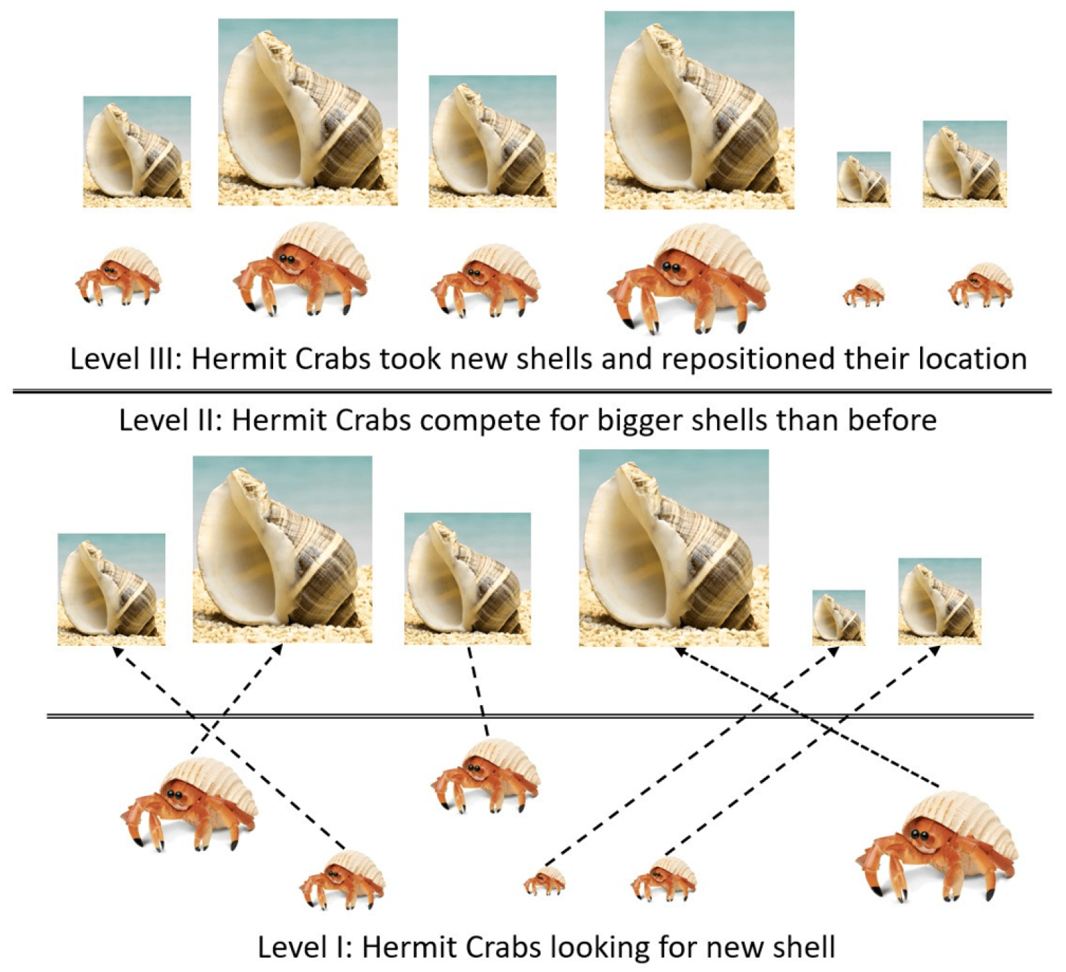
As shown in Figure 6, the HCO mimics the natural behavior of Hermit Crabs (HCs) to find the best shells. These HCs do not grow their own shells; instead, they often seek the largest shells to hide out for their protection through a process known as exchange or migration, and this process is repeated until the best shell is found and continued till death. The candidate solution (crabs) tries to find resources or solution space (shells) using their global search or exploration for possible solutions and computes or exchanges for the best shells (exploitation for optimal results). It balances HCO to avoid local optima and move towards the global best solution, as it is simple, flexible, and efficient in solving complex combinatorial optimization problems. Here, HCO aims to address two main issues in WSN: optimal CH selection and finding coverage holes to heal for maximizing coverage. Inspired by HCs’ shell-seeking behavior, the algorithm is modeled accordingly [46].
By employing HCO’s exploration and exploitation phase, holes are healed under the following condition E i > E t h to move the node towards the best local coverage (shells), and the position is updated as in Equation (25):
p i ( t + 1 ) = p i ( t ) + s 1 p b e s t p i ( t ) + s 2 r
where
  • p b e s t : Best local coverage position (shell).
  • r: Random vector for exploration.
  • s 1 , s 2 : Control parameters for exploitation and exploration.
Energy-aware movement can be traced as in Equation (26):
E i ( t + 1 ) = E i ( t ) k p i ( t + 1 ) p i ( t ) 2 E t x
The fitness function is evaluated as in Equation (27):
F i = ( x , y ) H i 1 λ · E move ( p i )
The neighboring nodes move towards to heal the gap and the new position (exploitation) is updated p i ( t + 1 ) as in Equation (28):
p i ( t + 1 ) = p i ( t ) + γ p h j p i ( t ) + η p r p i ( t )
where
  • γ : Exploitation weight (toward the hole).
  • η : Exploration weight (random movement).
  • p r : Random position in the sensing field.
Individually, ROA and HCO confronts few limitations in cluster-based WSN. ROA performs better and ensures globally optimized CH selection and repositions it to the best position, but uneven distribution and its limited knowledge on local search do not fully support healing holes effectively. Whereas, HCO offers better and optimized repositioning to nodes, but limits global energy-aware CH selection, which leads to premature node death as energy depletes unpredictably and unbalanced clustering.

4. Proposed Method: Hybrid Raccoon-Hermit Crab Optimization (HRHCOA)

In order to extend the network lifetime, efficient clustering, minimized energy consumption, balanced node distribution, and maximized coverage are crucial. This work focuses on proposing a hybrid framework that combines ROA [45] and HCO [46] as the Hybrid Raccoon–Hermit Crab Optimization Algorithm (HRHCOA) that enhances efficient coverage by minimizing holes and extending the network lifetime in LEACH-based clustering WSNs.
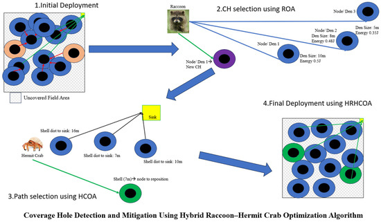
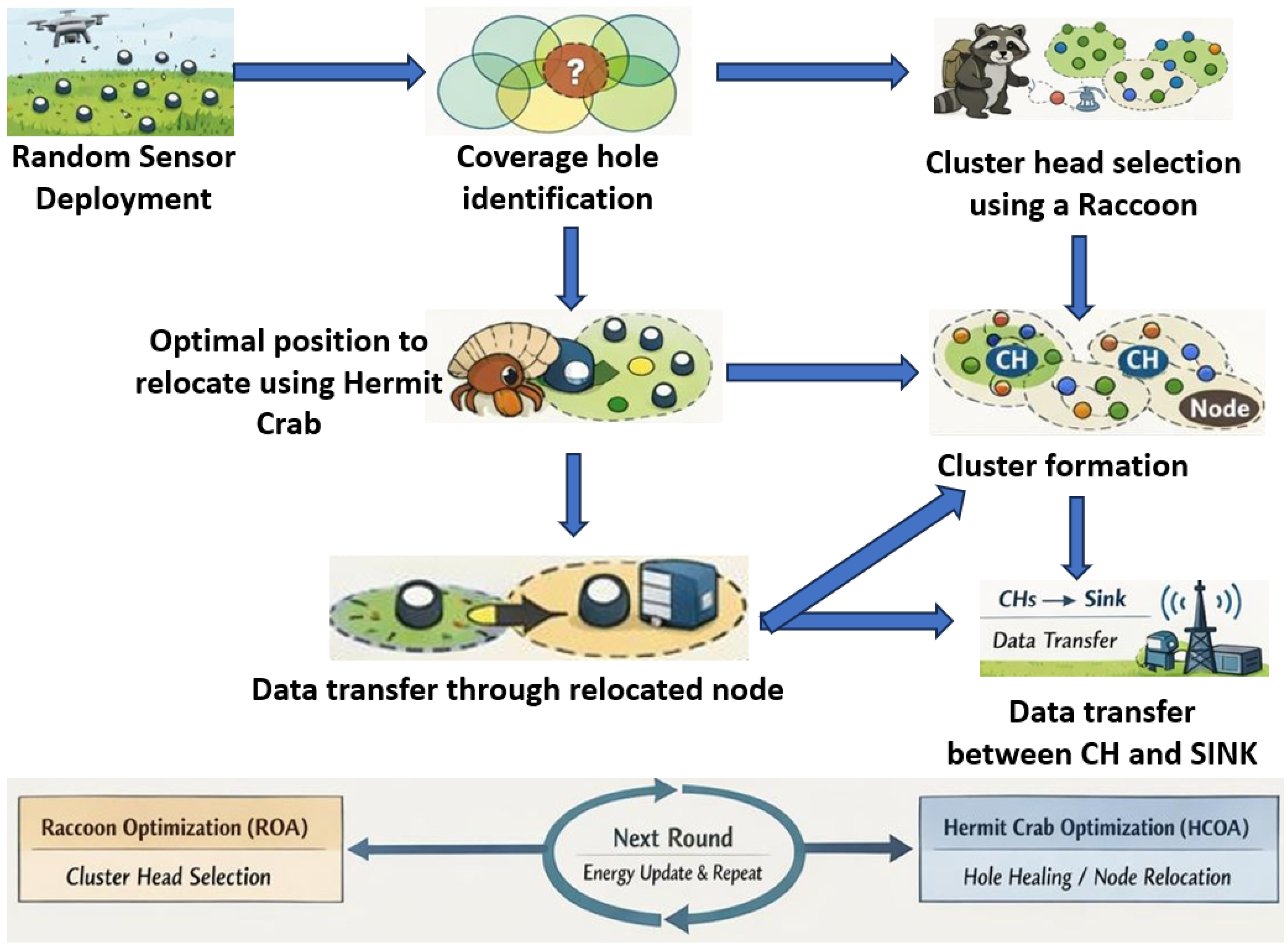
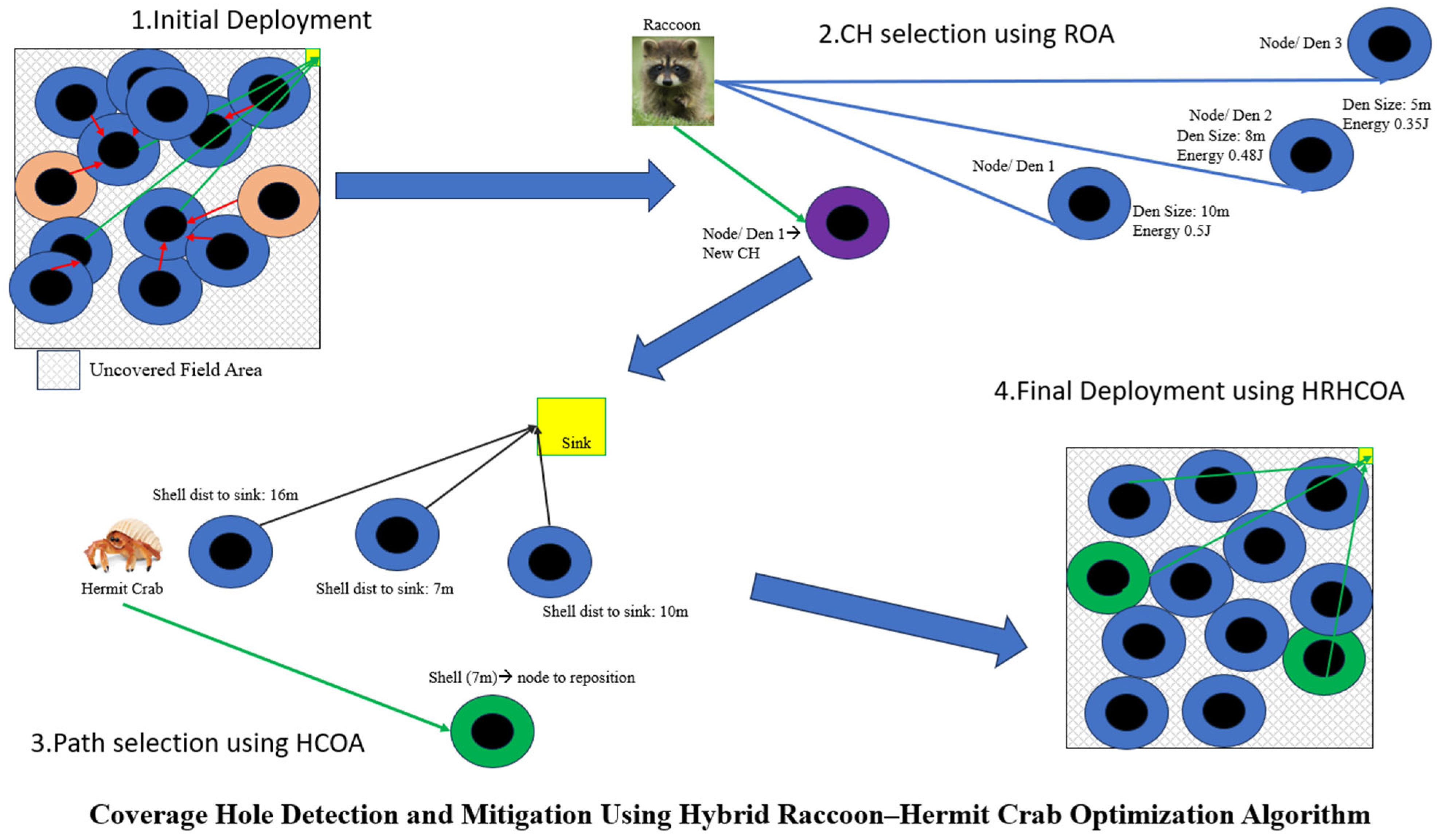
As shown in Figure 7, a group of sensor nodes is randomly deployed in the sensing field area to monitor for any activity. Once the sensor nodes are deployed, they connect together to form a network using the sensor nodes’ sensing range R s , and during such network formation, a few nodes may not be a part of the cluster formed due to their spatial deployment, irregular node deployment, and geographical irregularities. This leaves some areas unattended and creates coverage holes. Once these holes are identified, our proposed HRHCOA uses ROA’s den sharing ability to choose an optimal CH and identify the left-out MNs to connect them back to the network to re-cluster. Even after re-clustering, some nodes may not be able to join the network, and HRHCOA uses HCOA’s shell-finding ability to identify the new position in order to enable the sensor node to join the existing cluster. Once a new cluster is formed, the MNs transfer data to the sink node through the newly elected CHs.

4.1. Network Modeling

Let us assume the following to design a network model to detect and mitigate coverage holes in the network. A first-order mobility based radio model is considered for modeling with sensing radius R s and communication radius R c , energy parameters like E t x , E r x , energy for the node i at round t as E i ( t ) , energy for node to move as E m o v e ( Δ p ) = k . Δ p 2 , and energy threshold E t h .

4.1.1. Initial Deployment and Hole Healing

The node coverage at vector position P i is indicated in Equation (29):
C i ( x , y ) = 1 , if ( x , y ) p i   R s 0 , otherwise
and total coverage in the network is expressed as in Equation (30):
C ( x , y ) = max i C i ( x , y )
The coverage holes arising from initial deployment in uncovered regions are defined in Equation (31) as:
H init = ( x , y ) A 1 C ( x , y )
where the detected hole cluster H j and its centroid [ P h j ] are defined in Equation (32):
p h j = 1 | H j | ( x , y ) H j ( x , y )

4.1.2. ROA-Based Global Search

Each raccoon stands up for a candidate solution i s CH configuration, and the fitness function is expressed as in Equation (33):
F i = w 1 E res E avg + w 2 1 d B S w 3 H init A h
where
  • E r e s : Residual energy.
  • E a v g : Average energy.
  • d B S : distance to base station.
  • A h : total healed area.
With the help of the fitness function, an optimal CH is selected, and the position of the new CH node is updated as in Equation (34):
p i ( t + 1 ) = p i ( t ) + γ p best p i ( t ) + η rand p neighbor p i ( t )

4.1.3. HCO-Based Local Tuning

After finding the hole centroids P h j , the nodes that are found to be optimal are repositioned using HCO’s local tuning function, and the new position of node i is updated as in Equation (35):
p i ( t + 1 ) = p i ( t ) + λ p h j p i ( t ) + δ rand ( )
where
  • λ : Directed movement of node towards the hole centroid.
  • δ : Adaptive random shift using crabs behavior.

4.1.4. Healing Performance

The performance effectiveness of healing in each round t for repositioning node i is defined in Equation (36):
H i heal = C old ( A h ) C new ( A h )
where
  • A h : Affected hole area (number of grids oints).
  • C o l d a n d C n e w : Coverage before and after healing calculated based on points in each grid sector.
The final coverage after HCO local refinement can be expressed as in Equation (37):
C final = A H initial A
If C final = 1 , this indicates complete restoration; if C final < 1 , coverage holes remain in the network.

4.2. HRHCOA Algorithm and Flowchart

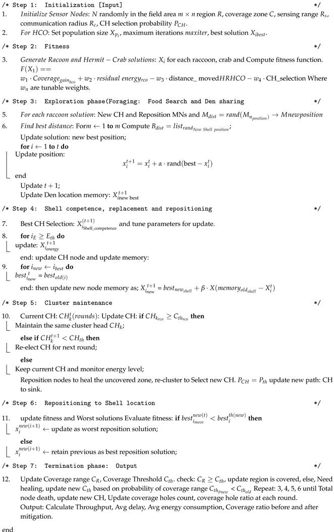
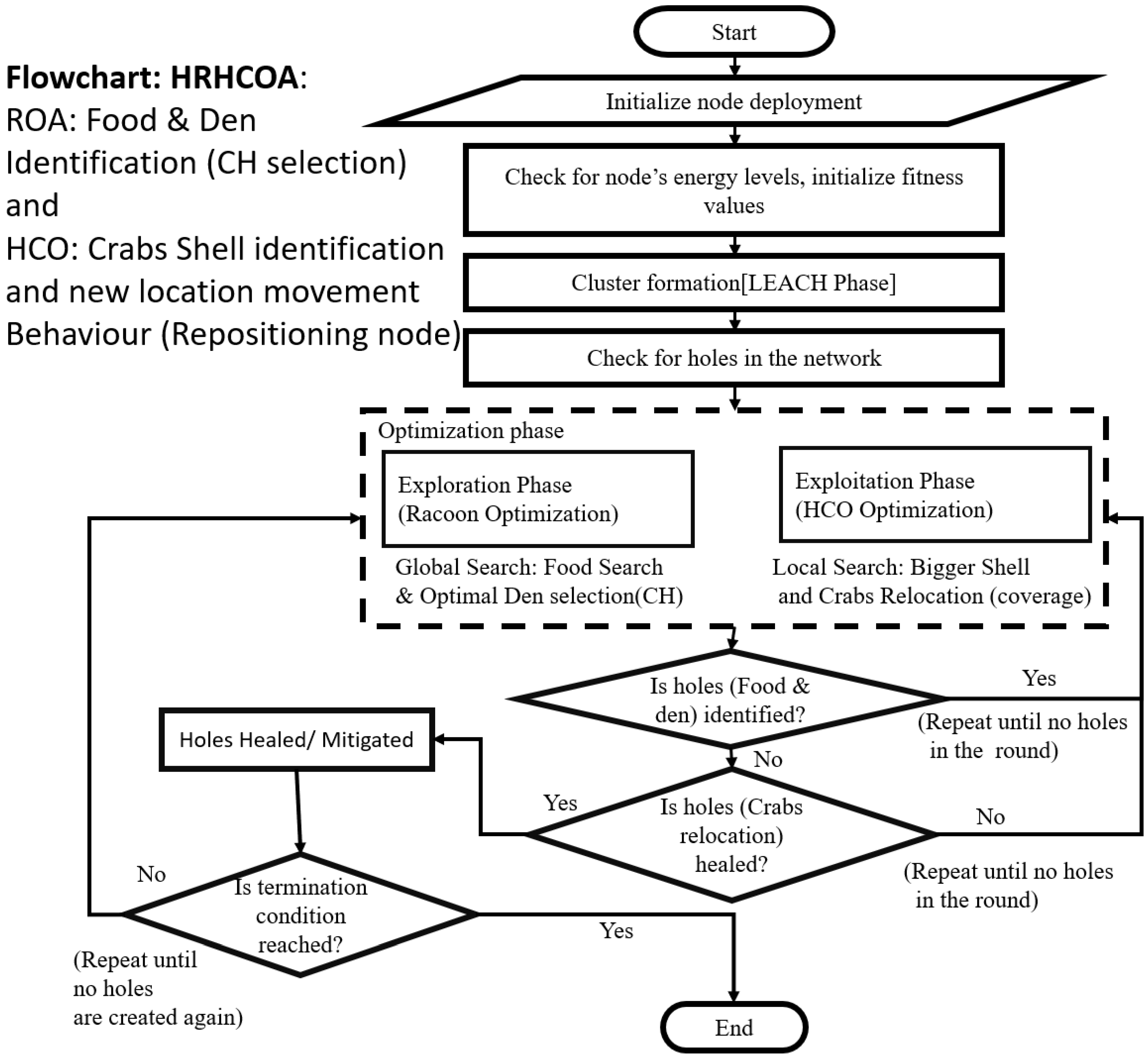
As shown in Figure 8 and Algorithm 1, once the nodes are randomly deployed in the network, the LEACH is responsible for cluster formation and CH selection using energy and distance parameters. Furthermore, the network is checked for coverage holes. If no hole is found, then the data transmission operation begins; if holes are found, the network prepares for the hole detection and repair process using our proposed HRHCOA algorithm. With ROA’s global search ability, the nodes with the highest energy are selected as CH. This forms a new cluster group, and this may help to reduce holes due to the new cluster map. If a hole still exists, the local tuning efficiency chooses the optimal node to move near the hole area to increase the coverage. This is performed until all nodes are dead or the network is non functional.
Algorithm 1: Proposed HRHCOA
Futureinternet 18 00163 i001
Based on the above design, the HRHCOA will deliver an enhanced algorithm that reduces communication overhead and finds the optimal position to move near the point in each grid sector. The ROA’s exploration ability reduces the unwanted retransmission by ensuring maximum coverage to the nodes in the deployed region by selecting optimal cluster heads and by choosing the shortest distance path between the CH to sink node, and the node with the highest residual energy based on the thresholds. Additionally, the exploitation capability of HCOA is utilized to identify suitable node positions for relocating CHs or, if required, MNs to ensure coverage within the grid sector. Nodes are repositioned closer to unattended regions to improve coverage. These solutions are iteratively refined by the candidate populations of the Raccoon Optimization Algorithm and Hermit Crab Optimization Algorithm to determine the optimal CH selection and node placement.
Table 4 shows the number of coverage holes in each transmission round before and after mitigation, calculated using Equation (36) for an area of 100 × 100 , nodes n = 1000, sink location at ( 100 , 100 ) . Once nodes are randomly deployed in the network, the field area ( 100 , 100 ) is sectored into 25 smaller grids with 16 reference points in each grid, totaling 400 points in the grid. If the sensing range of the nodes deployed in the field does not cover the points in the grid, then it is considered an unattended area and termed a coverage hole. The proposed HRHCOA algorithm detects and mitigates holes using the exploration ability of ROA and the exploitation ability of HCOA. From Table 4 it can be seen that three coverage holes emerge at round 0 (during initial deployment) and two of them have been mitigated. At 500th round, one hole emerges, and it is mitigated in the same round. Then, at the 550th round, three holes emerge, and they are mitigated in the same round. During HND, at the 730th round, 20 holes emerge and it was reduced to 18 holes. Then at the 850th round, 119 holes emerged and were mitigated to 111 holes, and this continues till LND. This proposed algorithm not only identifies and mitigates the initial deployment coverage holes but also mitigates the new coverage holes that emerge due to node failures during the network’s operation. Simulation studies using the proposed HRHCOA algorithm for varying node densities, such as 50, 100, 200, 500, and 1000 nodes at sink locations ( 100 , 100 ) and ( 50 , 50 ) , are performed, and the results have been used to determine the coverage ratio before and after mitigation and are tabulated in Section 6.

4.3. Time Complexity

To evaluate the time complexity of the code to execute, a Jupyter notebook with terminal Python V 3.8 has been used. The WSN setup is deployed at varying node densities of 50, 100, 200, 500, and 1000, under two scenarios with the sink located at ( 100 , 100 ) and ( 50 , 50 ) . The control commands are executed from the centralized BS or sink node whenever the node fails, or a coverage hole is formed. The time complexity is determined using control parameters of the meta-heuristic algorithm, network parameters from WSN deployment, and fitness parameters like Coverage and energy. The control parameters like N candidates solution Raccoons or hermit crabs or population size, chosen from 20 to 100. The maximum number of iterations is determined based on convergence, with a limit of 30 iterations per round, as no significant improvement in coverage ratio is observed beyond this value. The search bounds are defined based on the sensing field, and the overall field is divided into smaller grids to analyze coverage holes within each region. The convergence factor is modeled based on the linear improvement in coverage hole mitigation.
The time complexity of the proposed algorithm is determined and denoted in Equation (38):
T i m e C o m p l e x i t y = O ( N · m a x _ i t e r · F i t n e s s _ c o s t )
where
  • max_iter: Thirty is considered here because there is no large variation in coverage range after 30 counts.
  • N: Population size varies based on selecting no of raccoons or hermit crabs with varying densities.
  • f i t n e s s _ c o s t : Depends based on the number of nodes used in the scenario.
This is computationally lightweight and was executed in a runtime of 0.5 to 2 s for lower densities and 3 to 15 s for higher densities. Our proposed algorithm performed well for lower densities and took time to execute as it needed to implement both ROA and HCOA search functions for higher densities.

5. Simulations Setup

5.1. System Parameters

From Table 5, a WSN scenario is created and deployed in a region A over the field area of 100 × 100 m2 with various node densities of 50, 100, 200, 500, and 1000 nodes to determine the effect of coverage holes in the network. All sensor nodes are provided with an initial energy E 0 = 0.5 J, a communication range R c = 15 m, and a sensing range R s = 10 m. The WSN follows first-order energy–mobility radio propagation model for data communication between MNs and BS, with a transmission energy per bit of E t x = 0.0073 nJ/bit, reception energy per bit as E r x = 0.0054 nJ/bit, electronic energy per transmission of E e l e c = 50 nJ, and energy spent for data aggregation of E D A = 100 pJ. This helps to analyze energy consumption E c , the nodes’ lifetime at three different moments: FND, HND, and LND, for various node densities. This simulation work focuses on average energy consumption E a v g , throughput bits/s, overall delay s, number of coverage holes before and after initial deployment, and future coverage holes during transmission and reception in each round. The coverage ratio before and after repositioning optimal nodes is evaluated to assess the efficiency of the network lifetime.

5.2. WSN Deployment

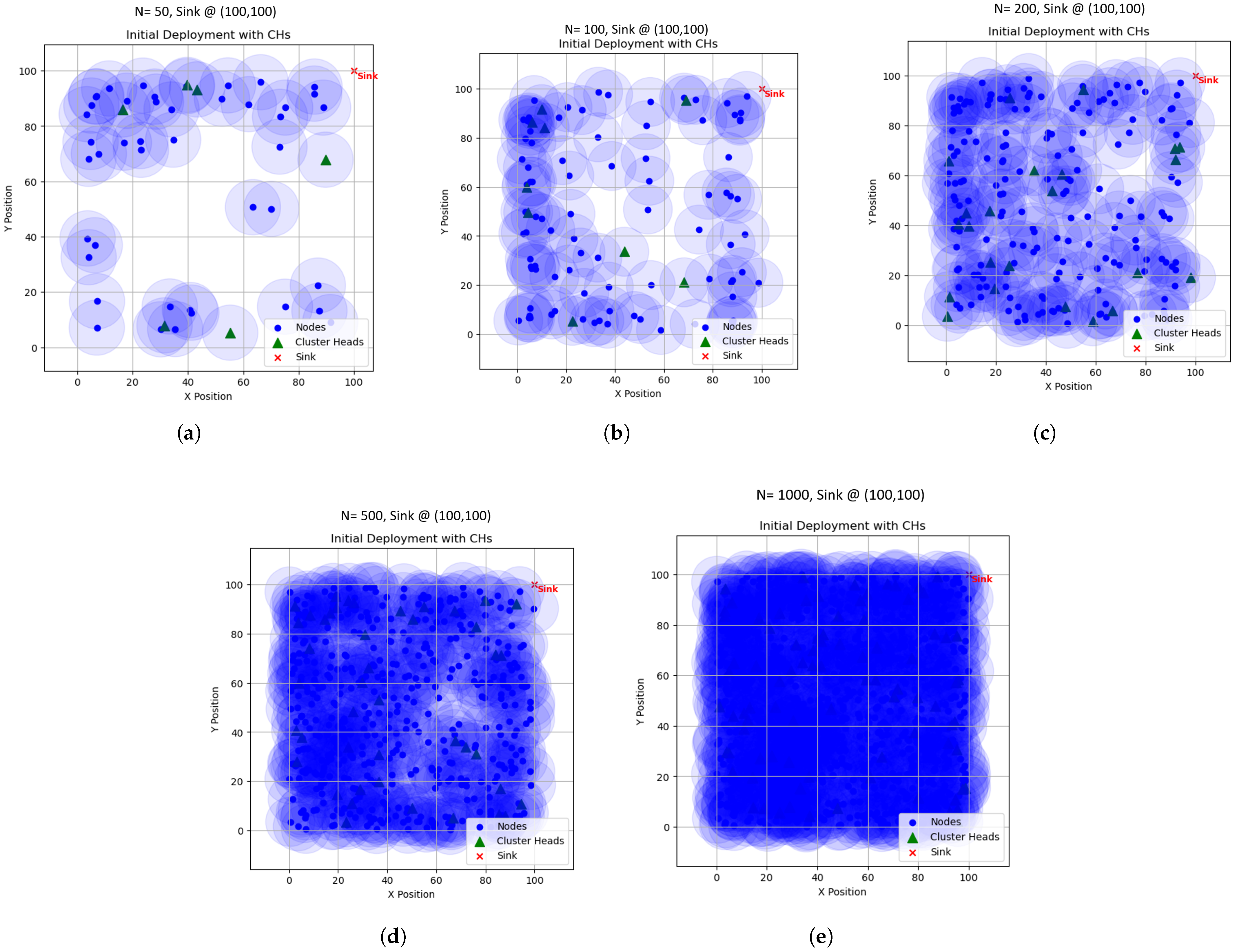
As shown in Figure 9, sensor nodes with different node densities were deployed in the field area of 100 × 100 m2, and the sink node or BS is placed at ( 100 , 100 ) to collect data from the CH. In particular, the disaster-based applications are more prone to node displacement or susceptible to dynamic changes, which require safe positioning of the sink node or BS. In the above mentioned deployment, a node density of 50, 100, 200, 500, and 1000 nodes is randomly deployed to monitor the area, but due to random deployment, most of the nodes leave some area unattended or uncovered, leading to coverage holes.
Specifically, 50- and 100-node deployments have a significant portion of the field left uncovered, which indicates inefficient coverage. In contrast, higher node densities like 200, 500, and 1000 cover most or all of the area, indicating near-complete coverage. The coverage is determined based on the nodes’ sensing range R s , the maximum area sensed by a sensor node, and its communication radius R c , a node’s maximum area to transmit data.
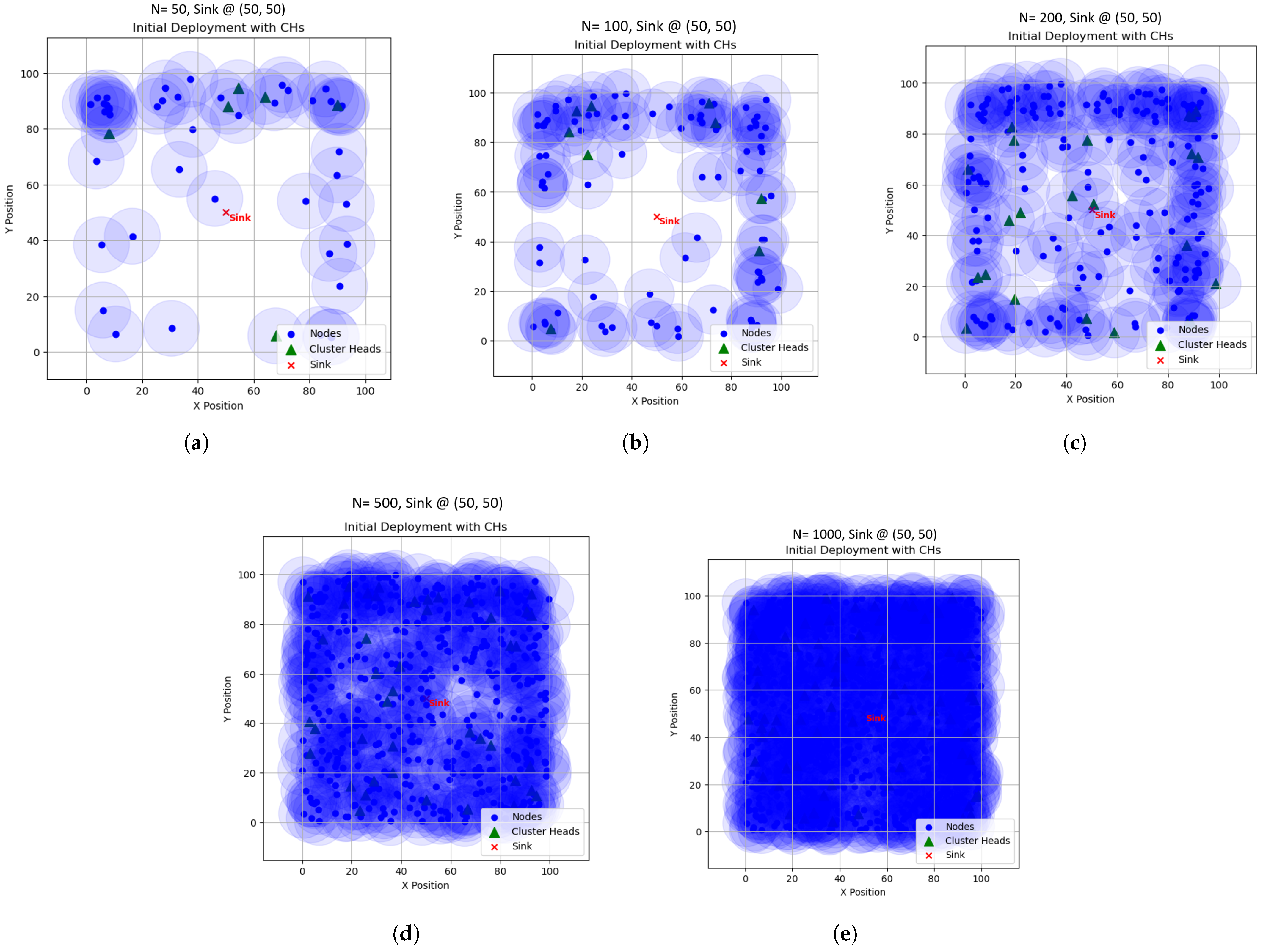
Similarly, Figure 10 shows the sensor nodes with different node densities deployed in the field area of 100 × 100 m2 with sink node or BS placed at ( 50 , 50 ) . Applications such as terrestrial monitoring, hospital monitoring, smart cities surveillance, and industrial area monitoring use this kind of BS deployment. As the sink location is in the center of the field area, which serves and gives equal reception importance to the field area, it efficiently connects and collects data from all directions fairly. As mentioned above, node densities of 50, 100, 200, 500, and 1000 were randomly deployed, with the sink node located at the center of the field area, which enables more efficient data reception compared to previous deployments and reduces energy consumption.
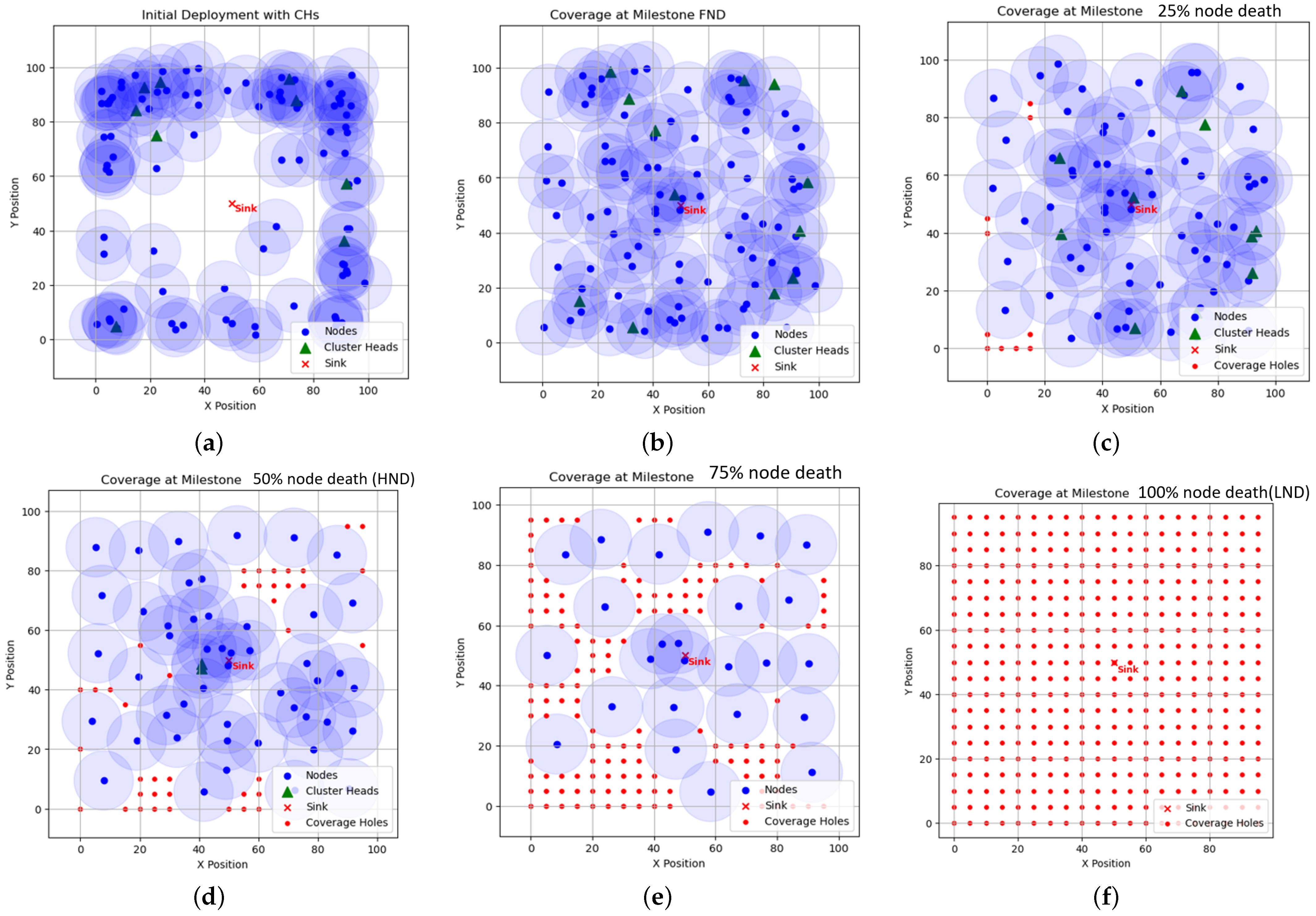
As shown in Figure 11, our proposed method HRHCOA with 100 nodes was deployed in the field area of 100 × 100 m2 with sink location at ( 50 , 50 ) . Figure 11a shows initial deployment of nodes with clusters formed by the LEACH protocol. The CHs in the clusters form a link between MNs and the sink node (BS) for data transmission. However, some areas remain unattended (coverage holes), leading to inefficiency. ROA utilizes its global exploration capability to identify optimal CHs and form new clusters, thereby reducing coverage holes. If some nodes still remain uncovered, selected MNs are relocated using HCO’s local refinement mechanism to cover these regions, and the data transmission process continues.
Further from Figure 11b–f shows the various milestones of future coverage holes formed at its FND, 25 % node death , HND 50 % node death , 75 % node death , and LND. At each round, coverage holes were calculated for network efficiency, and the coverage holes are cleared instantly, which improves coverage. This method is compared with LEACH, I-LEACH-EA, I-LEACH-DA-D, I-LEACH-DA-P, ROA, and HCO at different node densities of 50, 100, 200, 500, and 1000 nodes at both ( 100 , 100 ) and ( 50 , 50 ) sink locations.

6. Results

This section discusses the results obtained from the simulation for various densities at two different sink locations.
Table 6, Table 7, Table 8, Table 9, Table 10, Table 11, Table 12, Table 13, Table 14 and Table 15 show the comparison of various parameters such as node death at various levels, energy consumption E c , average delay, overall throughput, coverage ratio before and after healing for various node densities at two different sink locations.

6.1. Node Death Metrics

The node death metric identifies the round at which a node becomes inactive (dies). It also tells how fast and inconsistently their energy is consumed and marks a milestone to evaluate the network’s performance and its lifetime. From Table 6, Table 7, Table 8, Table 9, Table 10, Table 11, Table 12, Table 13, Table 14 and Table 15, our proposed HRHCOA method is compared with six different methods for their FND, HND, and LND with various node densities. For our proposed HRHCOA method, considering 1000 nodes with sink location at ( 100 , 100 ) , FND occurs at 317th round and goes till LND at (912th round. Similarly, for 50 nodes, I-LEACH-DA-Ps FND occurs at 71st round and LND at 490th round, whereas our proposed HRHCOAs FND happens at 288th round, which shows the stable start of the nodes transmission operation. Due to rapid hole formation at later rounds, LND for HRHCOA occurs at 564th round compared to HCOs 623rd and I-LEACH-DA-Ps 599th round. Further, for HRHCOA the FND occurs at 298th round and LND at 663rd round for 100 nodes, where HCOs LND occurs at 717th round and I-LEACH-DA-Ps LND at 722nd round. Due to continuous repositioning driven by HCO’s local refinement (exploitation) behavior, HRHCOA experiences slower performance compared to ROA and HCO. However, it still achieves moderately high performance, with 200 nodes showing FND at the 299th round and LND at the 805th round. For 500 nodes and 1000 nodes, LND is observed at the 874th round and 912th round, respectively.
Similarly, Table 6, Table 7, Table 8, Table 9, Table 10, Table 11, Table 12, Table 13, Table 14 and Table 15 represent the various node death levels of our proposed HRHCOA method with other methods deployed in a 100 × 100 field area with a sink node placed at ( 50 , 50 ) . Here, I-LEACH-DA-D performs low for all its densities in FND, HND, and LND levels as low as only 24 rounds for 1000 nodes and with a high LND of 1187 rounds for I-LEACH-DA-P in 1000 rounds. Here, our proposed HRHCOA methods perform slightly equal to LEACH, ROA, and HCO for FND at 760th round and accounts for 1139th round for HCO, 1096th round for ROA, and 1125th round for LEACH at 1000 nodes. Compared to sink location ( 100 , 100 ) , the sink location ( 50 , 50 ) deployment performs better. Most of the methods in this deployment perform similar, closer LNDs compared to the previous sink deployment.

6.2. Coverage Ratio

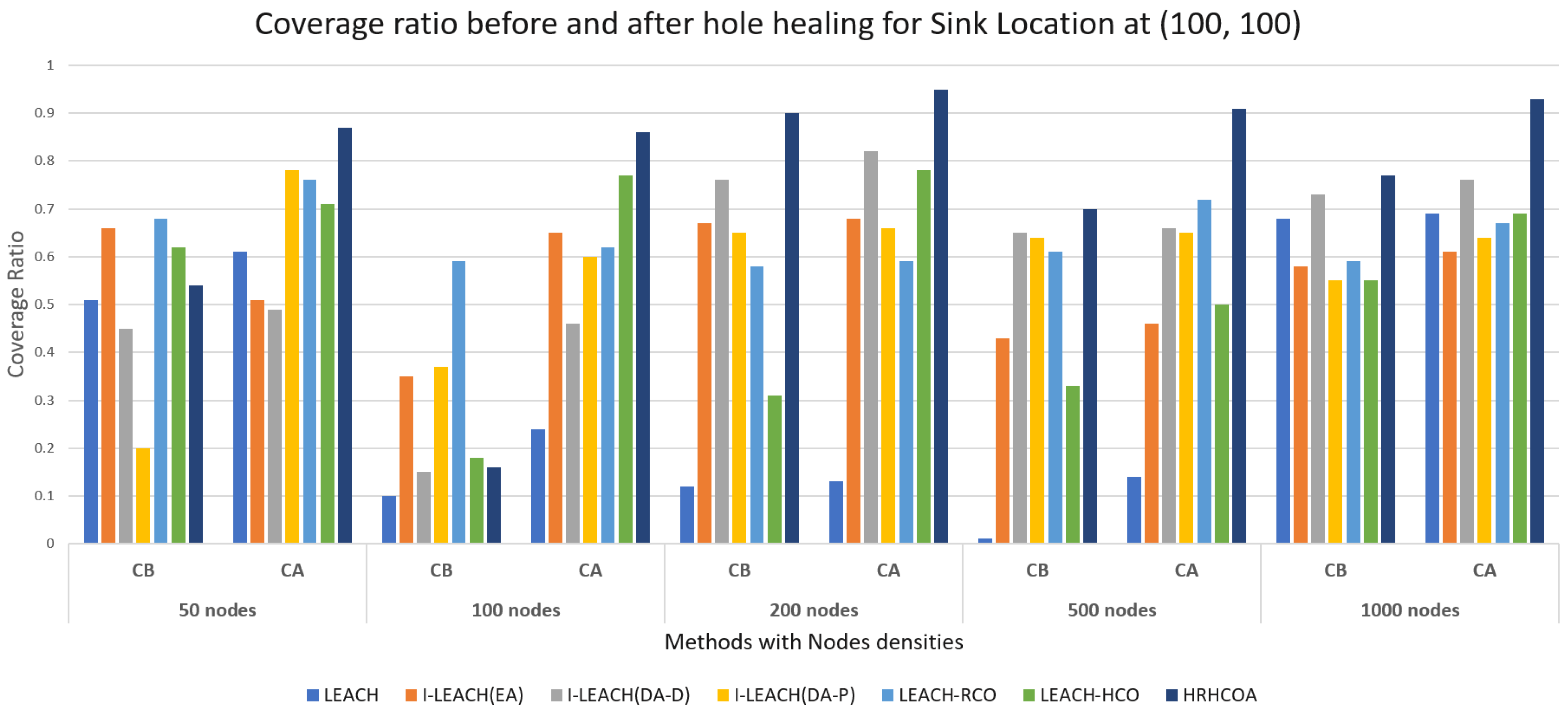
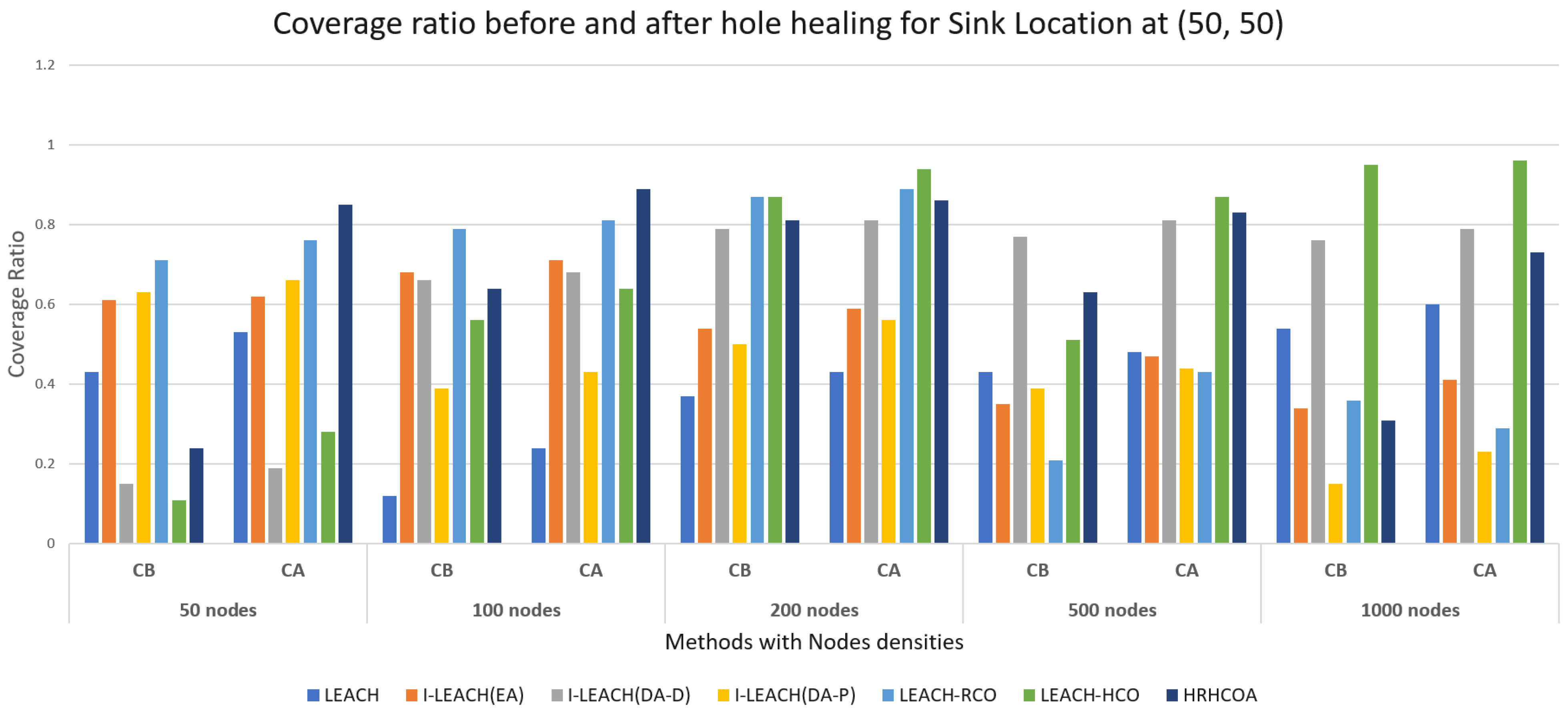
As shown in Figure 12 and Figure 13, the coverage ratios of nodes deployed with different node densities were plotted with the existing and proposed methods to heal the coverage holes formed. This metric combines coverage holes arising from initial deployment and those formed due to node failures, and evaluates the ratio of holes healed before and after each round by counting the number of unattended points in each grid sector. For the proposed method HRHCOA, considering 1000 nodes at sink location ( 100 , 100 ) , found the coverage hole ratio before mitigation as 77.05 % and 93.94 % after mitigation, accounting for an increase of 16.80 % , and for other densities 33.6 % , 69.79 % , 5.1 % and 20.63 % for 50, 100, 200, and 500 nodes, respectively. Similarly, for other existing methods, the coverage hole ratio before and after mitigation is calculated and compared with our proposed HRHCOA method to find the improvement in coverage. Similarly, at the sink location ( 50 , 50 ) and varying node densities, the coverage hole ratio before and after mitigation is evaluated. HRHCOA has an initial coverage ratio of 60.71 % , 25.39 % , 4.58 % , 20 % , and 41.78 % , but their initial coverage range and final coverage range from 24 % to 89 % , which are lower compared to the sink location scenario at ( 100 , 100 ) , where coverage ranges from 16 % to 95 % .

7. Performance Analysis

7.1. Throughput Metrics

Table 6, Table 7, Table 8, Table 9, Table 10, Table 11, Table 12, Table 13, Table 14 and Table 15 evaluate the overall throughput of different methods at various node densities and sink located at ( 100 , 100 ) and ( 50 , 50 ) . Even though in terms of node death, LEACH and its variants lived longer, they failed to deliver data bits efficiently. Our proposed HRHCOA method handled data transmission and transmitted maximum bits to the BS. Even for higher densities, HRHCOA performed well, and it was able to deliver around 3,139,192 bits for 1000 nodes, which is higher compared to other methods. In contrast, for the sink located at ( 50 , 50 ) and lower node densities (50 and 100), the proposed method delivers 174,536 bits and 349,514 bits, respectively, which are significantly higher than those of LEACH (28,000 bits and 75,021 bits) and I-LEACH-DA-D (25,218 bits and 61,043 bits). For higher densities like 500 and 1000 nodes, ROA, HCO, and HRHCOA have efficiently delivered bits to the BS, showing a higher efficiency. However, although I-LEACH-DA-P operates for a larger number of rounds, it delivers relatively low data to the BS, with 48,911 bits and 80,236 bits for 50 and 100 nodes, respectively. These values are significantly lower compared to ROA, HCO, and the proposed HRHCOA.

7.2. Delay Metrics

Table 6, Table 7, Table 8, Table 9, Table 10, Table 11, Table 12, Table 13, Table 14 and Table 15, compares the proposed methods delay metrics to the existing methods in delivering data to the BS, sink location at (100, 100). In this deployment, the sink is placed at a corner that increases the delay in transferring data from MNs to BS through CH. Our proposed method has to perform two processes in each round, such as selecting CH using ROA and the optimal node to reposition MNs using HCO to heal holes. Once this process is over, it transfers data, which includes a delay for the process and transferring data. Even though it takes time for this process, our proposed method performs fast with a low delay of 0.5209 s for 1000 nodes, 2.0405 s for 500, and 3.0721 s for 50 nodes at sink location ( 100 , 100 ) , which is low compared to LEACH variants and ROA. For lower densities, the proposed model performs better than all other existing methods.
Similarly, Table 6, Table 7, Table 8, Table 9, Table 10, Table 11, Table 12, Table 13, Table 14 and Table 15 show the delay metrics of each method compared with the proposed HRHCOA method with sink node deployed at ( 50 , 50 ) . As discussed earlier, the sink node is placed at the center of the field area, which ensures equal reception from all directions compared to far-end deployment. This reduces the time taken to deliver data from MNs to the sink via CHs. For lower density node deployments, the proposed HRHCOA has a slightly higher delay compared to HCO and ROA, and less than LEACH and its variants. Whereas, for higher densities, the delay is reduced, i.e., HRHCOA has 1.9039 s for 1000 nodes and 2.0405 s for 500 nodes, which is lower than LEACH and its variants, but the delay is higher compared to deployment at sink location ( 100 , 100 ) .

7.3. Energy Consumption in the Network

From Table 6, Table 7, Table 8, Table 9, Table 10, Table 11, Table 12, Table 13, Table 14 and Table 15, energy consumption E C of different node densities is compared with various methods at the sink node placed at ( 100 , 100 ) . In this deployment model, the sink node is placed at the far-end corner of the field area, which increases the energy consumption from the nodes that are deployed far away from the sink to send data from the MN to the sink via the CH nodes. The base methods like LEACH and its improved variants are mostly energy-aware and CH probabilistic, which are quite advantageous, but they easily fall into local traps and face high-energy consumption compared to bio-inspired models. For lower densities like 50 and 100 nodes, our proposed HRHCOA consumes a moderate level of energy E c as 0.1252 J, which is high compared to 0.1196 J of HCO and 0.1236 J of ROA and lower than LEACH and its variants. Whereas, for higher densities like 1000 nodes and 500 nodes, they consume 0.4453 J and 0.4854 J, respectively, for ROA and I-LEACH-DA-P, but I-LEACH-DA-D performs worst with 0.6944 J, the highest E c .
Similarly, Table 6, Table 7, Table 8, Table 9, Table 10, Table 11, Table 12, Table 13, Table 14 and Table 15 show the energy consumption E c for various node densities with sink location at (50, 50) using various methods like LEACH and its variants, ROA, HCO, and our proposed method HRHCOA. As the sink is placed in the center, the nodes, which are deployed at the farthest corner, need to spend little energy to transmit data to send to CH or CH to send data to the sink node. This makes the deployment more energy-efficient, but the hole formation in the network due to initial deployment and future holes due to node death contribute to energy consumption for rejoining the network. Here, compared to previous methods, HRHCOA exhibits lower energy consumption. For a 500-node deployment, the energy consumption is 0.2136 J, which is lower than that of LEACH, its variants, and ROA. Similarly, for 50 nodes, HRHCOA consumes 0.0307 J.

7.4. Limitations and Future Scope

Our proposed HRHCOA effectively maximizes coverage and reduces holes in WSNs efficiently by utilizing the global exploration (ROA) and local refining exploitation (HCO’s) behavior. Moreover, the HRHCOA method performs optimization metrics accurately to find holes and heal them. HRHCOA faces various challenges related to computational complexity, scalability, and energy efficiency. These are the major limitations that affect the performance in real-time deployments.
  • H i g h C o m p u t a t i o n a l C o s t : As it combines both (ROA and HCO) methods that increases iteration time and processing overheads.
  • E n e r g y O v e r h e a d s : At each round, whenever a hole emerges, immediately the HRHCOA algorithm tries to heal holes, which is unnecessary at that moment, and it consumes energy and reduces lifetime.
  • S c a l a b i l i t y : When the number of nodes is increased, it proportionally increases the search space, which causes slower convergence and lower accuracy even for identifying small holes.
  • H o l e D e t e c t i o n : At some instances, due to misalignment and miscalculation, it may leave out small or micro neighbor holes.
  • No mobile nodes or new additional nodes were added to reduce unattended area issues.
  • Optimization usually runs at a centralized database; if it fails suddenly, it will create a single point of failure in the network.
Considering the above limitations faced during the designing of the hybrid algorithm, these can be used to formulate future directions,
  • N e c e s s i t y b a s e d h o l e d e t e c t i o n : Ensure to heal hole only, if that is necessary in that particular round. If not, proceed till necessity arrives.
  • E n e r g y b a s e d M o d e l i n g : Healing in each round increases burden, and choosing a node based on residual energy alone is not sufficient, but we need to look at other parameters associated with it.
  • M u l t i o b j e c t i v e o p t i m i z a t i o n : Fitness evaluation functions like coverage, delay, residual energy levels, and stable connectivity need to be considered more sensitive during designing optimization techniques.
  • Choosing optimized energy threshold to select optimal CH for efficient clustering.

8. Conclusions

The proposed HRHCOA method introduces an efficient and intelligent approach to achieve maximum coverage and balanced energy operation in Wireless Sensor Networks (WSNs). By integrating the global exploration capability of ROA with the local exploitation behavior of HCO, the method improves optimal cluster head (CH) selection, ensures stable CH operation for a longer duration, balances energy consumption, and supports adaptive coverage hole recovery. The HRHCOA method not only detects and heals coverage holes formed during the initial deployment but also dynamically adapts to improve the coverage ratio when future holes occur due to node failures or energy depletion. The algorithm is evaluated under different simulation scenarios for varying node densities of 50, 100, 200, 500, and 1000 and its sink is located at ( 100 , 100 ) and ( 50 , 50 ) . Performance of the proposed method is analyzed using metrics such as first node death, half node death, last node death, average energy consumption, average delay, overall throughput, and coverage ratio before and after node relocation. For the sink location at (100,100), there is an increase in network lifetime of 65% for 1000 nodes, and these results demonstrate that the proposed algorithm has an increased throughput of 3,139,293 bits, reduced delay of 2.2792 s and maximized coverage ratio of 16.93% from 77.05% to 93.94% compared to the Hermit-Crab Optimization Algorithm, Raccoon Optimization Algorithm, LEACH, and its variants, including I-LEACH energy-aware, I-LEACH distance-aware deterministic, and I-LEACH distance-aware probabilistic techniques. Consequently, HRHCOA enhances network stability and extends overall network lifetime.
In the future, it is necessary to design a more effective energy-based coverage hole detection and mitigation algorithm, only when the coverage ratio falls below a certain threshold, instead of healing in every simulation round. By employing adaptive multi-objective optimization models to overcome constraints in fitness functions, the performance of the optimization algorithms can be improved further.

Author Contributions

Conceptualization, S.L.R.B.; methodology, S.L.R.B.; software, S.L.R.B.; validation, S.L.R.B. and R.D.S.; formal analysis, S.L.R.B.; investigation, S.L.R.B. and R.D.S.; resources, S.L.R.B.; data curation, S.L.R.B. and R.D.S.; writing—original draft preparation, S.L.R.B.; writing—review and editing, S.L.R.B. and R.D.S.; visualization, S.L.R.B.; supervision, R.D.S.; All authors have read and agreed to the published version of the manuscript.

Funding

This research received no external funding.

Data Availability Statement

Data is contained within the article.

Conflicts of Interest

The authors declare no conflicts of interest.

Abbreviations

Mathematical Symbols and Notations used.
Symbol/ NotationDescription
E t x Transmission energy
E r x Received energy
E o Initial energy
E e l e c Energy spent by electronics
ϵ a m p Amplification energy
E m o v e Energy spent to move
E D A Energy spent for data aggregation
P i initial population
P h Population based on hole
C n e w Coverage new (updated coverage)
C o l d Coverage old (previous coverage)
HHole in the network
w n tunable weights for fitness
X n Best value
C H t h Cluster head Threshold
C H k Cluster head updated value based on CH number
b e s t i population best solution value
α Directed movement of the node of the Hermit crab
δ Adaptive random shifting of Hermit crab movement
γ Global best value of Raccoons for optimal Ch
η Local refining best value of Den selection by a raccoon
R S Sensing range of the node
R C Communication range of a node

References

  1. Kandris, D.; Nakas, C.; Vomvas, D.; Koulouras, G. Applications of Wireless Sensor Networks: An Up-to-Date Survey. Appl. Syst. Innov. 2020, 3, 14. [Google Scholar] [CrossRef]
  2. Carlos-Mancilla, M.; López-Mellado, E.; Siller, M. Wireless Sensor Networks Formation: Approaches and Techniques. J. Sens. 2016, 2016, 2081902. [Google Scholar] [CrossRef]
  3. Angelin, A.C.; Silas, S. A Comparative Study of Coverage Hole Detection Techniques in Wireless Sensor Networks. Eng. Proc. 2023, 59, 5. [Google Scholar]
  4. Heinzelman, W.R.; Chandrakasan, A.; Balakrishnan, H. Energy-Efficient Communication Protocol for Wireless Microsensor Networks. In 33rd Annual Hawaii International Conference on System Sciences; IEEE: Piscataway, NJ, USA, 2000; p. 10. [Google Scholar]
  5. Sushil, L.; Satvir, S. Enhancing Energy Efficiency in Wireless Sensor Networks through I-LEACH: A Data Clustering and Routing Protocol. J. Electr. Syst. 2024, 20, 81–91. [Google Scholar]
  6. Gautam, N.; Pyun, J.Y. Distance Aware Intelligent Clustering Protocol for Wireless Sensor Networks. J. Commun. Netw. 2010, 12, 122–129. [Google Scholar] [CrossRef]
  7. Devi, S.; Sangwan, A. Genetic Algorithm-Based Coverage Maximization and Connectivity Preserving Approach Using Computational Geometry for 3-Dimensional Directional Sensor Networks. Int. J. Electron. Commun. Eng. 2025, 12, 22–39. [Google Scholar] [CrossRef]
  8. Bhargavi, K.V.N.A.; Varma, G.P.S.; Hemalatha, I.; Dilli, R. An Enhanced Particle Swarm Optimization-Based Node Deployment and Coverage in Sensor Networks. Sensors 2024, 24, 6238. [Google Scholar] [CrossRef] [PubMed]
  9. Yan, L.; He, Y.; Huangfu, Z. A Fish Swarm Inspired Holes Recovery Algorithm for Wireless Sensor Networks. Int. J. Wirel. Inf. Netw. 2020, 27, 89–101. [Google Scholar] [CrossRef]
  10. Onuzulike, V.C.; Nwabueze, C.A.; Obidike, A.I.; Ebih, U. Coverage Hole Detection in Embedded Wireless Sensor Network Using ACO Based Technique: Comparative Architecture. Int. J. Res. Eng. Sci. (IJRES) 2023, 11, 239–246. [Google Scholar]
  11. Wen, Q.; Zhao, X.Q.; Cui, Y.P.; Zeng, Y.P.; Chang, H.; Fu, Y.J. Coverage Enhancement Algorithm for WSNs Based on Vampire Bat and Improved Virtual Force. IEEE Sens. J. 2022, 22, 8245–8256. [Google Scholar] [CrossRef]
  12. Dey, R.; Thakurta, P.K.G.; Kar, S. Efficient Energy Aware Area Coverage in WSNs: A 2L-Voronoi Guided PSO Approach. In OPSEARCH; Springer: Berlin/Heidelberg, Germany, 2024; pp. 1–31. [Google Scholar]
  13. Khamlichi, Y.E.; Mesmoudi, Y.; Tahiri, A.; Abtoy, A. A Recovery Algorithm to Detect and Repair Coverage Holes in Wireless Sensor Network System. J. Commun. 2018, 13, 67–74. [Google Scholar] [CrossRef]
  14. Li, W.; Zhang, W. Coverage Hole and Boundary Nodes Detection in Wireless Sensor Networks. J. Netw. Comput. Appl. 2015, 48, 35–43. [Google Scholar] [CrossRef]
  15. Kumar Sahoo, P.; Chiang, M.J.; Wu, S.L. An Efficient Distributed Coverage Hole Detection Protocol for Wireless Sensor Networks. Sensors 2016, 16, 386. [Google Scholar] [CrossRef]
  16. Nguyen, D.T.; Nguyen, N.P.; Thai, M.T.; Helal, A. An Optimal Algorithm for Coverage Hole Healing in Hybrid Sensor Networks. 7th International Wireless Communications and Mobile Computing Conference; IEEE: Piscataway, NJ, USA, 2011; pp. 494–499. [Google Scholar][Green Version]
  17. Zhuang, Y.; Wu, C.; Wu, H.; Chu, H.; Gao, Y.; Li, L. The Repair Strategy for Event Coverage Holes Based on Mobile Robots in Wireless Sensor and Robot Networks. Sensors 2019, 19, 5045. [Google Scholar] [CrossRef] [PubMed]
  18. Al-Sodairi, S.; Ouni, R. Reliable and Energy-Efficient Multi-Hop LEACH-Based Clustering Protocol for Wireless Sensor Networks. Sustain. Comput. Inform. Syst. 2018, 20, 1–13. [Google Scholar] [CrossRef]
  19. Narayan, V.; Daniel, A.K. CHOP: Maximum Coverage Optimization and Resolve Hole Healing Problem Using Sleep and Wake-Up Technique for WSN. ADCAIJ Adv. Distrib. Comput. Artif. Intell. J. 2022, 11, 159. [Google Scholar] [CrossRef]
  20. Krishna, K.R.; Mohan, K.R. Hole Detection and Hole Healing in a Wireless Sensor Network Using LeDiR Methodology. Indian J. Sci. Technol. 2016, 9, 1–9. [Google Scholar] [CrossRef]
  21. Thakkar, A. DEAL: Distance and Energy Based Advanced LEACH Protocol. In Proceedings of the International Conference on Information and Communication Technology for Intelligent Systems; Springer International Publishing: Berlin/Heidelberg, Germany, 2017; pp. 370–376. [Google Scholar]
  22. Wang, F.; Hu, H. Symmetric Algorithm for Detection of Coverage Hole in Wireless Sensor Network. Wirel. Pers. Commun. 2022, 127, 141–158. [Google Scholar] [CrossRef]
  23. Suleiman, H.; Hamdan, M. Adaptive Probabilistic Model for Energy-Efficient Distance-Based Clustering in WSNs (Adapt-P): A LEACH-Based Analytical Study. arXiv 2021, arXiv:2110.13300. [Google Scholar]
  24. Yoon, C.; Cho, S.; Lee, Y. Extending WSN Lifetime with Enhanced LEACH Protocol in Autonomous Vehicle Using Improved K-Means and Advanced Cluster Configuration Algorithms. Appl. Sci. 2024, 14, 11720. [Google Scholar] [CrossRef]
  25. Wang, J.; Ju, C.; Gao, Y.; Kim, G.J. A PSO Based Energy Efficient Coverage Control Algorithm for Wireless Sensor Networks. Comput. Mater. Contin. 2018, 56, 433–446. [Google Scholar]
  26. Siamantas, G.; Kandris, D. Particle Swarm Optimization for K-Coverage and 1-Connectivity in Wireless Sensor Networks. Electronics 2024, 13, 4841. [Google Scholar] [CrossRef]
  27. Sekyere, Y.O.; Effah, F.B.; Okyere, P.Y. An Enhanced Particle Swarm Optimization Algorithm via Adaptive Dynamic Inertia Weight and Acceleration Coefficients. J. Electron. Electr. Eng. 2024, 3, 53–67. [Google Scholar]
  28. Zhao, Q.; Li, C.; Zhu, D.; Xie, C. Coverage Optimization of Wireless Sensor Networks Using Combinations of PSO and Chaos Optimization. Electronics 2022, 11, 853. [Google Scholar] [CrossRef]
  29. Elhoseny, M.; Tharwat, A.; Yuan, X.; Hassanien, A.E. Optimizing K-Coverage of Mobile WSNs. Expert Syst. Appl. 2018, 92, 142–153. [Google Scholar] [CrossRef]
  30. Larhlimi, I.; Lmkaiti, M.; Lachgar, M.; Ouchitachen, H.; Darif, A.; Mouncif, H. Genetic Algorithm-Driven Cover Set Scheduling for Longevity in Wireless Sensor Networks. Int. J. Adv. Comput. Sci. Appl. 2025, 16, 1104–1112. [Google Scholar] [CrossRef]
  31. Hanh, N.T.; Binh, H.T.T.; Hoai, N.X.; Palaniswami, M.S. An Efficient Genetic Algorithm for Maximizing Area Coverage in Wireless Sensor Networks. Inf. Sci. 2019, 488, 58–75. [Google Scholar] [CrossRef]
  32. Vishal, P. Deployment of Context-Aware Sensor in Wireless Sensor Network Based on the Variants of Genetic Algorithm. Int. J. Artif. Life Res. (IJALR) 2018, 8, 1–24. [Google Scholar] [CrossRef]
  33. Zain Eldin, H.; Badawy, M.; Elhosseini, M.; Arafat, H.; Abraham, A. An Improved Dynamic Deployment Technique Based on Genetic Algorithm (IDDT-GA) for Maximizing Coverage in Wireless Sensor Networks. J. Ambient Intell. Humaniz. Comput. 2020, 11, 4177–4194. [Google Scholar] [CrossRef]
  34. Tian, J.; Gao, M.; Ge, G. Wireless Sensor Network Node Optimal Coverage Based on Improved Genetic Algorithm and Binary Ant Colony Algorithm. EURASIP J. Wirel. Commun. Netw. 2016, 2016, 104. [Google Scholar] [CrossRef]
  35. Kurian, A.M.; Onuorah, M.J.; Ammari, H.M. Optimizing Coverage in Wireless Sensor Networks: A Binary Ant Colony Algorithm with Hill Climbing. Appl. Sci. 2024, 14, 960. [Google Scholar] [CrossRef]
  36. Jaiswal, K.; Anand, V. A QoS Aware Optimal Node Deployment in Wireless Sensor Network Using Grey Wolf Optimization Approach for IoT Applications. Telecommun. Syst. 2021, 78, 559–576. [Google Scholar] [CrossRef]
  37. Ou, Y.; Qin, F.; Zhou, K.Q.; Yin, P.F.; Mo, L.P.; Mohd Zain, A. An Improved Grey Wolf Optimizer with Multi-Strategies Coverage in Wireless Sensor Networks. Symmetry 2024, 16, 286. [Google Scholar] [CrossRef]
  38. Bashyam, S.L.R.; Subramanian, R.D.; Chandra, J. An Efficient Node-to-Node Coverage and Connectivity with RSSI Using Grey-Wolf Prediction Optimization Algorithm in Remote Low Accessibility Area. In 2023 2nd International Conference on Vision Towards Emerging Trends in Communication and Networking Technologies (ViTECoN); IEEE: Piscataway, NJ, USA, 2023; pp. 1–6. [Google Scholar]
  39. Xu, Y.; Zhang, B.; Zhang, Y. Application of an Enhanced Whale Optimization Algorithm on Coverage Optimization of Sensor. Biomimetics 2023, 8, 354. [Google Scholar] [CrossRef] [PubMed]
  40. Huang, Y.; Zhang, J.; Wei, W.; Qin, T.; Fan, Y.; Luo, X.; Yang, J. Research on Coverage Optimization in a WSN Based on an Improved COOT Bird Algorithm. Sensors 2022, 22, 3383. [Google Scholar] [CrossRef]
  41. Zeng, C.; Qin, T.; Tan, W.; Lin, C.; Zhu, Z.; Yang, J.; Yuan, S. Coverage Optimization of Heterogeneous Wireless Sensor Network Based on Improved Wild Horse Optimizer. Biomimetics 2023, 8, 70. [Google Scholar] [CrossRef] [PubMed]
  42. Kadoke, K.M.; Goyal, S.; Kaur, R. The Jellyfish Algorithm: A New Approach for Enhancing Coverage, Reducing Energy Consumption, and Extending Network Lifetime in Underwater Wireless Sensor Networks. J. Electr. Syst. Inf. Technol. 2025, 12, 68. [Google Scholar] [CrossRef]
  43. Kim, J.; Yoo, Y. Sensor Node Activation Using Bat Algorithm for Connected Target Coverage in WSNs. Sensors 2020, 20, 3733. [Google Scholar] [CrossRef]
  44. Subburathinam, K.; Bakthavatchalam, V.; Pandian, R.K.C.; Subramaniam, K.M. Enhancing Wireless Sensor Network Connectivity and Coverage Using Hybrid GWO-HSA Algorithm. Int. J. Commun. Syst. 2024, 37, e5858. [Google Scholar] [CrossRef]
  45. Bourebia, N.E.H.; Li, C. A Novel Raccoon Optimization Algorithm with Multi-Objective Clustering Strategy Based Routing Protocol for WSNs. Peer-to-Peer Netw. Appl. 2023, 16, 1624–1640. [Google Scholar] [CrossRef]
  46. Bashyam, S.L.R.; Subramanian, R.D. Hermit Crab Optimization to Overcome Coverage Hole Issue for Efficient Hole Issue in WSN. In 2024 International Conference on Electrical Electronics and Computing Technologies (ICEECT); IEEE: Piscataway, NJ, USA, 2024; Volume 1, pp. 1–8. [Google Scholar]
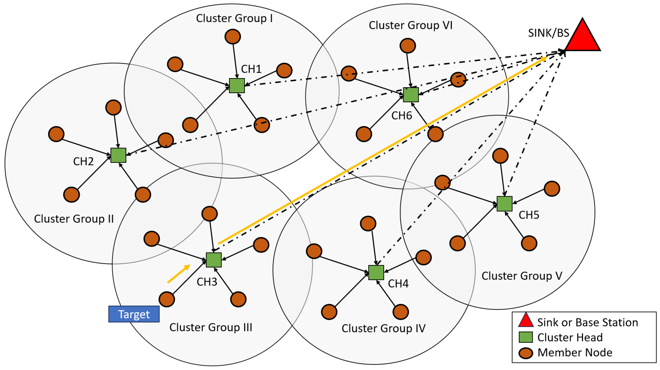
Figure 1. A typical wireless sensor network (WSN) architecture.
Futureinternet 18 00163 g001
Figure 2. Sensor node deployment: (a) LEACH-based clustering. (b) A new cluster formed after a few nodes death.
Futureinternet 18 00163 g002
Figure 3. First- order radio model (Energy).
Futureinternet 18 00163 g003
Figure 4. Node A’s repositioning from one position to another.
Futureinternet 18 00163 g004
Figure 5. Foraging and den relocation behavior of raccoons.
Futureinternet 18 00163 g005
Figure 6. Hermit crabs shell finding and repositioning behavior.
Futureinternet 18 00163 g006
Figure 7. A typical representation of the proposed Hybrid Raccoon–Hermit Crab Optimization Algorithm (HRHCOA).
Futureinternet 18 00163 g007
Figure 8. Flowchart of Hybrid Raccoon–Hermit Crab Optimization Algorithm.
Futureinternet 18 00163 g008
Figure 9. Initial node deployment in the field area of 100 × 100 m2 and sink location at ( 100 , 100 ) . (a) For 50 nodes. (b) For 100 nodes. (c) For 200 nodes. (d) For 500 nodes. (e) For 1000 nodes.
Futureinternet 18 00163 g009
Figure 10. Initial node deployment in the field area of 100 × 100 m2 and sink location at ( 50 , 50 ) . (a) For 50 nodes. (b) For 100 nodes. (c) For 200 nodes. (d) For 500 nodes. (e) For 1000 nodes.
Futureinternet 18 00163 g010
Figure 11. Results of proposed HRHCOA: Deployment milestone at various node death stages of 100 × 100 m2 and sink location at ( 50 , 50 ) . (a) Initial deployment. (b) Deployment at FND. (c) Deployment at 25 % node death. (d) Deployment at HND. (e) Deployment at 75 % node death. (f) Final stage total node death.
Futureinternet 18 00163 g011
Figure 12. Comparison of coverage ratio of various node densities 50, 100, 200,500 and 1000 nodes with various methods and proposed method with sink location at (100, 100).
Futureinternet 18 00163 g012
Figure 13. Comparison of coverage ratio of various node densities 50, 100, 200,500 and 1000 nodes with various methods and proposed method with sink location at (50, 50).
Futureinternet 18 00163 g013
Table 4. Tabulation of coverage holes before and after mitigation at each round (area = 100 × 100, n = 1000, sink = (100, 100), Rs = 10, Rc = 15, rounds = 1500, Eo = 0.5 J, Etx = Erx = 50 nJ, Eda = 100 nJ).
Rounds/MetricsNodes DepletedCoverage Hole Before MitigationCoverage Hole After Mitigation
0Initial31
1100000
50100000
100100000
150100000
200100000
250100000
300100000
312399 (FND)00
35099900
40099500
45098100
50094910
55087630
60079211
6506831412
7005691713
730500 (HND)2018
7504503937
8003233635
850191119111
90011309308
9102375373
9111386381
9120 (LND)400400
9130400400
Table 5. Parametic table for WSN deployment.
Metric/ScenarioIIIIIIIVV
Field Size 100 × 100 100 × 100 100 × 100 100 × 100 100 × 100
No. of Nodes501002005001000
Radio ModelEnergy–Mobilty modelEnergy–Mobilty modelEnergy–Mobilty modelEnergy–Mobilty modelEnergy–Mobilty model
Sink location(100, 100) (50, 50)(100, 100) (50, 50)(100, 100) (50, 50)(100, 100) (50, 50)(100, 100) (50, 50)
Sensing range R s 1010101010
Comm range R c 1515151515
E o (J)2 J2 J2 J2 J2 J
E e l e c (J)50 nJ50 nJ50 nJ50 nJ50 nJ
E t x 0.0073 nJ0.0073 nJ0.0073 nJ0.0073 nJ0.0073 nJ
E r x 0.0054 nJ0.0054 nJ0.0054 nJ0.0054nJ0.0054 nJ
E D A 100 pJ100 pJ100 pJ100 pJ100 pJ
C H P r o b a b i l i t y 10%10%10%10%10%
Packet size (k)40004000400040004000
Rounds15001500150015001500
Table 6. Comparison of performance metrics of various methods with proposed hybrid model for (Area = 100 × 100, n = 50, sink = (100, 100), Rs = 10, Rc = 15, rounds = 1500, Eo = 0.5 J, Etx = Erx = 50 nJ, Eda = 100 nJ).
Metrics/MethodLEACHI-LEACH (EA)I-LEACH (DA-D)I-LEACH (DA-P)ROAHCOAHRHCOA
FND27816971314278235288
HND478375248512479539456
LND566453490599566623564
Average Ec0.04430.05510.05100.04170.04430.04010.0445
Average Delay4.67735.38455.85754.38674.68674.09584.4878
Overall Throughput23,11317,72413,95024,92262,98974,632158,709
CR Before (in %)51.2566.2045.2020.5168.9062.1054.21
CR After (in %)61.4067.1049.9078.2476.9871.3887.81
Table 7. Comparison of performance metrics of various methods with proposed hybrid model for (Area = 100 × 100, n = 100, sink = (100, 100), Rs = 10, Rc = 15, rounds = 1500, Eo = 0.5 J, Etx = Erx = 50 nJ, Eda = 100 nJ).
Metrics/MethodLEACHI-LEACH (EA)I-LEACH (DA-D)I-LEACH (DA-P)ROAHCOAHRHCOA
FND32717063411328371298
HND591532323628592623564
LND697580543722675717663
Average Ec0.07210.08620.00920.06910.07100.06570.0559
Average Delay3.7204.42405.60673.60233.91043.46503.0028
Overall Throughput57,25847,72531,77032,80262,35379,73583,406
CR Before (in %)10.7435.7115.4437.6959.8218.9516.45
CR After (in %)24.8365.1246.5162.9860.2777.0786.24
Table 8. Comparison of performance metrics of various methods with proposed hybrid model for (Area = 100 × 100, n = 200, sink = (100, 100), Rs = 10, Rc = 15, rounds = 1500, Eo = 0.5 J, Etx = Erx = 50 nJ, Eda = 100 nJ).
Metrics/MethodLEACHI-LEACH (EA)I-LEACH (DA-D)I-LEACH (DA-P)ROAHCOAHRHCOA
FND38819237522376336299
HND645622359738676685672
LND802674477849816836805
Average Ec0.17620.14830.16660.14770.12360.11960.1252
Average Delay4.00123.90625.31213.97003.43302.89493.0721
Overall Throughput131,109112,247170,628147,659641,710632,861647,498
CR Before (in %)12.4367.4376.6365.1758.7531.2690.30
CR After (in %)13.7568.7582.3166.0559.7178.4895.40
Table 9. Comparison of performance metrics of various methods with proposed hybrid model for (Area = 100 × 100, n = 500, sink = (100, 100), Rs = 10, Rc = 15, rounds = 1500, Eo = 0.5 J, Etx = Erx = 50 nJ, Eda = 100 nJ).
Metrics/MethodLEACHI-LEACH (EA)I-LEACH (DA-D)I-LEACH (DA-P)ROAHCOAHRHCOA
FND39320825627375384374
HND705655358803705708705
LND868734660948879908874
Average Ec0.35210.34050.37870.36370.31740.27530.2892
Average Delay2.97423.67505.05452.89742.67762.41682.5732
Overall Throughput346,320300,462184,857406,0081,573,6971,530,0171,581,633
CR Before (in %)01.2443.1565.7064.6261.1333.1570.79
CR After (in %)14.2146.1566.2165.4772.3250.3991.53
Table 10. Comparison of performance metrics of various methods with proposed hybrid model for (Area = 100 × 100, n = 1000, sink = (100, 100), Rs = 10, Rc = 15, rounds = 1500, Eo = 0.5 J, Etx = Erx = 50 nJ, Eda = 100 nJ).
Metrics/MethodLEACHI-LEACH (EA)I-LEACH (DA-D)I-LEACH (DA-P)ROAHCOAHRHCOA
FND34724510647318317317
HND701691369862729731730
LND9088077201030928932912
Average Ec0.50600.61950.69440.68540.64530.53640.5029
Average Delay3.12103.49104.85842.92002.32542.29602.2792
Overall Throughput718,861650,828387,672867,3071,688,1053,089,2093,139,293
CR Before (in %)68.7158.6373.1255.6159.2155.6177.05
CR After (in %)69.3161.2776.2364.2367.8269.5393.94
Table 11. Comparison of performance metrics of various methods with proposed hybrid model for (Area = 100 × 100, n = 50, sink = (50, 50), Rs = 10, Rc = 15, rounds = 1500, Eo = 0.5 J, Etx = Erx = 50 nJ, Eda = 100 nJ).
Metrics/MethodLEACHI-LEACH (EA)I-LEACH (DA-D)I-LEACH (DA-P)ROAHCOAHRHCOA
FND347314124465348277389
HND574536571678576613566
LND747567731704749762630
Average Ec0.03350.04400.34190.03550.03460.03280.0307
Average Delay3.85114.46604.26513.78693.73473.56043.9021
Overall Throughput28,00025,21826,86048,911149,665159,569174,356
CR Before (in %)43.2961.6515.4263.5771.4301.1424.71
CR After (in %)53.7462.9319.7466.4176.5728.5585.42
Table 12. Comparison of performance metrics of various methods with proposed hybrid model for (Area = 100 × 100, n = 100, sink = (50, 50), Rs = 10, Rc = 15, rounds = 1500, Eo = 0.5 J, Etx = Erx = 50 nJ, Eda = 100 nJ).
Metrics/MethodLEACHI-LEACH (EA)I-LEACH (DA-D)I-LEACH (DA-P)ROAHCOAHRHCOA
FND49933290576500521472
HND764669652765819777753
LND850691819843850894845
Average Ec0.05900.07230.06100.05930.05800.05590.0519
Average Delay3.32893.75293.90363.12033.02892.99223.0618
Overall Throughput75,02161,04360,45980,236352,569340,890349,514
CR Before (in %)12.5668.8966.4939.7179.4256.8464.32
CR After (in %)24.8971.0468.4243.5181.0268.9189.71
Table 13. Comparison of performance metrics of various methods with proposed hybrid model for (Area = 100 × 100, n = 200, sink = (50, 50), Rs = 10, Rc = 15, rounds = 1500, Eo = 0.5 J, Etx = Erx = 50 nJ, Eda = 100 nJ).
Metrics/MethodLEACHI-LEACH (EA)I-LEACH (DA-D)I-LEACH (DA-P)ROAHCOAHRHCOA
FND59633660653597605606
HND924742761992925924916
LND10057619591133100510181008
Average Ec0.10000.13140.10420.10080.10000.09230.1008
Average Delay2.59173.37203.45792.55502.49172.47982.4583
Overall Throughput180,531134,620137,587191,550717,735724,892720,004
CR Before (in %)37.4254.8779.9250.4887.4587.7581.73
CR After (in %)43.2359.1181.6856.7289.1894.9386.31
Table 14. Comparison of performance metrics of various methods with proposed hybrid model for (Area = 100 × 100, n = 500, sink = (50, 50), Rs = 10, Rc = 15, rounds = 1500, Eo = 0.5 J, Etx = Erx = 50 nJ, Eda = 100 nJ).
Metrics/MethodLEACHI-LEACH (EA)I-LEACH (DA-D)I-LEACH (DA-P)ROAHCOAHRHCOA
FND70644646930707734706
HND1004821819106010057091010
LND10898481085111710649081089
Average Ec0.23140.29480.23040.22380.21450.20530.2136
Average Delay2.16242.98603.01692.14732.16252.01682.0405
Overall Throughput492,964385,831373,961529,0021,808,8661,930,0172,107,592
CR Before (in %)43.9135.0877.8239.0321.4151.3063.39
CR After (in %)48.9147.3181.3944.7843.1887.5783.28
Table 15. Comparison of performance metrics of various methods with proposed hybrid model for (Area = 100 × 100, n = 1000, sink = (50, 50), Rs = 10, Rc = 15, rounds = 1500, Eo = 0.5 J, Etx = Erx = 50 nJ, Eda = 100 nJ).
Metrics/MethodLEACHI-LEACH (EA)I-LEACH (DA-D)I-LEACH (DA-P)ROAHCOAHRHCOA
FND76064724935760760760
HND10319508301106103210291031
LND112599711301187109611391129
Average Ec0.44910.50150.44240.42120.39410.38980.3477
Average Delay1.92752.50752.82741.92881.92751.89481.9039
Overall Throughput1,014,673922,848759,9381,102,1513,604,1703,860,2283,589,427
CR Before (in %)54.3234.7176.1715.4936.0495.3231.34
CR After (in %)60.4141.7879.7423.6429.8196.5173.12
Disclaimer/Publisher’s Note: The statements, opinions and data contained in all publications are solely those of the individual author(s) and contributor(s) and not of MDPI and/or the editor(s). MDPI and/or the editor(s) disclaim responsibility for any injury to people or property resulting from any ideas, methods, instructions or products referred to in the content.