LeapNP: A Modular Python Framework for Benchmarking Learned Heuristics in Numeric Planning ^†

Abstract

This paper introduces LeapNP (Learning and Planning Framework for Numeric Problems), a lightweight, Python-native framework engineered to support both classical and numeric planning tasks. Designed with a fully modular interface, it specifically aims to facilitate the seamless integration of deep learning methodologies. The design philosophy of LeapNP stems from the observation that traditional planners, while highly efficient, lack the necessary flexibility for experimental research, particularly at the intersection of learning and planning. Most state-of-the-art engines are built as highly optimized, rigid executables that are resistant to internal modification. LeapNP disrupts this paradigm by offering a framework where the entire planning stack is accessible and mutable. Users can seamlessly plug in custom implementations for grounding, define novel state representations, or design bespoke search strategies, thereby enabling a level of integration with learning models that is currently impractical with standard tools. By significantly lowering the engineering barrier, our planner fosters rapid experimentation and accelerates research in neuro-symbolic planning. We also present a comprehensive suite of search algorithms, designed to evaluate different properties of learned heuristics. These include two algorithms designed to exploit batching to maximize inference throughput, and a greedy algorithm meant to test the intrinsic robustness of the learned models, running them as general policies.

1. Introduction

In recent years, several studies have shown how deep learning approaches can be used to solve classical and numeric planning problems, acting either as heuristic functions within a planner or as value functions for general policies.

However, a fundamental research problem hinders progress in this field: the high engineering barrier and architectural rigidity of current state-of-the-art planners. Most existing systems are implemented in low-level languages and are heavily optimized for execution speed. While this is beneficial for performance, it makes these systems extremely difficult to modify, extend, or integrate with modern machine learning libraries.

This lack of flexibility limits researchers’ ability to rapidly prototype and test new ideas, particularly in the context of numeric planning. Numeric planning plays a crucial role in real-world applications where planning tasks involve not only propositional reasoning but also constraints over numeric fluents, such as costs, resource consumption, and durations. While existing tools provide important foundations, they often lack native and modular support for numeric planning or require non-trivial adaptations to incorporate learning-based heuristics.

To address these challenges, we introduce LeapNP (Learning and Planning Framework for Numeric Problems), a lightweight framework fully implemented in Python. LeapNP is designed to lower the entry barrier for researchers, enabling the faster iteration and easier integration of learned components. Our work is inspired by the Unified Planning (UP) library [1] and Pyperplan [2]. While UP serves as a high-level API over existing planning engines, and Pyperplan is a classical planner focused on code clarity, LeapNP aims to offer transparency and full control over each internal module, with a specific focus on integrating neural models for numeric problems.

In LeapNP, every component, from grounding to state representation, heuristics, and search algorithms, can be swapped out or extended with only a few lines of code. In this paper, we present the framework’s architecture and a comprehensive suite of search algorithms designed to evaluate the properties of learned heuristics. Among these, we introduce parallelized variants of classical Greedy Best-First Search (GBFS) [3] and A* [4], such as Multiple Evaluation Best-First Search (MBFS) and Multiple Evaluation A* (MA*), designed to maximize inference throughput on Graphics Processing Units (GPUs). We also present a “Greedy Search” execution mode to test the intrinsic robustness of learned models as standalone generalized policies.

Building upon the preliminary framework-centric description presented in Borelli et al. [5], this work extends LeapNP into a comprehensive benchmarking suite. Specifically, we (i) add A* to the search algorithms and introduce MA*, a batch-aware variant to analyze cost-sensitive behavior under learned heuristics, and (ii) introduce a Greedy Search/policy execution mode to evaluate whether a learned heuristic can act as a standalone generalized policy without the need for backtracking.

The remainder of this paper is organized as follows. Section 2 reviews related work regarding traditional planners, the Unified Planning Library, and planners written in Python. Section 3 provides the necessary background on numeric planning and the use of Graph Neural Networks in classical and numeric planning. In Section 4, we outline the architecture of LeapNP, emphasizing its modular design. Section 5 details the specific data modules that allow for a simple and intuitive representation of numeric planning problems. Section 6 describes the implementation of our search algorithms and the techniques developed to improve the efficiency of learning-based heuristics. Finally, Section 7 presents an experimental evaluation of the proposed framework across several benchmark domains, followed by our conclusions in Section 8.

2. Related Work

2.1. Traditional Classical and Numeric Planners

Several traditional planners have significantly contributed to the advancement of classical and numeric planning. Among the most prominent is Fast Downward [6], which remains a cornerstone in the field, offering state-of-the-art performance in classical planning via sophisticated heuristics and optimized search routines. While its core C++ implementation ensures efficiency, modifying its internal architecture or integrating custom deep learning modules often demands extensive knowledge of its codebase, creating a hurdle for rapid prototyping. Building upon this architecture, Numeric Fast Downward [7] broadens the scope of the original system to encompass numeric state variables. Both systems have been adopted in several works, exploring the integration of learned heuristics [8,9,10], primarily because their C++ implementation allows the use of modern deep learning libraries and facilitates tight integration with neural models at the inference level. However, despite this interoperability, modifying their internal logic or extending their planning components, such as custom search algorithms or grounding procedures, requires a deep understanding of their architecture and codebase, which can be a significant barrier for rapid prototyping and experimentation, especially for researchers primarily focused on deep learning.

In the realm of numeric planning, ENHSP [11] is currently considered the gold standard. Implemented in Java, this planner is tailored to support a vast array of expressive numeric features. Although its modular structure serves as an excellent baseline, the friction associated with bridging Java applications and modern deep learning frameworks hinders its effective application in learning-augmented planning.

2.2. Lowering the Entry Barrier to Planning, the Unified Planning Library

A significant milestone in democratizing AI planning is represented by the Unified Planning (UP) framework [1], a key deliverable of the AIPlan4EU project. Entirely implemented in Python, UP functions as a comprehensive middleware that standardizes interactions across a heterogeneous landscape of planning technologies. Its primary contribution lies in decoupling the high-level modeling process from the algorithmic intricacies of specific solvers. By providing a cohesive, object-oriented API, UP facilitates seamless interoperability among diverse tools, including planners, plan validators, and grounders, thereby allowing users to define and solve tasks without mastering the low-level syntax of PDDL or navigating engine-specific configurations. While this level of abstraction is highly advantageous for educational purposes and rapid application deployment, it embodies a design philosophy distinct from ours. UP aims to simplify adoption by encapsulating the underlying complexity of the planning engines. In contrast, integrating deep learning models often necessitates complete transparency and unrestricted access to the solver’s internal logic: it requires direct, granular manipulation of the search loop, node expansion, and heuristic computation—internal mechanisms that UP deliberately abstracts away to ensure a unified user experience.

Our work instead follows a different philosophy: while inspired by the accessibility of UP, we aim to offer full transparency and control over each module of the framework, with a particular focus on integrating learned components. Unlike Unified Planning, which primarily provides a high-level API over existing engines, LeapNP exposes and modularizes internal components (state/action representation, search control, and learned heuristic interfaces) to enable controlled ablation and rapid prototyping.

2.3. Planners in Python, Pyperplan and NyX

In the domain of Python-native systems, Pyperplan [2] stands out as a lightweight STRIPS planner. Its design philosophy deliberately prioritizes code readability and architectural clarity over raw execution efficiency, positioning it primarily as a pedagogical instrument and a prototyping platform rather than a performance-oriented engine. Despite its runtime performance naturally lagging behind optimized C++ counterparts like Fast Downward, Pyperplan has found a distinct niche in learning-based research [12,13,14]. Its straightforward, modular Python codebase allows researchers to seamlessly inject and test neural heuristics, a task that remains cumbersome in more rigid environments.

Similarly, NyX [15] has been recently introduced as a novel planner for PDDL+ domains [16]. Built entirely in Python, it emphasizes adaptability and code comprehensibility to facilitate the rapid modeling of complex, real-world continuous processes.

Ultimately, these tools serve complementary but distinct purposes within the planning ecosystem: while Pyperplan is tailored for educational classical planning and NyX focuses on PDDL+ modeling, LeapNP is purpose-built to bridge the specific gap between numeric planning and deep learning methodologies.

3. Background

3.1. Numeric Planning

Numeric planning stands as a cornerstone within a broad range of problems, from traffic control [17,18] and robotics [19,20] to even personalized medication [21]. Moreover, the expressive power of PDDL has proven essential in computer network scenarios that require strict adherence to resource and quality constraints.

Specifically, numeric planning has been successfully applied to Automated Penetration Testing, where planners model attack paths constrained by time budgets and detection probabilities [22]. In the domain of Service-Oriented Architectures, AI planners are employed for Quality of Service aware Web Service Composition, orchestrating services while satisfying numerical attributes such as latency and cost [23]. Furthermore, modern Software-Defined Networking poses complex resource management challenges, such as Service Function Chaining, which require optimizing the placement of network functions under strict numeric constraints [24].

We informally introduce the lifted numeric planning problem and then its grounded version. This corresponds to PDDL2.1 level 2; more details can be found at [25,26].

A lifted numeric planning problem is a pair $\Pi =\langle D,I\rangle$, where D, the domain, is the tuple $\langle \mathcal{V},\mathcal{T},\mathcal{A}\rangle$ with $\mathcal{V}$ being a pair $\langle \mathcal{P},\mathcal{X}\rangle$, in which $\mathcal{P}$ is the set of Boolean fluents (also called predicates), and $\mathcal{X}$ is the set of numeric fluents, $\mathcal{T}$ is a set of types, and $\mathcal{A}$ is the set of action schemas. An action schema $a\in \mathcal{A}$ is a tuple $\langle Par\left(a\right),Pre\left(a\right),Eff\left(a\right)\rangle$, with $Par\left(a\right)$ being a list of parameters of the action schema (lifted variables typed in $\mathcal{T}$); $Pre\left(a\right)$ is a conjunction over $\mathcal{V}$ that contains both propositional literals, such as $p(?x)$, or numeric conditions, such as $\xi \ge 0$, where $\xi$ is a numeric expression over $\mathcal{X}$. $Eff\left(a\right)$ are assignments over $\mathcal{P}$, such as $\left(p\right(?x):=\top )$, or over $\mathcal{X}$, such as $\left(f\right(?x):=\xi )$ with $\xi$ being a numeric expression over $\mathcal{X}$.

A planning instance I is a tuple $\langle O,s_0,G\rangle$ where O is a set of object names $c_i$, with every object having a type $t\in T$; $s_0$ is the initial state for the planning problem, defined as a set of assignments to the Boolean and numeric variables. G is the goal of the problem, which is a set of Boolean and numeric conditions over O.

Lifted numeric planning problems can be grounded by replacing all actions and all fluents with their concrete, grounded versions computed by substituting all free variables with the type-compatible objects of the problem. This process is known as grounding and provides us with a fully grounded representation.

The semantics of a lifted numeric planning problem can be defined in terms of its grounded representation $\langle s_0,A,G,V\rangle$. In this representation, A and V are defined structurally as in the lifted representation, with the difference that all variables have been made concrete using objects from O. For instance, literal $p(?x)$ has groundings in atoms $p\left(o_1\right)$ and $p\left(o_2\right)$ provided that $o_1$ and $o_2$ both belong to O and are of the same type of $?x$ (an atom is a grounded fluent). We say that a grounded action $a\in A$ is applicable in a state iff its preconditions $Pre\left(a\right)$ are true in that state. Its execution changes the state according to its assignments $Eff\left(a\right)$. A plan $\pi =\langle a_1,\dots ,a_n\rangle$ is a finite sequence of grounded actions, and is considered a solution for the planning problem iff all grounded actions it consists of are iteratively applicable in the state just before their execution, and G is true in the last state.

3.2. Graph Neural Networks for Numeric Planning

Several studies have addressed the use of Graph Neural Networks (GNNs) in planning, particularly for learning heuristics and general policies [9,12,27,28,29]. While GNNs have demonstrated strong performance in classical planning, their application to numeric planning, which involves continuous or discrete numeric fluents, has been more limited. The GNN-based heuristics that we will use in the experimental evaluation are an extension of Ståhlberg et al. [28], in which we incorporate reasoning about the numeric structure of the problem directly into the message-passing structure of the network. In Ståhlberg et al. [28], a state of a planning problem is represented as a relational structure that occurs among the objects. Such a relational structure for s is defined by the set of objects $o\in O$, the set of domain predicates $p\in \mathcal{P}$, where each predicate p is a relational symbol r of the relational structure, and the atoms $q=r(o_1,\dots ,o_m)$ that are true in s. The set of domain predicates is fixed for a specific domain, the set of objects may change from one instance to another, and the value of the atoms is specific for the state s. In our extension to numeric planning, instead of representing numeric fluents explicitly, numeric conditions (such as goals and preconditions) are encoded as relations in the graph, and numeric values are injected directly into these relations. This design allows the architecture to compute informative heuristics tailored to numeric planning problems, enabling effective best-first search. The specifics regarding the GNN-based heuristics used are in Borelli et al. [30].

4. Components

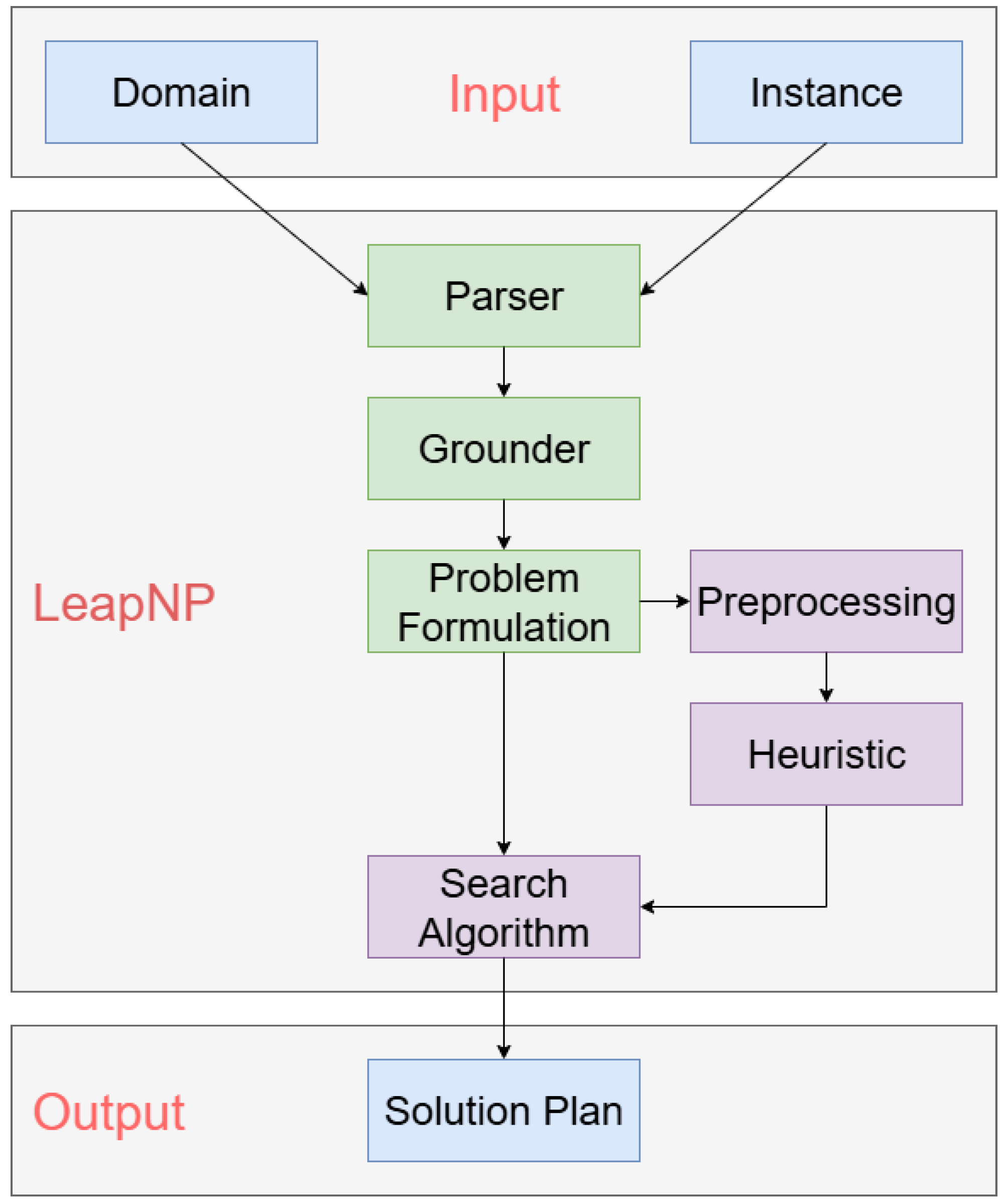
This section details the internal anatomy of LeapNP. The framework is built upon a strictly modular design philosophy: with the sole exception of the initial parsing module, every component operates as an independent unit that can be substituted without disrupting the overall pipeline. This approach ensures high customizability and architectural transparency as illustrated by the high-level schematic in Figure 1.

4.1. Parser and Grounder

The parser uses the PDDLReader defined in the Unified Planning framework [1], which reads the problem in PDDL format and parses it into a Unified Planning (UP) problem. Alternatively, it is also possible to use the problem directly in the UP format as input. Regarding the parsing stage, the framework natively handles classical, numeric, and temporal PDDL inputs. The subsequent grounding phase is responsible for transforming the lifted action schemas and problem objects into a fully grounded representation (see Figure 1). By default, LeapNP incorporates an adapter for the ENHSP grounding engine (https://github.com/hstairs/jpddlplus, accessed on 29 October 2025) integrated within the Unified Planning ecosystem. This configuration not only yields the grounded instance but also preserves a crucial traceback map that links concrete actions back to their original schemas. Crucially, this component is entirely swappable: users can seamlessly substitute the default engine with any other grounder supported by UP, or even integrate a proprietary solution by following the standard UP extension protocols.

4.2. Problem Formulation

Although the Unified Planning framework excels as a high-level abstraction layer for parsing and accessing diverse grounding engines, its internal architecture is primarily engineered for broad compatibility rather than execution speed. Its native data structures are designed to support a wide variety of planning techniques, resulting in a level of generalization that introduces unnecessary overhead during intensive search operations. To mitigate this, we implement a dedicated reformulation step. Immediately after grounding, the essential elements of the instance, specifically the initial state, goal conditions, and the set of grounded actions, are mapped into specialized, streamlined data structures. These custom representations are significantly lighter and optimized to facilitate rapid state manipulation within our search routines.

4.3. Preprocessing and Heuristic

Since different heuristics may rely on distinct preprocessing steps, our framework allows for flexible initialization. To implement a new heuristic, only two components are needed: an initialization routine (or preprocessing) to store any precomputed structure, and an evaluation function that maps a given state to a heuristic value for the search algorithm. The latter is the function that will be later used by the search algorithm.

4.4. Search Algorithm

The search engine operates by consuming two primary inputs: the planning problem generated by the formulation problem formulation module and the heuristic function used to assess state quality (see Figure 1). The framework is designed for maximum extensibility; researchers can introduce novel exploration strategies by simply inheriting from the abstract SearchAlgorithm base class and overriding the solve method with their custom logic. Upon successful termination, the algorithm yields the sequence of actions that constitutes the solution plan.

5. Modules

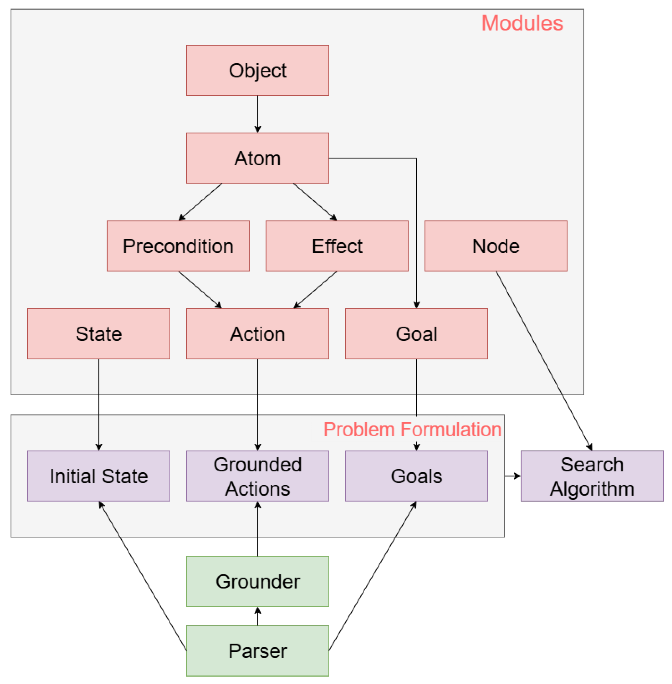
Figure 2 outlines the hierarchy of custom data structures implemented within our framework. These classes were engineered to digest the raw output from the UP library and re-instantiate the planning task into a more accessible format. Specifically, we focus on providing a streamlined interface for managing actions, goals, and state variables, particularly for domains involving complex numeric dependencies.

5.1. Object and Atom

The Object class constitutes the primitive layer of our data model. Its role is strictly to encapsulate the identity of domain entities, storing their unique designations and type hierarchies. These object instances subsequently serve as the arguments for instantiating actions and defining state variables.

Moving up the abstraction ladder, atoms encapsulate the grounded fluents of the planning task. These components act as the operative variables within the system, appearing ubiquitously in goal formulas, action preconditions, and effect lists. The module is engineered to offer a standardized API for querying and modifying values across different expression types. Specifically, every atom instance comprises:

• The name of the atom;
• The list of objects it involves;
• The name of the corresponding lifted fluent.

To manage numeric dynamics, the system employs a dynamic evaluation strategy. Arithmetic expressions are maintained as raw string templates; during the evaluation phase, the planner identifies any referenced atoms and injects their real-time values directly into the string. This modified formula is then processed by a lightweight mechanism. Although architecturally straightforward, this method ensures high flexibility, allowing the framework to support complex numeric modeling scenarios.

5.2. State and Node Representation

We distinguish between the physical configuration of the problem and the search context. A state captures the former: it is a static collection of fluent values describing the world at a specific instance, independent of how that configuration was achieved. The node structure, conversely, is designed to handle the exploration logic. It encapsulates the state instance and enriches it with the tracking data necessary to reconstruct the plan. The attributes stored in a node are:

• A dictionary mapping variable names to their current values (both Boolean and numeric);
• A unique identifier derived from a hash of the node’s variable values, used to avoid revisiting duplicates;
• The g value (cost from the initial state to the current state);
• The h value (heuristic estimate to the goal);
• A reference to the parent node;
• The action that generates the node from its parent.

The Node module provides comparison and hashing utilities to manage open and closed lists, as well as a method to expand a node by applying all applicable grounded actions and generating valid successors.

5.3. Action Encoding

The Action module represents grounded actions, each derived from an action schema instantiated with concrete objects. Actions include both preconditions and effects, which can be either Boolean or numeric. Each action object stores:

• A unique name (e.g., increment_c1);
• A list of preconditions;
• A list of effects.

Preconditions and effects are represented using their own dedicated modules:

• Precondition

• A name for the condition;
• A list of atoms (fluents) referenced;
• A flag indicating whether the condition is Boolean or numeric.
• A method to check the satisfaction of the condition in a given state.

• Effect

• A name for the effect.
• A list of involved atoms.
• A flag indicating whether the effect is Boolean or numeric.
• A left-hand side (a fluent).
• A right-hand side (a constant or expression).
• An operator (e.g., $=,+=,-=$) for numeric effects.
• A method to apply the effect to a given state.

Example 1 (Counters domain).

The objective of this numeric planning domain is to increase or decrease the value of the counters to achieve a particular configuration of such counters.

• Current State: $value\left(c_0\right)=0$, $value\left(c_1\right)=8$, $max\_int=8$.
• Goals: $value\left(c_0\right)+1\le value\left(c_1\right)$
• Atoms: $value\left(c_0\right),value\left(c_1\right)$.
• Constants: $max\_int$.
• Objects: counter $c_0,c_1$.
• Grounded Actions: $increment\_c_0,decrement\_c_0$, $increment\_c_1,decrement\_c_1$.
• Action Preconditions: $value(?c)-max\_int+1\le 0$, $1-value(?c)\le 0$.
• Action Effects: $value(?c)=value(?c)+1$, $value(?c)=value(?c)-1$.

When the search algorithm expands a new state, it first checks, for each grounded action, if the action is applicable in the current state. For the action $increment\_c_0$, the only precondition is $value\left(c_0\right)-max\_int+1\le 0$. $c_0$ is a constant; therefore, its value is already in the precondition, which becomes $value\left(c_0\right)-8+1\le 0$. Then, to evaluate if the precondition holds, it checks the list of atoms for the precondition, in this case only $value\left(c_0\right)$, it extracts its value from the current state, and the precondition becomes $0-8+1\le 0$. Then, the precondition is evaluated, and if it holds, the same process occurs for the action effects. The only effect of this action is $value\left(c_0\right)+1$, which again is evaluated, and the result is stored in the new state.

5.4. Goal Conditions

The Goal module defines the desired final conditions for the planning task. These are evaluated over a candidate state to determine whether it satisfies the problem objective. Each goal consists of:

• A string representing the goal expression;
• A list of referenced atoms;
• A Boolean flag distinguishing between Boolean and numeric goals;
• A method to verify goal satisfaction over a given state.

6. Search Algorithms, Structure and Techniques Implemented

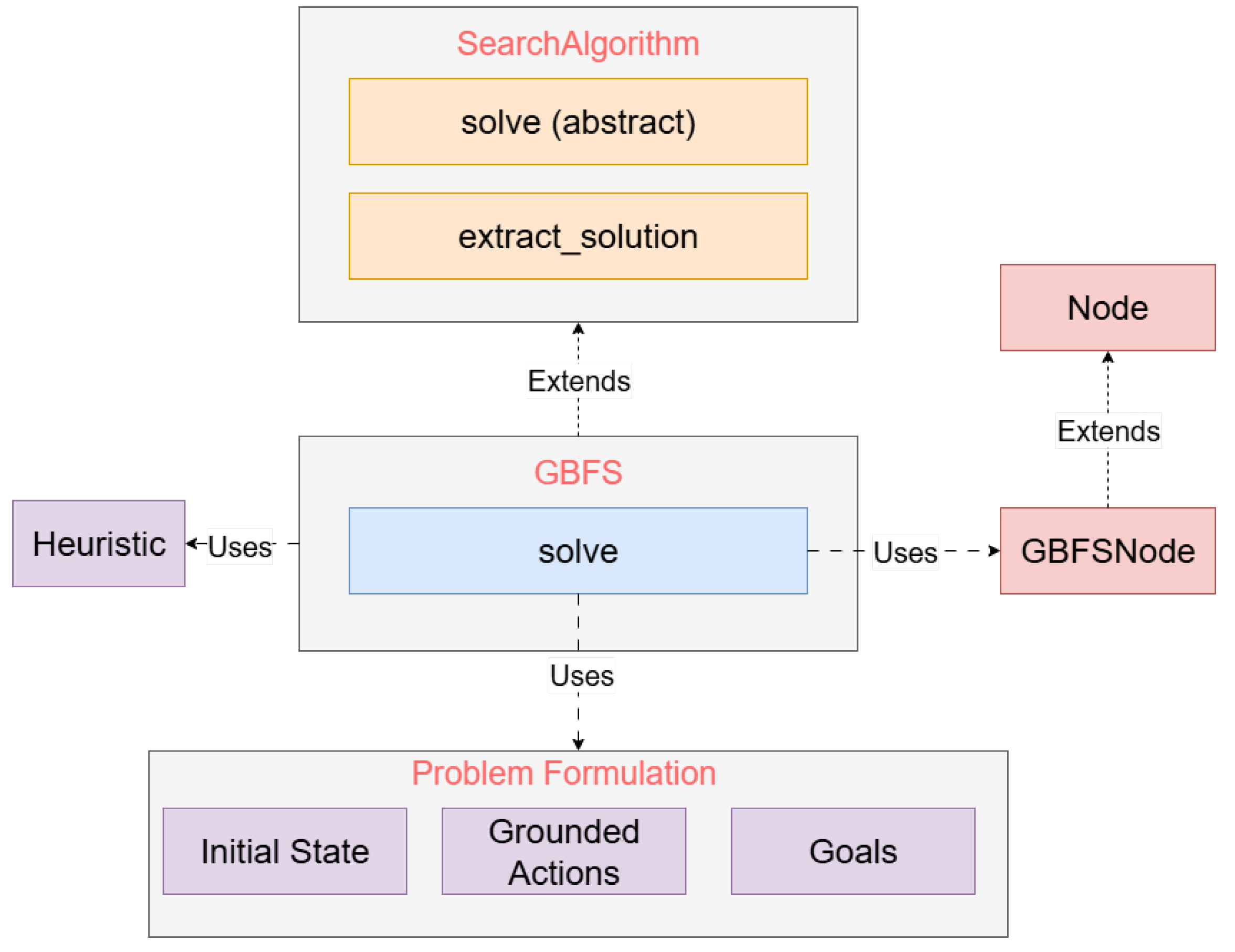
The backbone of the search module is the SearchAlgorithm abstract class. This component standardizes the execution of all solvers by encapsulating performance metrics, specifically, counters for expanded and evaluated states, alongside helper methods for plan reconstruction upon goal achievement. To implement a new strategy, users must extend this class and define the logic within the solve method. Furthermore, this process typically necessitates a specialization of the Node class. Extending the node structure is crucial, as it dictates the comparison criteria for sorting elements within the priority queue and governs the generation of the search neighborhood. An instance of this architecture applied to Greedy Best-First Search (GBFS) is illustrated in Figure 3.

Complementing the standard algorithms, we provide a multiple evaluation variant for every search strategy. The fundamental distinction lies in the heuristic inquiry phase: rather than processing successor states sequentially as they are instantiated, this mode aggregates them for simultaneous evaluation. While this parallelization offers limited benefits for classical analytical heuristics, it proves crucial for deep learning models. By exploiting the batch inference capabilities inherent in neural networks (and the underlying GPU hardware), this technique effectively amortizes the computational cost, resulting in a substantial reduction in total search time.

Traditional search algorithms (such as GBFS [3], A* [4], and WA* [31]), along with their multiple evaluation counterparts, manage the search space using two primary data structures. The priority queue contains the candidate states waiting to be expanded, sorted according to the comparison metric defined in the specific Node subclass (e.g., ascending h-values for GBFS). Simultaneously, the closed list serves as an archive for processed states. This structure fulfills a dual purpose: it prevents redundant computations by pruning cycles and stores the parent pointers necessary for reconstructing the final plan. To handle transpositions efficiently, the system enforces a strict update rule: if a previously evaluated state is encountered again via a new path, it is re-inserted into the priority queue only if the new trajectory offers a lower cost (g-value) than the one already existing in the closed list.

6.1. A*

The A* algorithm [4] is widely used for its ability to find optimal solutions, provided that the heuristic function is admissible. In our framework, we implement A* by extending the base SearchAlgorithm class. The corresponding node implementation overrides the comparison method to order the priority queue based on the f-value, defined as $f\left(n\right)=g\left(n\right)+h\left(n\right)$, where $g\left(n\right)$ is the cost accumulated from the initial state to the node n, and $h\left(n\right)$ is the heuristic estimate to the goal. While the optimality of A* is guaranteed only with admissible heuristics, a property that learning-based heuristics usually do not satisfy, the algorithm remains an integral part of the library, catering to scenarios where minimizing plan cost is prioritized over runtime performance, or where the learned heuristic is specifically trained to approximate optimal values.

We also include Weighted A* (WA*) [31]. This variant modifies the evaluation function to $f\left(n\right)=g\left(n\right)+w·h\left(n\right)$, with $w>1$. By inflating the heuristic influence, this parameter makes the search greedier, prioritizing nodes that appear closer to the goal over those with lower accumulated costs. This introduces a trade-off: it typically reduces the number of node expansions and runtime significantly, at the expense of solution optimality.

6.2. Greedy Best-First Search

Greedy Best-First Search (GBFS) [3] is a search strategy that prioritizes exploration based solely on the heuristic value $h\left(n\right)$. This approach typically leads to faster solutions compared to A*, albeit without guarantees on optimality, and in general with a worse quality of the found plans. The implementation of the algorithm using our modules can be seen in Figure 3. GBFS serves as the primary baselines for our experimental analysis, as our proposed variants are essentially parallelized extensions of this standard greedy approach.

6.3. Parallelism over Different States

The rationale behind our multiple evaluation strategy is grounded in the distinct computational nature of GNNs. While other deep learning architectures typically treat inputs as independent units, making parallelization straightforward, GNNs are constrained by the dense connectivity of the data. Since the computation for nodes and edges is intrinsically coupled through the graph structure, decomposing a single state for parallel execution is algorithmically complex. Consequently, seeking parallelism within a solitary instance is inefficient. What we can do instead is give as input multiple states: each state represents a graph that is independent from the others, achieving something similar to mini-batch parallelism (refer to [32] for additional information on this matter). In addition, one issue with mini-batch parallelism is the possibility of causing load imbalance when graphs have large differences in their dimension. In our case, our graphs are quite similar in their dimensions: the number of nodes represents the objects of the problem, and the different relations are fixed for the domain. There will be a difference in the number of edges among different instances, but not enough to cause a load imbalance.

Note that this type of parallelization is not new; it is a technique often used in general policies, in [28]. While not explicitly stated, it is used in their architecture. Our contribution relies on the idea of introducing this parallelism inside traditional search algorithms, such as GBFS, A* [4], and WA*, enabling more efficient exploration by evaluating multiple states simultaneously through a single GNN forward pass. This approach not only improves computational efficiency but also opens the door to integrating learned policies more tightly with our framework. We refer to these parallelized implementations as MBFS, MA*, and MWA*.

6.4. Deferred Multiple Evaluation

In the context of general policies, execution is typically memoryless: the algorithm greedily selects the most promising transition and immediately discards all alternative paths. Consequently, parallel computation is strictly limited to the expansion of the current state, as no other candidates are preserved. Unlike pure policy execution, our approach relies on a search-based exploration that naturally accumulates a buffer of unexpanded nodes. This structural difference enables us to implement a deferred evaluation strategy, where successors from distinct parent nodes are aggregated into a single, comprehensive batch. By decoupling expansion from evaluation, we achieve a much higher degree of parallelism, effectively leveraging the throughput capabilities of modern hardware.

The complete pseudocode is shown in Algorithm 1. The inputs are the initial state of the problem $s_0$, the set of grounded actions A, the goal of the problem G, and the heuristic function h. After the initialization (lines 1–2) and a goal satisfaction check (lines 4–6), the core logic diverges from standard GBFS in the expansion phase. Instead of evaluating successors immediately, the algorithm employs a two-stage collection process. First, the immediate successors of the current state s are generated and added to a temporary Batch container without being evaluated (lines 7–10). Subsequently, the algorithm iterates through these unevaluated successors to generate a second layer of states, which are collected in NewBatch (lines 11–15). In both cases, a state is added only if it has not been evaluated before (i.e., it must not be in the closed set), or if it has been evaluated with a higher accumulated cost g. Finally, the two sets are merged, and the heuristic values for all collected states are computed in a single ParallelEvaluate call, before putting them in the Open list (i.e., the priority queue) to order them (lines 16–18).

Our approach draws inspiration from deferred heuristic evaluation, a technique originally introduced in Fast Downward [33] as a variant of best-first search algorithms. In the original setting, successor states are not evaluated immediately; instead, they are added to the open list, inheriting their parent’s heuristic value. While the primary goal of this technique is to reduce the computational burden by skipping evaluations, we repurpose the mechanism with the opposite objective: we aim to maximize the number of evaluations performed in parallel. By deferring individual evaluations, we can accumulate a large set of successors from different parents, thereby enabling highly efficient, parallel GNN-based inference. This strategy allows us to process a broader set of promising states simultaneously, enhancing both the speed and coverage of the search while also reducing the risk of prematurely discarding potentially useful paths due to early local estimation errors. To implement this, we delay evaluation until the second generation of successors is produced. Instead of evaluating immediate successors, we proceed to expand their children, effectively advancing two levels into the search tree before performing any heuristic computation (Algorithm 1). Once this broader set of states is accumulated, we evaluate them concurrently in a single, parallel GNN forward pass.

Algorithm 1 Deferred Multiple Evaluation Best-First Search (DBFS)

Input: $\langle s_0,A,G\rangle$—initial state, list of grounded actions, and goal.   h—heuristic function.   Output: Solution plan from initial state to goal, or none. 1: $Open\leftarrow \left\{s_0\right\}$                    ▹priority queue ordered by h 2: $Closed\leftarrow \left\{s_0\right\}$ 3: while $Open\ne \varnothing$  do 4:       $s\leftarrow$ Pop($Open$)                     ▹state with lowest h 5:       if IsGoal($s,G$) then 6:             return ExtractSolution($s,Closed$) 7:       $Batch\leftarrow \varnothing$ 8:       for all $s^{\prime }\in$ Successors($s,A$) do 9:             if $s^{\prime }\notin Closed\vee g\left(s\right)+c(a,s)<g\left(s^{\prime }\right)$ then 10:                 $Closed\leftarrow Closed\cup \left\{s^{\prime }\right\};Batch\leftarrow Batch\cup \left\{s^{\prime }\right\}$ 11:     $NewBatch\leftarrow \varnothing$ 12:     for all $s^{\prime }\in Batch$ do 13:           for all $s^{″}\in$ Successors($s^{\prime },A$) do 14:                 if $s^{″}\notin Closed\vee g\left(s^{\prime }\right)+c(a,s^{\prime })<g\left(s^{″}\right)$ then 15:                      $Closed\leftarrow Closed\cup \left\{s^{″}\right\};NewBatch\leftarrow NewBatch\cup \left\{s^{″}\right\}$ 16:     $Batch\leftarrow Batch\cup NewBatch$ 17:     ParallelEvaluate($Batch,h$)                ▹single GPU call 18:     $Open\leftarrow Open\cup Batch$ 19: return  none

6.5. Greedy Search (General Policy)

In the literature of learning for planning, a heuristic function h defines a general policy if it can guide the agent to the goal greedily, without the need for backtracking or systematic search structures. As noted in Ståhlberg et al. [34], the heuristic does not have to be perfect.

Since several learning-based heuristics can be utilized as general policies, we also include a specific implementation designed to exploit this capability. We refer to this approach simply as Greedy Search.

Unlike traditional search algorithms, which maintain open and closed lists to manage the search frontier and the exploration, this algorithm operates as a pure greedy execution loop. At each step, it generates the successors of the current state, evaluates them using the heuristic (or the general policy, since it is technically the same in this case), and selects the best one as the next state, discarding the rest.

This algorithm serves as a more interesting test for the quality of the learned model: it verifies whether the learned heuristic can actually function as a robust policy capable of solving the problem without relying on the safety net offered by the backtracking mechanisms used in standard search algorithms.

7. Experimental Evaluation

The primary objective of our experiments is to assess how the framework handles different search strategies when paired with GNN-based heuristics. Specifically, we benchmark our proposed methods, Multiple Evaluation and Deferred Multiple Evaluation, against a standard GBFS baseline. To guarantee a fair comparison, every algorithm is tested within the same Python framework described before and utilizes the same GNN-based heuristic described in [30]. The details regarding the hyperparameters of the heuristic and its training procedure are in Appendix A of Appendix [30]. Ideally, we would have extended this validation to include other learning-based heuristics for numeric planning. However, the only currently available alternative [9] is tightly coupled with the Numeric Fast Downward planner, preventing its direct integration into our modular system.

As numeric planning problems, we select nine domains from the International Planning Competition (IPC) 2023 Numeric Track [35]: Counters, Fo-Counters, Sailing, Fo-Sailing, Mprime, Expedition, Hydropower, Farmland, Fo-Farmland. Each domain consists of 20 instances, with increasing difficulty scaling from the first instance to the last. In the selected IPC domains, actions have unit costs by definition. Consequently, the plan cost reported in our experiments is equivalent to the plan length. Experiments are run on a single Intel Xeon Gold 6140M (2.30GHz) core with a 5 min timeout for search and an NVIDIA v100 32GB GPU.

First, we examine the effectiveness of our multiple evaluation variant, which we call MBFS, against GBFS. From the results in

Table 1. Comparison between $GBFS$ and $MBFS$ in terms of coverage, average time (s), and evaluated states per second. Average time and evaluated states per second are evaluated only in the instances solved by both systems.

Domain	$\mathit{GBFS}$			$\mathit{MBFS}$
	Coverage	Time	Nodes/s	Coverage	Time	Nodes/s
Counters	8	41.7	22.24	10	2.53	369.13
Fo-Counters	6	8	18.6	8	0.86	172.82
Sailing	1	146.2	17.23	2	10.52	239.63
Fo-Sailing	8	70.4	66.7	8	33.17	209.59
Mprime	6	15	21.4	8	0.62	521.83
Expedition	6	45	18	6	9.39	81.63
Hydropower	8	8.2	18.49	9	3.72	33.03
Farmland	8	42.39	35.53	10	7.90	176.67
Fo-Farmland	12	65.87	34.45	15	5.24	427.35

, it emerges quite clearly that MBFS, when used with our GNN-based heuristic, is much faster than GBFS.

Then we evaluate MBFS against the deferred multiple evaluation variant, which we call DBFS. From the results in

Table 2. Comparison between $MBFS$ and $DBFS$ in terms of coverage, average time (s), evaluated states per second, and plan length. Average time, evaluated states per second, and plan length are evaluated only in the instances solved by both systems.

Domain	$\mathit{MBFS}$				$\mathit{DBFS}$
	Cov.	Time	Nodes/s	Plan Length	Cov.	Time	Nodes/s	Plan Length
Counters	10	13.89	464.5	100.3	10	28.96	708.3	89.4
Fo-Counters	8	32.98	170.3	22.0	7	1.66	717.5	15.1
Sailing	2	13.08	290.1	180.5	2	14.59	262.6	182.5
Fo-Sailing	8	33.17	209.6	269.6	8	70.47	667.2	231.5
Mprime	8	1.42	630.2	10.2	8	34.07	812.8	12.9
Expedition	6	9.40	81.6	103.7	8	11.49	188.1	165.3
Hydropower	9	6.90	29.3	38.6	9	8.11	55.0	38.8
Farmland	10	19.98	241.2	250.9	13	7.23	786.2	246.0
Fo-Farmland	15	5.74	419.3	174.5	13	2.31	1409.3	51.3

, DBFS consistently evaluates many more nodes per second compared to MBFS; this does not necessarily translate into better performance. Although DBFS achieves slightly higher overall coverage and allows for the exploration of states that would otherwise be skipped; this comes at a cost: the additional evaluations lead to higher average runtimes in 6 of the 9 domains, without a clear improvement in plan quality. In other words, the ability to evaluate more nodes does not always correspond to more efficient or effective search behavior; additionally, DBFS is much more expensive in terms of GPU memory usage.

In Table 3, we show the memory allocated for GBFS, MBFS, and DBFS for the most difficult instance of each of the considered domains; we can identify three different groups of domains, based on their branching factor. The branching factor is the medium number of applicable actions in a set of states. It can be formally defined as

$$b={\displaystyle \frac{1}{\left|S\right|}}\sum _{s\in S}\left|A\left(s\right)\right|$$

(1)

where

• b is the branching factor;
• S is the set of considered states;
• $A\left(s\right)$ is the set of applicable actions in state s;
• $|·|$ denotes the cardinality of a set.

Table 3. GPU memory usage (in MB) comparison of GBFS, MBFS and DBFS for the most difficult instance of each domain.

Domain	$\mathit{GBFS}$	$\mathit{MBFS}$	$\mathit{DBFS}$
Expedition	659	677	765
Hydropower	667	685	767
Farmland	659	662	699
Fo-Farmland	657	659	811
Sailing	667	989	5015
Fo-Sailing	661	871	5959
Counters	663	1265	23,200
Fo-Counters	661	1265	24,687
Mprime	665	4861	>32,000

Table 3. GPU memory usage (in MB) comparison of GBFS, MBFS and DBFS for the most difficult instance of each domain.

Domain	$\mathit{GBFS}$	$\mathit{MBFS}$	$\mathit{DBFS}$
Expedition	659	677	765
Hydropower	667	685	767
Farmland	659	662	699
Fo-Farmland	657	659	811
Sailing	667	989	5015
Fo-Sailing	661	871	5959
Counters	663	1265	23,200
Fo-Counters	661	1265	24,687
Mprime	665	4861	>32,000

Therefore, we can identify the domains where even the hardest instances exhibit a low branching factor (Expedition, Hydropower, Farmland, and Fo-Farmland), domains exhibiting an intermediate branching factor (Sailing and Fo-Sailing), and domains with a high branching factor in the hardest instances Counters, Fo-Counters, and Mprime). For the first group, we can see that the differences in memory usage are minimal among the three variants; in those domains, the memory required to store the learned weights of the model is much higher than the memory required to store the graph representing the different states. In the second group, we observe that the memory usage for MBFS increases slightly, whereas for DBFS it already reaches values exceeding 5GB. Finally, in the third group, for Counters and Fo-Counters, memory consumption already increases with MBFS, although it remains within reasonable limits. In contrast, for Mprime, the domain characterized by the highest branching factor among those analyzed, memory usage approaches 5 GB already with MBFS, and DBFS quickly saturates the available memory.

7.1. Optimization vs. Speed

While MBFS focuses on finding a solution as quickly as possible by aggressively following the heuristic gradient, many real-world applications require minimizing the cost of the plan. To support this, LeapNP also implements MA* (multiple evaluation A*), a batch-aware implementation of the A* algorithm. Like MBFS, MA* evaluates successors in parallel to maximize GPU throughput.

Table 4. Comparison between $MBFS$ and MA* in terms of coverage, average time (s), and plan length. Average time and plan length are evaluated only in the instances solved by both systems.

Domain	$\mathit{MBFS}$			MA*
	Coverage	Time	Plan Length	Coverage	Time	Plan Length
Counters	10	0.94	18.0	5	44.43	18.0
Fo-Counters	8	0.53	7.3	4	3.22	7.3
Sailing	2	-	-	0	-	-
Fo-Sailing	8	5.74	67.5	2	117.01	65.5
Mprime	8	1.42	10.3	9	31.77	6.8
Expedition	6	2.82	52.0	4	7.73	52.0
Hydropower	9	2.38	35.0	5	20.29	34.8
Farmland	10	10.18	221.4	7	62.41	211.4
Fo-Farmland	15	5.68	177.1	11	29.76	28.8

compares the performance of MBFS against MA*. Interestingly, the results show that in the majority of the tested domains, MBFS produces plans with costs identical or very close to those found by MA*. This finding highlights the high informativeness of the learned heuristics, which can often find near-optimal paths, minimizing the need for extensive exploration. The only two notable exceptions are Mprime and Fo-Farmland, where MA* finds significantly better solutions. In terms of computational costs, MA* naturally pays a price in runtime and coverage compared to MBFS, as it requires exploring a larger portion of the state space.

In Appendix B of the appendix, we show that our Python-based planner, when equipped with our learning-based heuristic, achieves performance competitive with state-of-the-art numeric planners, despite the inherent overhead of an interpreted language. We show the comparison with the ENHSP planning system, which uses the state-of-the-art traditional heuristic $h^{mrp}$ [36], and with the only other learning-based heuristic for numeric planning, $h_{rank}^{ccWLF}$ [9], implemented in Numeric Fast Downward.

7.2. Search vs. Policy

In this final analysis, we investigate the intrinsic quality of the learned heuristics by stripping away the search mechanism. We compare MBFS against a pure Greedy Search. The Greedy Search approach treats the heuristic as a general policy: at each step, it generates successors, evaluates them in a single batch, and deterministically selects the best one, discarding the rest.

Table 5. Comparison between MBFS and GreedySearch in terms of coverage, average time (s), and plan length. Average time and plan length are evaluated only in the instances solved by both systems.

Domain	$\mathit{MBFS}$			$\mathit{GreedySearch}$
	Coverage	Time	Plan Length	Coverage	Time	Plan Length
Counters	10	2.53	49.3	8	14.47	280.8
Fo-Counters	8	32.98	22.0	7	1.15	14.3
Sailing	2	13.08	180.5	2	14.51	182.0
Fo-Sailing	8	33.17	269.6	8	29.99	269.5
Mprime	8	1.49	10.1	7	0.65	6.6
Expedition	6	2.82	52.0	4	2.81	52.0
Hydropower	9	2.78	42.5	2	2.65	42.5
Farmland	10	7.59	302.7	3	7.26	302.7
Fo-Farmland	15	6.13	190.7	9	7.31	214.9

shows the comparison between MBFS and Greedy Search. The gap in the coverage between MBFS and Greedy Search reveals the “imperfections” of the learned heuristics. We can observe that in Fo-Counters, Sailing and Fo-Sailing, both the coverage and plan length remain strictly comparable. This indicates that the instances solved in these domains do not rely on the backtracking capabilities of MBFS but depend almost exclusively on the accurate guidance provided by the learned heuristics. Conversely, on the other domains, the significant drop in coverage for Greedy Search highlights scenarios where the heuristics provide misleading guidance or lead to dead ends. In these cases, the systematic search structure of MBFS proves essential, acting as a safety net to recover from heuristic errors and escape search plateaus that a pure policy-based approach cannot overcome.

8. Conclusions

In this work, we introduced a fully Python-based planning framework tailored for the integration and evaluation of learning-based heuristics, with a specific focus on numeric planning problems. LeapNP is modular, lightweight, and designed to support rapid experimentation with deep learning models, particularly GNNs. This flexibility enables researchers to easily implement and test custom heuristics and search strategies without the overhead commonly associated with traditional planners. By doing so, this platform creates a fertile ground for innovation in learning-based planning. It is our sincere hope that LeapNP serves as a valuable asset for the research community, empowering scholars to tackle these complex challenges in a more accessible and straightforward manner.

Leveraging this flexible architecture, we introduced two variants of standard search algorithms: Multiple Evaluation Best-First Search (MBFS) and Deferred Multiple Evaluation Best-First Search (DBFS). Both methods were designed to maximize the efficiency of GNN-based heuristics by leveraging parallelism and batch evaluation. Our experiments on the IPC 2023 numeric planning benchmark suite demonstrate that MBFS significantly improves evaluation speed compared to standard GBFS, particularly in domains with high branching factors. While DBFS successfully achieves even higher evaluation throughput by deferring and batching evaluations across multiple parents, our analysis reveals that this metric does not necessarily translate to better search performance. In practice, DBFS tends to incur higher runtimes and substantial memory overhead, especially in domains with high branching factors, without delivering consistent improvements in plan quality or coverage. These findings indicate that while the core premise of parallel state expansion is promising, the current implementation, based on the indiscriminate collection of second-generation successors, may be suboptimal. To fully unlock the potential of deferred multiple evaluation, a more sophisticated selection mechanism is likely required. Future work will therefore focus on exploring refined, adaptive batching strategies that can balance throughput with search direction quality.

Beyond standard satisficing search, our analysis extended to the two extremes of the planning spectrum: cost-optimal reasoning and pure policy execution. On one hand, the comparison with MA* revealed the high quality of the learned heuristic: in most domains, they successfully guided the greedy MBFS towards near-optimal solutions, effectively minimizing the need for exhaustive search. However, exceptions such as Mprime and Fo-Farmland highlighted that for specific complex problems, the systematic exploration of MA* remains essential to uncover significantly better plans that aggressive greedy strategies miss. On the other hand, our Greedy Search mode allowed us to isolate the policy component to assess the intrinsic robustness of these models as standalone general policies. By removing the safety net of backtracking, we were able to distinguish when the heuristic merely offers guidance and when it was capable of solving complex instances “execution-style”, identifying exactly where the underlying search algorithm is needed to compensate for prediction errors.

Ultimately, LeapNP is designed as a comprehensive framework and benchmarking suite. By providing a diverse set of algorithms, ranging from high-throughput satisficing search (MBFS and DBFS) to cost-sensitive (MA*) and policy-based execution (Greedy Search), we allow researchers to dissect and have a deeper insight into the trade-offs of their learned heuristics, in order to better understand how learning components interact with symbolic search.

8.1. Potential Applications in Network Orchestration

While our experimental evaluation focuses on standard IPC benchmarks, the architecture of LeapNP is particularly suited to address the offline resource orchestration challenges typical of Software-Defined Networking (SDN) and Service-Oriented Architectures. Unlike packet-level processing, which requires nanosecond latency, orchestration tasks, such as the periodic re-optimization of Service Function Chains (SFCs) or penetration testing simulation, are computationally intensive planning problems where solution quality and constraint satisfaction prioritize raw execution speed.

• Handling Complex Numeric Constraints: As discussed in the background, modern networks impose strict numeric constraints on Quality of Service (QoS) metrics like bandwidth and latency. The LeapNP native support for numeric fluents allows researchers to model these resource limits directly. Unlike static solvers, LeapNP enables the prototyping of learning-based heuristics that can navigate these highly constrained numeric state spaces more effectively, finding feasible configurations for SFC placement where manual scripting often fails.
• Generalization via GNNs: Network topologies are dynamic but often share structural substructures. The LeapNP native support for GNNs allows for the training of heuristics that generalize across different network sizes and topologies. This is particularly valuable for SFC, where a policy learned on a small testbed can be transferred to larger, real-world network instances without retraining.

8.2. Limitations

While LeapNP provides a highly modular and accessible environment for research, users should be aware of two primary limitations when applying it to practical problems:

• Language-Specific Performance Overhead: Since the framework is implemented entirely in Python, it prioritizes clarity and modifiability over raw execution speed. Consequently, when used with traditional, non-neural heuristics, LeapNP is inevitably slower in terms of nodes expanded per second compared to state-of-the-art planners written in low-level languages like C++ or Java. This framework is intended for rapid prototyping and research at the intersection of deep learning and planning, rather than for production environments requiring maximum search speed.
• Memory Constraints in High-Branching Domains: The parallel evaluation variants (MBFS, DBFS, and MA*) rely on batching multiple states into single GPU forward passes. Our experiments show that in domains with a high branching factor, such as Mprime or Counters, the memory required to store and process these batches can grow significantly. For very large instances or hardware with limited GPU memory, this can lead to memory saturation, acting as a physical constraint on the search depth and batch size.

References

- Micheli, A.; Bit-Monnot, A.; Röger, G.; Scala, E.; Valentini, A.; Framba, L.; Rovetta, A.; Trapasso, A.; Bonassi, L.; Gerevini, A.E.; et al. Unified Planning: Modeling, manipulating and solving AI planning problems in Python. SoftwareX 2025, 29, 102012. [Google Scholar] [CrossRef]
- Alkhazraji, Y.; Frorath, M.; Grützner, M.; Helmert, M.; Liebetraut, T.; Mattmüller, R.; Ortlieb, M.; Seipp, J.; Springenberg, T.; Stahl, P.; et al. Pyperplan, Version v1.3. 2020. Available online: https://zenodo.org/records/3701399 (accessed on 29 October 2025).
- Bonet, B.; Geffner, H. Planning as heuristic search. Artif. Intell. 2001, 129, 5–33. [Google Scholar] [CrossRef]
- Hart, P.E.; Nilsson, N.J.; Raphael, B. A formal basis for the heuristic determination of minimum cost paths. IEEE Trans. Syst. Sci. Cybern. 1968, 4, 100–107. [Google Scholar] [CrossRef]
- Borelli, V.; Gerevini, A.E.; Scala, E.; Serina, I. Modular Numeric Planning in Python: A Framework for Learning-Based Heuristics. In Proceedings of the International Conference on Data Science and Emerging Technologies; Springer: Berlin/Heidelberg, Germany, 2025. [Google Scholar]
- Helmert, M. The fast downward planning system. J. Artif. Intell. Res. 2006, 26, 191–246. [Google Scholar] [CrossRef]
- Aldinger, J.; Nebel, B. Interval based relaxation heuristics for numeric planning with action costs. In Proceedings of the Joint German/Austrian Conference on Artificial Intelligence (Künstliche Intelligenz); Springer: Berlin/Heidelberg, Germany, 2017; pp. 15–28. [Google Scholar]
- Chen, D.Z.; Trevizan, F.; Thiébaux, S. Return to Tradition: Learning Reliable Heuristics with Classical Machine Learning. In Proceedings of the International Conference on Automated Planning and Scheduling, Banff, AL, Canada, 1–6 June 2024; Volume 34, pp. 68–76. [Google Scholar]
- Chen, D.; Thiébaux, S. Graph learning for numeric planning. Adv. Neural Inf. Process. Syst. 2024, 37, 91156–91183. [Google Scholar]
- Ferber, P.; Helmert, M.; Hoffmann, J. Neural network heuristics for classical planning: A study of hyperparameter space. In ECAI 2020; IOS Press: Amsterdam, The Netherlands, 2020; pp. 2346–2353. [Google Scholar]
- Scala, E.; Haslum, P.; Thiébaux, S.; Ramírez, M. Subgoaling Techniques for Satisficing and Optimal Numeric Planning. J. Artif. Intell. Res. 2020, 68, 691–752. [Google Scholar] [CrossRef]
- Shen, W.; Trevizan, F.; Thiébaux, S. Learning domain-independent planning heuristics with hypergraph networks. In Proceedings of the International Conference on Automated Planning and Scheduling, Online, 19–30 October 2020; Volume 30, pp. 574–584. [Google Scholar]
- Karia, R.; Srivastava, S. Learning generalized relational heuristic networks for model-agnostic planning. In Proceedings of the AAAI Conference on Artificial Intelligence, Online, 2–9 February 2021; Volume 35, pp. 8064–8073. [Google Scholar]
- Corrêa, A.B.; Pereira, A.G.; Seipp, J. Classical Planning with LLM-Generated Heuristics: Challenging the State of the Art with Python Code. arXiv 2025, arXiv:2503.18809. [Google Scholar] [CrossRef]
- Piotrowski, W.; Perez, A.; Grover, S. Nyx: Planning for Emerging Problems with PDDL+ and Beyond. arXiv 2024, arXiv:2402.11901. [Google Scholar]
- Fox, M.; Long, D. PDDL+: Modeling continuous time dependent effects. In Proceedings of the 3rd International NASA Workshop on Planning and Scheduling for Space, Houston, TX, USA, 27–29 October 2002; Volume 4, p. 34. [Google Scholar]
- Vallati, M.; Magazzeni, D.; De Schutter, B.; Chrpa, L.; McCluskey, T. Efficient macroscopic urban traffic models for reducing congestion: A PDDL+ planning approach. In Proceedings of the AAAI Conference on Artificial Intelligence, Phoenix, AZ, USA, 12–17 February 2016; Volume 30. [Google Scholar]
- Doria, F.; Percassi, F.; Maratea, M.; Vallati, M. A Domain-specific Heuristic for PDDL+-based Traffic Signal Optimisation. In Proceedings of the 40th Annual AAAI Conference on Artificial Intelligence, Philadelphia, PA, USA, 25 February–4 March 2025; AAAI Press: Palo Alto, CA, USA, 2025. [Google Scholar]
- Cashmore, M.; Fox, M.; Long, D.; Magazzeni, D.; Ridder, B.; Carrera, A.; Palomeras, N.; Hurtos, N.; Carreras, M. Rosplan: Planning in the robot operating system. In Proceedings of the International Conference on Automated Planning and Scheduling, Jerusalem, Israel, 7–11 June 2015; Volume 25, pp. 333–341. [Google Scholar]
- Guo, H.; Wu, F.; Qin, Y.; Li, R.; Li, K.; Li, K. Recent trends in task and motion planning for robotics: A survey. ACM Comput. Surv. 2023, 55, 1–36. [Google Scholar] [CrossRef]
- Alaboud, F.K.; Coles, A. Personalized medication and activity planning in PDDL+. In Proceedings of the International Conference on Automated Planning and Scheduling, Berkeley, CA, USA, 11–15 July 2019; Volume 29, pp. 492–500. [Google Scholar]
- Chen, Z.; Kang, F.; Xiong, X.; Shu, H. A survey on penetration path planning in automated penetration testing. Appl. Sci. 2024, 14, 8355. [Google Scholar] [CrossRef]
- Naseri, M.; Towhidi, A. Qos-aware automatic composition of web services using ai planners. In Proceedings of the Second International Conference on Internet and Web Applications and Services (ICIW’07), Le Morne, Mauritius, 13–19 May 2007; IEEE: Piscataway, NJ, USA, 2007; p. 29-29. [Google Scholar]
- Mohamed, R.; Avgeris, M.; Leivadeas, A.; Lambadaris, I.; Chinneck, J.; Morris, T.; Djukic, P. Service function chain network planning through offline, online and infeasibility restoration techniques. Comput. Netw. 2024, 242, 110241. [Google Scholar] [CrossRef]
- Haslum, P.; Lipovetzky, N.; Magazzeni, D.; Muise, C. An Introduction to the Planning Domain Definition Language. In Synthesis Lectures on Artificial Intelligence and Machine Learning; Morgan & Claypool Publishers: San Rafael, CA, USA, 2019. [Google Scholar] [CrossRef]
- Fox, M.; Long, D. PDDL2.1: An Extension to PDDL for Expressing Temporal Planning Domains. J. Artif. Intell. Res. 2003, 20, 61–124. [Google Scholar] [CrossRef]
- Toyer, S.; Trevizan, F.; Thiébaux, S.; Xie, L. Action schema networks: Generalised policies with deep learning. In Proceedings of the AAAI Conference on Artificial Intelligence, New Orleans, LO, USA, 2–7 February 2018; Volume 32. [Google Scholar]
- Ståhlberg, S.; Bonet, B.; Geffner, H. Learning general optimal policies with graph neural networks: Expressive power, transparency, and limits. In Proceedings of the International Conference on Automated Planning and Scheduling, Online, 13–24 June 2022; Volume 32, pp. 629–637. [Google Scholar]
- Wang, R.X.; Thiébaux, S. Learning Generalised Policies for Numeric Planning. In Proceedings of the International Conference on Automated Planning and Scheduling, Banff, AL, Canada, 1–6 June 2024; Volume 34, pp. 633–642. [Google Scholar]
- Borelli, V.; Gerevini, A.E.; Scala, E.; Serina, I. Learning Heuristic Functions with Graph Neural Networks for Numeric Planning. In Proceedings of the AAAI Conference on Artificial Intelligence, Singapore, 20–27 January 2026; Volume 40. [Google Scholar]
- Ebendt, R.; Drechsler, R. Weighted A* search–unifying view and application. Artif. Intell. 2009, 173, 1310–1342. [Google Scholar] [CrossRef]
- Besta, M.; Hoefler, T. Parallel and distributed graph neural networks: An in-depth concurrency analysis. IEEE Trans. Pattern Anal. Mach. Intell. 2024, 46, 2584–2606. [Google Scholar] [CrossRef] [PubMed]
- Richter, S.; Helmert, M. Preferred operators and deferred evaluation in satisficing planning. In Proceedings of the International Conference on Automated Planning and Scheduling, Thessaloniki, Greece, 19–23 September 2009; Volume 19, pp. 273–280. [Google Scholar]
- Ståhlberg, S.; Bonet, B.; Geffner, H. Learning Generalized Policies without Supervision Using GNNs. In Proceedings of the International Conference on Principles of Knowledge Representation and Reasoning, Haifa, Israel, 31 July–5 August 2022; Volume 19, pp. 474–483. [Google Scholar]
- Taitler, A.; Alford, R.; Espasa, J.; Behnke, G.; Fiser, D.; Gimelfarb, M.; Pommerening, F.; Sanner, S.; Scala, E.; Schreiber, D.; et al. The 2023 International Planning Competition. AI Mag. 2024, 45, 280–296. [Google Scholar] [CrossRef]
- Scala, E.; Saetti, A.; Serina, I.; Gerevini, A.E. Search-Guidance Mechanisms for Numeric Planning Through Subgoaling Relaxation. In Proceedings of the Thirtieth International Conference on Automated Planning and Scheduling, Nancy, France, 26–30 October 2020; Beck, J.C., Buffet, O., Hoffmann, J., Karpas, E., Sohrabi, S., Eds.; AAAI Press: Palo Alto, CA, USA, 2020; pp. 226–234. [Google Scholar]
- Hamilton, W.L. Graph Representation Learning; Morgan & Claypool Publishers: San Rafael, CA, USA, 2020. [Google Scholar]