A Multi-Objective Optimization-Based Container Cloud Resource Scheduling Method

Abstract

Container-based cloud platforms enable flexible and lightweight application deployment, yet container scheduling remains challenged by resource fragmentation, load imbalance, excessive energy consumption, and service-level agreement (SLA) violations. To address these issues, this paper proposes a hybrid multi-objective optimization approach, termed HHO-GWO, which combines Harris Hawks Optimization (HHO) with the Grey Wolf Optimizer (GWO) for container initial placement in cloud environments. A unified fitness function is designed to jointly consider resource utilization, load balancing, resource fragmentation, energy consumption, and SLA violation rate. In addition, a dynamic weight adjustment mechanism and Lévy flight perturbation are incorporated to improve search adaptability and prevent premature convergence. The proposed method is evaluated through extensive simulations under different workload scales and compared with several representative metaheuristic algorithms. The results show that HHO-GWO achieves improved convergence behavior, solution quality, and stability, particularly in large-scale container deployment scenarios. These findings suggest that the proposed approach provides a practical and energy-aware solution for multi-objective container scheduling in cloud data centers.

1. Introduction

Cloud computing has become a fundamental paradigm for delivering on-demand computing resources and services over the Internet, enabling flexible and scalable resource provisioning for a wide range of applications [1,2,3]. With the rapid growth of data-intensive and latency-sensitive workloads, such as Internet of Things (IoT) applications, real-time data analytics, and large-scale online services, cloud platforms are required to manage increasingly dynamic and heterogeneous resource demands efficiently [4,5]. This rapid expansion of cloud workloads has further intensified the need for efficient resource scheduling and management mechanisms.

In recent years, microservice architecture has gained widespread adoption as an effective approach to building scalable and maintainable cloud applications. By decomposing monolithic applications into loosely coupled and independently deployable services, microservices significantly improve system flexibility and fault isolation [6,7]. Container virtualization has emerged as a key enabling technology for microservice-based systems due to its lightweight nature, fast startup time, and efficient resource isolation compared with traditional virtual machines [7,8]. As a result, container-based cloud platforms have been widely deployed in both centralized cloud data centers and hybrid cloud–edge environments [5,9].

Efficient container scheduling plays a crucial role in determining the overall performance of containerized cloud systems. Container scheduling typically involves assigning containers or tasks to physical hosts while satisfying resource constraints and optimizing system-level objectives such as load balancing, energy efficiency, and service quality [10,11]. Numerous scheduling strategies have been proposed to improve container performance from different perspectives. For instance, locality-aware scheduling approaches exploit data or service locality to reduce communication overhead [12], while prediction-driven scheduling methods leverage workload forecasting to improve scheduling decisions under dynamic workloads [13].

Despite these advances, container scheduling in practical cloud environments remains challenging [14]. Most existing scheduling strategies implicitly assume that computing resources on a physical host can be evenly or continuously shared among co-located containers. However, in real-world systems, resource demands are often uneven and time-varying, which may lead to inefficient resource utilization and load imbalance. In particular, suboptimal scheduling decisions can result in resource fragmentation, where available resources are distributed across hosts in small, non-contiguous portions that cannot be effectively allocated to incoming containers, even when sufficient aggregate capacity exists [7,15,16].

Resource fragmentation becomes especially problematic under high system load, as fragmented CPU or memory resources limit the ability of the scheduler to place new containers efficiently, leading to increased task response time and degraded system performance [17]. Moreover, fragmentation may exacerbate load imbalance across physical hosts, reducing the effectiveness of scheduling strategies that focus solely on aggregate resource metrics rather than resource continuity. Therefore, addressing load balancing and resource utilization in a unified manner is essential for improving the efficiency and robustness of container-based cloud systems [18].

To address the aforementioned challenges, this paper proposes a hybrid multi-objective container scheduling approach for cloud environments by integrating HHO and GWO. A unified fitness function is constructed to jointly consider resource utilization, load balancing, resource fragmentation, energy consumption, and SLA violations. Furthermore, a dynamic weight adjustment mechanism is introduced to balance global exploration and local exploitation during the optimization process, while Lévy flight perturbation is incorporated to enhance population diversity and avoid premature convergence. Extensive experiments, including ablation studies and comparative evaluations under different workload scales, are conducted to validate the effectiveness, convergence behavior, and robustness of the proposed method. The main contributions of this paper are as follows:

• A unified multi-objective container scheduling model is formulated for cloud environments, which jointly considers resource wastage, load balancing, resource fragmentation, energy consumption, and SLA violation within a single optimization framework, enabling coordinated optimization of conflicting objectives.
• A hybrid HHO–GWO scheduling algorithm is proposed by integrating the global guidance mechanism of the GWO with the strong local exploitation capability of HHO, achieving a balanced exploration–exploitation trade-off for large-scale container placement problems.
• Several enhancement mechanisms are incorporated, including dynamic weight adjustment, an improved escape energy decay strategy, Lévy flight perturbation, and pheromone-guided search, which effectively improve population diversity, convergence stability, and the ability to escape local optima.
• Extensive experimental evaluations and ablation studies under different workload scales demonstrate that the proposed method consistently outperforms several representative metaheuristic algorithms in terms of convergence speed, solution quality, and robustness.

Unlike existing hybrid metaheuristic schedulers that mainly rely on static parameter settings or loosely coupled hybridization strategies, the proposed HHO–GWO framework introduces a dynamically weighted cooperation mechanism between HHO and GWO. By jointly integrating adaptive escape energy control and Lévy flight perturbation, the proposed approach achieves a more balanced exploration–exploitation trade-off for container scheduling in cloud environments.

The remainder of this paper is organized as follows: Section 2 presents the system model and multi-objective optimization formulation. Section 3 introduces the proposed hybrid optimization algorithm. Section 4 describes the algorithm workflow and implementation details. Section 5 reports experimental results and performance analysis, followed by conclusions in Section 6.

2. Related Work

A wide range of container placement and scheduling approaches have been proposed in recent years to improve resource utilization, load balancing, and overall system performance in cloud environments. Multi-objective optimization has become a prominent research direction for addressing the conflicting goals inherent in container scheduling. Khan et al. proposed multi-objective container placement strategies for Container-as-a-Service (CaaS) platforms using evolutionary optimization techniques, demonstrating effective trade-offs among multiple performance objectives [9,19]. Genetic and evolutionary computation methods have also been applied to online container placement in heterogeneous clusters, improving adaptability and robustness under dynamic workloads [20,21]. These studies indicate that multi-objective formulations are effective in capturing the complexity of container scheduling problems; however, they often focus primarily on placement optimization and pay limited attention to resource fragmentation.

Metaheuristic algorithms have been widely adopted to further enhance container scheduling and load balancing performance due to their strong global search capability and flexibility in handling complex constraints. Nature-inspired optimization methods, such as Whale Optimization and GWO, have demonstrated promising results in reducing energy consumption and improving load distribution in cloud environments [22]. In addition, joint optimization strategies that simultaneously consider load balancing and resource allocation have been proposed for multi-cloud scenarios, achieving improved system efficiency and reliability [15,17]. Despite their effectiveness, metaheuristic-based approaches often require careful parameter tuning and may incur significant computational overhead in large-scale or highly dynamic cloud systems.

With the increasing complexity and dynamism of cloud environments, learning-based scheduling methods have attracted growing attention in recent years. Liu et al. in [23] proposed a multi-factorial evolutionary algorithm (MFEA) that evolves multiple optimization problems simultaneously for container placement in heterogeneous cluster environments. Wu et al. in [24] proposed Blender, a container placement strategy that leverages Zipf-like traffic distributions to reduce inter-container communication and improve load balancing across physical machines. Al-Moalmi et al. in [25] proposed a whale optimization system for energy-efficient container placement, aiming to minimize power consumption while maximizing resource utilization in heterogeneous cloud data center environments. Deep reinforcement learning has been applied to container placement and scheduling to learn adaptive policies based on system feedback, enabling improved resource utilization and decision quality [26,27]. Multi-agent reinforcement learning has further been explored to address large-scale resource allocation problems in container-based cloud environments, enhancing scalability through decentralized decision-making [28]. Moreover, learning-based approaches have been extended to edge computing and microservice deployment scenarios by incorporating structural information to improve scheduling effectiveness [25,29]. Although these methods show strong adaptability, they typically require extensive training data and computational resources, which may limit their practical applicability.

Overall, existing research has achieved significant progress in container placement and scheduling through multi-objective optimization, metaheuristic algorithms, and learning-based approaches. However, most studies treat container placement and task scheduling as separate problems and do not explicitly consider the joint impact of load balancing and resource fragmentation. This limitation becomes particularly critical under high-load conditions, motivating the need for resource-aware scheduling strategies that can better exploit available resources in container-based cloud environments.

3. System Model and Problem Formulation

3.1. Problem Description

The scheduling decisions made during the initial deployment stage of containers have a significant impact on subsequent system performance, resource utilization efficiency, and energy consumption. To achieve intelligent and efficient container resource scheduling, it is essential to construct a well-designed optimization model that comprehensively captures the multi-dimensional constraints and performance objectives encountered in practical deployment scenarios.

In this chapter, the container scheduling problem is first formally described to clarify the problem context and fundamental assumptions. Subsequently, based on the resource characteristics of containers and physical hosts, a multi-objective optimization model is developed. The model jointly considers five key dimensions, namely resource utilization, load balancing, resource fragmentation, energy consumption, and SLA satisfaction, and integrates them into a comprehensive fitness function. Furthermore, a dynamic weighting mechanism is introduced to enhance the adaptability and optimization effectiveness of the model across different scheduling stages.

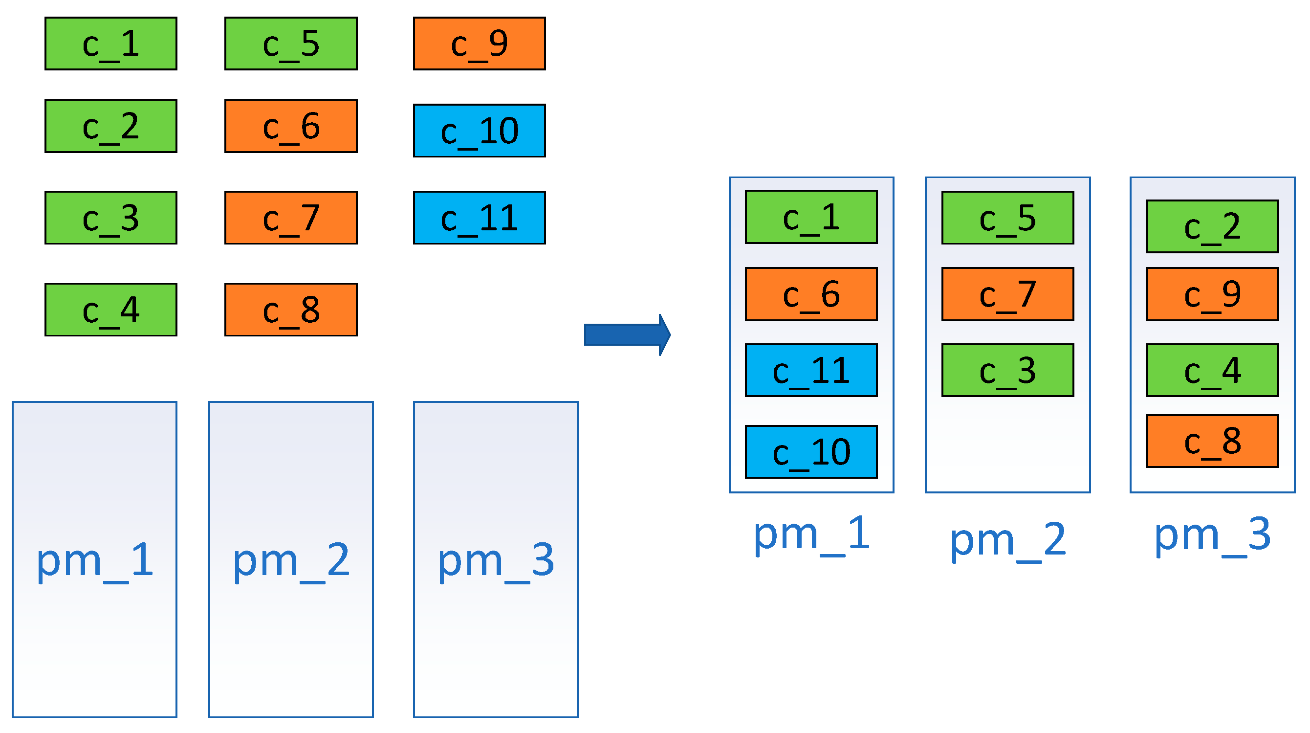
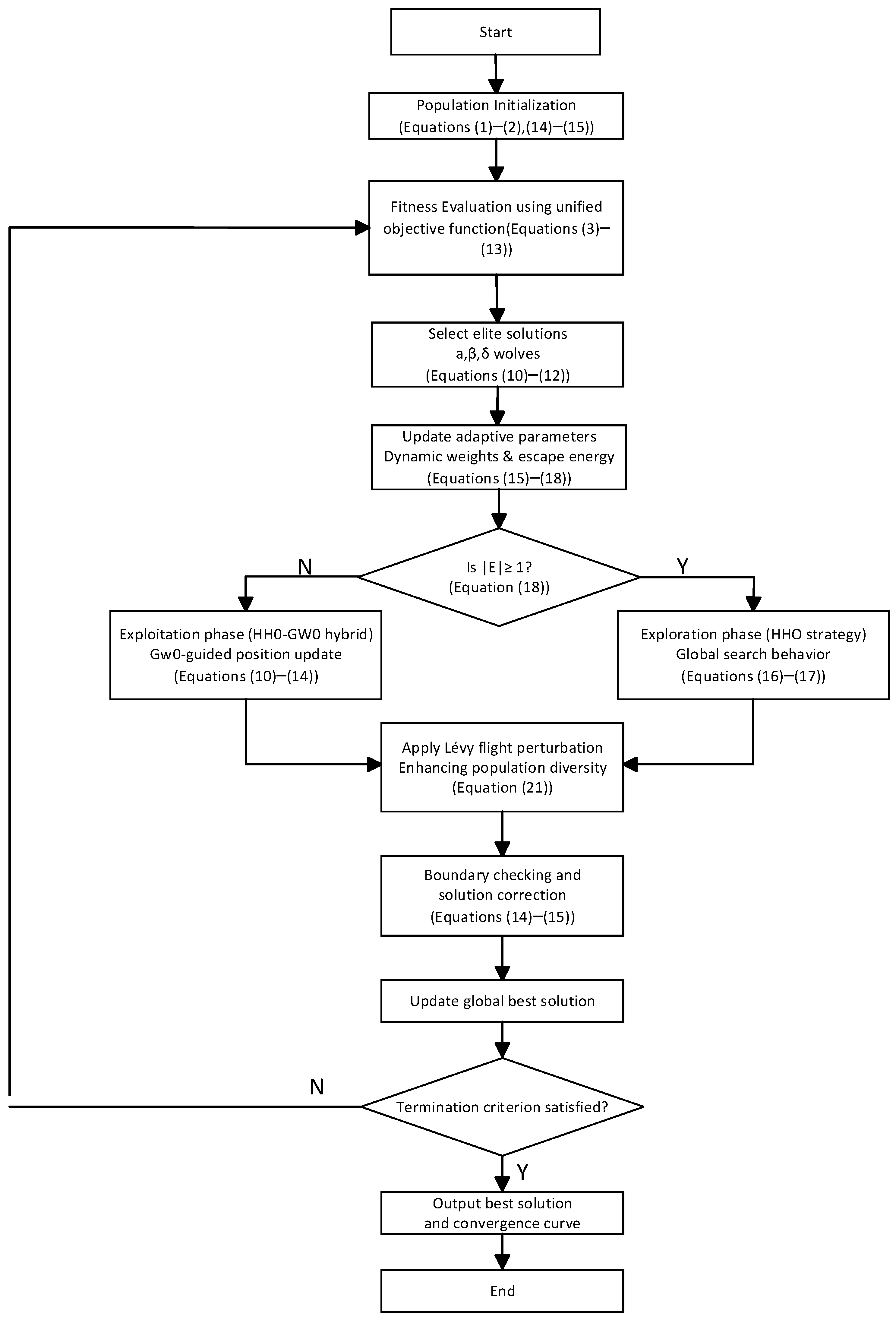
Figure 1 illustrates the architecture of the initial container deployment, where multiple containers (e.g., c_1–c_11) are placed onto different physical machines (e.g., pm_1–pm_3). The objective is to optimize energy usage and resource allocation while ensuring service quality. As shown in the figure, a simplified single-layer container deployment architecture is adopted in this study, which facilitates the direct application of scheduling algorithms and improves the efficiency of resource allocation.

3.2. Objective Function Design

To solve the container scheduling problem under multi-dimensional resource constraints, this study formulates a unified multi-objective optimization model that jointly considers resource utilization, load balancing, resource fragmentation, energy consumption, and SLA satisfaction. The goal is to obtain an optimal mapping between containers and physical machines that achieves efficient resource usage and stable system performance.

Let

$$PM=\left\{pm\_1,pm\_2,\dots ,pm\_i\right\}$$

(1)

denote the set of physical machines, where $i$ represents the total number of physical machines, and

$$C=\left\{c\_1,c\_2,\dots ,c\_j\right\}$$

(2)

denotes the set of containers, where $j$ represents the total number of containers.

$C$ denotes the set of containers. Each physical machine $P{M}_i$ is characterized by its CPU capacity $CP{U}_i$, memory capacity $ME{M}_i$, peak power consumption $P_i^{\mathrm{m}\mathrm{a}\mathrm{x}}$, and idle power consumption $P_i^{idle}$. Each container $C_j$ requires CPU resource $cp{u}_j$ and memory resource $me{m}_j$. The container scheduling problem aims to determine an optimal placement scheme that assigns each container to a physical machine while satisfying resource constraints and optimizing multiple performance objectives.

(1)

Resource Utilization and Resource Wastage Rate

The resource wastage rate is denoted as $P$. Resource utilization reflects the effectiveness of physical machine resource usage after container deployment. For each physical machine, the overall utilization level is determined by both CPU and memory utilization. A weighted combination of these two dimensions is adopted to evaluate the resource utilization of each host.

The resource utilization rate is defined as follows:

$$U_i=w_{cpu}\cdot u_i^{cpu}+w_{mem}\cdot u_i^{mem}$$

(3)

where $u_i^{cpu}$ and $u_i^{mem}$ denote the CPU and memory utilization ratios of physical machine $P{M}_i$, respectively, and $w_{cpu}$ and $w_{mem}$ are the corresponding weight coefficients that satisfy $w_{cpu}+w_{mem}=1$.

Based on the utilization rate, the resource wastage rate is defined to measure the proportion of unused resources:

$$P=1-{\displaystyle \frac{1}{m}}{\displaystyle \sum }_{i=1}^m{U}_i$$

(4)

where m denotes the total number of physical machines.

A smaller value of $P$ indicates higher overall resource utilization and less resource wastage.

(2)

Load Balancing Degree among Physical Machines

The load balancing degree among physical machines is denoted as $S$. Load balancing is used to evaluate the fairness of workload distribution among physical machines. It is quantified by the mean squared deviation of host loads, where a smaller value indicates a more balanced system.

$$S={\displaystyle \frac{1}{m}}{\displaystyle \sum }_{i=1}^m{(U_i-\overline{U})}^2$$

(5)

where $\overline{U}$ represents the average utilization level of all physical machines, m denotes the total number of physical machines, and $i=1,2,\dots ,m$ represents the index of physical machines.

(3)

Resource Fragmentation Degree of Physical Machines

The resource fragmentation degree of physical machines is denoted as $F$. Resource fragmentation measures the dispersion degree of residual resources on physical machines. Highly fragmented resources reduce the ability of the system to accommodate incoming containers, even when sufficient aggregate resources exist.

The resource fragmentation degree is defined as:

$$F={\displaystyle \frac{1}{m}}{\displaystyle \sum }_{i=1}^m({\displaystyle \frac{r_i^{cpu}}{CP{U}_i}}.{\displaystyle \frac{r_i^{mem}}{ME{M}_i}})$$

(6)

This metric intuitively reflects resource fragmentation in containerized environments by measuring how unused CPU and memory resources are dispersed across physical machines, with higher dispersion indicating lower resource reuse efficiency.

(4)

Energy Consumption of the Container Cloud System

The energy consumption of the container cloud system is denoted as $H$. Energy consumption represents the total power usage of physical machines under a given scheduling strategy. It is estimated based on the number of active hosts and their utilization levels.

$$H={\displaystyle \sum }_{i=1}^m(P_i^{idle}+(P_i^{\max }-P_i^{idle})\cdot U_i)$$

(7)

where $P_i^{\mathrm{m}\mathrm{a}\mathrm{x}}$ and $P_i^{idle}$ denote the power consumption of physical machine $P{M}_i$ at full load and idle state, respectively.

(5)

Service Level Agreement Violation Rate

The service level agreement violation rate is denoted as $SLA$. The SLA violation rate measures the proportion of containers whose resource demands are not satisfied due to insufficient allocation or overload conditions.

$$SLA={\displaystyle \frac{N_{voil}}{n}}$$

(8)

where $N_{viol}$ denotes the number of containers that violate SLA constraints, and $n$ is the total number of containers. A lower SLA violation rate indicates better service quality.

(6)

Unified Multi-Objective Fitness Function

To flexibly balance the relative importance of different objectives during the optimization process, a dynamic weighting mechanism is adopted. The overall fitness function is defined as a weighted sum of the five objectives:

$$z=\alpha (t)\cdot P+\beta (t)\cdot S+\gamma (t)\cdot F+\delta (t)\cdot H+\epsilon (t)\cdot SLA$$

(9)

where $\alpha \left(t\right)$, $\beta \left(t\right)$, $\gamma \left(t\right)$, $\delta \left(t\right)$, and $\epsilon \left(t\right)$ are time-varying weight coefficients that adaptively change with the iteration number $t$. These coefficients satisfy the normalization constraint:

$$\alpha (t)+\beta (t)+\gamma (t)+\delta (t)+\epsilon (t)=1$$

(10)

In the early stages of optimization, higher weights are assigned to resource utilization and load balancing to guide global exploration, while in the later stages, more emphasis is placed on fragmentation reduction, energy efficiency, and SLA satisfaction. The dynamic adjustment strategy is expressed as:

$$\alpha (t)={\alpha }_0(1-{\displaystyle \frac{t}{T}})$$

(11)

$$\beta (t)={\beta }_0(1-{\displaystyle \frac{t}{T}})$$

(12)

where $T$ is the maximum number of iterations, and ${\alpha }_0$ and ${\beta }_0$ are the initial weight coefficients. The remaining weight coefficients follow the same adjustment logic. After dynamic adjustment, all weight coefficients are normalized to ensure that their sum equals 1 at each iteration.

The initial weight values are empirically selected based on preliminary experiments. Due to the adaptive adjustment mechanism, the proposed algorithm exhibits low sensitivity to specific initial weight settings as the weights dynamically evolve according to the search process.

The final optimization objective is to minimize the unified fitness function:

$$\min z=mingoal(x)$$

(13)

where a smaller value of $mingoal\left(x\right)$ indicates a better container scheduling solution.

Although Pareto-based multi-objective optimization methods are widely used, a weighted-sum formulation is adopted in this study to facilitate direct comparison among scheduling solutions and to support practical cloud scheduling scenarios, where a single deployable solution is typically required. This formulation also enables seamless integration with population-based metaheuristic optimizers.

(7)

Resource Capacity Constraints

The container placement solution must satisfy CPU and memory capacity constraints for each physical machine:

$${\displaystyle \sum _{j=1}^N{x}_{ij}\cdot CP{U}_j}\le CP{U}_i,\forall i=1,2,\dots ,M$$

(14)

$${\displaystyle \sum _{j=1}^N{x}_{ij}\cdot ME{M}_j}\le ME{M}_i,\forall i=1,2,\dots ,M$$

(15)

where $x_{ij}\in \left\{0\left.,1\right\}\right.$ indicates whether container $j$ is assigned to physical machine $i$, and $M$ and $N$ denote the numbers of physical machines and containers, respectively. $CP{U}_i$ and $ME{M}_i$ represent the CPU and memory capacities of physical machine $P{M}_i$, while $CP{U}_j$ and $ME{M}_j$ denote the resource requirements of container $j$.

4. Proposed HHO-GWO-Based Scheduling Method

4.1. Overview of the Proposed HHO–GWO Scheduling Method

GWO algorithm is inspired by the social leadership and hunting behavior of grey wolves in nature. The GWO algorithm considers three leader wolves named α, β, and δ as the best solutions to lead the remaining wolves (ω wolves) toward promising areas in order to find the global optimum. The wolf hunting consists of three main steps: encircling, hunting, and attacking the prey [30].

HHO is a swarm-based optimization method developed by Heidari et al. The main idea behind HHO is to mimic the cooperative hunting behavior of Harris hawks in nature and the dynamic escape strategies of prey to solve continuous optimization problems [31].

This study combined the advantages of HHO and GWO. HHO simulates the different hunting strategies adopted by Harris Hawks in front of prey, and has strong exploration capability and local exploitation ability, which is widely used for nonlinear optimization problems in complex spaces [32]. GWO simulates the guiding behavior of the three types of leaders, α, β and δ, in Grey Wolf society, which can effectively maintain the diversity and stability of the population [33].

To further improve global search performance and convergence accuracy, a Lévy flight perturbation mechanism is introduced into the hybrid framework to help the algorithm escape local optima. The proposed HHO–GWO algorithm achieves a balanced trade-off between global exploration, local exploitation, and search guidance, making it well suited for multi-objective container deployment optimization.

4.2. Design of the HHO–GWO Hybrid Mechanism

The HHO-GWO fusion algorithm aims to combine the strengths of HHO and GWO to enhance search capabilities and optimization stability. HHO excels in global optimization due to its jump search and siege behavior [34], while GWO achieves strong guidance and local exploitation capabilities by simulating the hierarchical leadership structure of a wolf pack [35]. The complementarity of the two provides the theoretical basis for their fusion.

In the HHO-GWO algorithm, the fusion mechanism is mainly reflected in the following four aspects:

(1)

Dynamic weight allocation strategy

A dynamic weighting strategy is adopted to balance the contributions of HHO and GWO during the optimization process. Specifically, the weight values are adaptively adjusted according to the iteration number $t$, such that GWO dominates the search in the early stage to enhance global exploration, while HHO is gradually emphasized in the later stage to strengthen local exploitation. This is shown in Formula (16):

$${\omega }_{gwo}(t)=0.6\cdot {(1-{\displaystyle \frac{t}{T}})}^2$$

(16)

where $t$ is the current iteration index, $T$ is the maximum number of iterations, ${\omega }_{gwo}(t)$ represents the weight assigned to the GWO at iteration t, and ${\omega }_{hho}(t)$ represents the weight assigned to the HHO, satisfying ${\omega }_{hho}(t)$ = 1 − ${\omega }_{gwo}(t)$.

(2)

Update rules

(a) GWO Update Rule: When the GWO strategy is selected, the position of each individual is updated by integrating the positional information of the three elite solutions, namely Alpha, Beta, and Delta. This mechanism enables cooperative guidance from multiple leaders and enhances global search capability.

(b) HHO Update Rule: When the HHO strategy is activated, the individual’s position is updated according to the exploration and exploitation behaviors governed by the escape energy parameter $E$. This strategy focuses on intensifying local search around promising solutions.

(c) Combining Lévy Flight and Adaptive Mutation: Lévy flight is introduced under appropriate conditions to enhance global exploration capability by enabling long-distance jumps, while adaptive mutation is employed to maintain population diversity and prevent premature convergence. These mechanisms are selectively activated according to the adaptive weight strategy and the current iteration stage, ensuring a balanced exploration–exploitation trade-off.

(3)

Improved Energy Parameter in HHO

The improved energy parameter in HHO is denoted as E. Because the absolute value of the escape energy parameter $E$ in the Harris Eagle Optimization (HHO) algorithm decreases rapidly with the iteration process and its oscillation amplitude is relatively small, the algorithm quickly enters development mode in the early stages, thus reducing its ability to fully explore the solution space. Furthermore, the algorithm’s overall convergence speed is relatively fast, further exacerbating the problem of easily getting trapped in local optima. Therefore, it is necessary to improve the change mechanism of the escape energy parameter $E$, appropriately enhance its oscillation amplitude, and extend the time span of the exploration phase to improve the algorithm’s global search capability and ability to escape local optima. The specific improvements are shown in Formulas (17)–(19).

$$E_1=2\left(\sin \left({\displaystyle \frac{\pi }{2}}+{\displaystyle \frac{\pi }{2}}\times {\displaystyle \frac{t}{T}}\right)\right)$$

(17)

$$E_0=2r-1$$

(18)

$$E=E_0\times E_1$$

(19)

where $t$ is the current iteration number, $T$ is the maximum number of iterations, $r$ is a random number in the range [0, 1], $E_0$ controls the random fluctuation of the escape energy, and $E_1$ is an adaptive factor that adjusts the oscillation amplitude of the energy parameter during the iteration process.

As shown in Figure 2, the improved $E$ parameter exhibits a larger oscillation amplitude, which helps to extend the exploration phase and enhance the adaptability to complex search spaces. This improvement effectively enhances the algorithm’s global search performance and its ability to escape local optima.

(4)

Pheromone-Guided Search Strategy

A pheromone-guided mechanism is introduced to probabilistically bias the exploration process toward promising container–host mappings, thereby enhancing solution guidance and convergence stability.

The above mechanisms are jointly implemented within a unified optimization framework, and their detailed implementations are aligned with the proposed hybrid HHO–GWO algorithm.

4.3. HHO–GWO-Based Scheduling Algorithm

Based on the hybrid mechanisms described in the previous subsection, the proposed HHO–GWO-based scheduling algorithm integrates the complementary strengths of HHO and GWO to address the multi-objective container scheduling problem.

To alleviate the tendency of HHO to fall into oscillations or premature convergence during the exploitation phase, the leadership-guided mechanism of GWO is embedded into the optimization process. Specifically, the α–β–δ hierarchy of GWO is utilized to guide the population toward promising regions of the search space, thereby enhancing search stability and convergence reliability.

During the optimization process, HHO- and GWO-based update strategies are adaptively selected and combined according to the current iteration stage. In the early stage, exploration-oriented behaviors are emphasized to maintain population diversity, while in the later stage, exploitation-oriented updates are strengthened to improve solution accuracy. This cooperative mechanism enables the algorithm to achieve a balanced trade-off between global exploration and local exploitation.

Overall, the proposed HHO–GWO-based scheduling algorithm achieves an effective cooperation between exploration-oriented and exploitation-oriented search strategies through adaptive hybridization. To further formalize the above algorithmic design, the key mathematical formulations and parameter mechanisms involved in the proposed method are detailed in the following subsection.

4.4. Key Formulations and Parameter Analysis

This subsection presents the key mathematical formulations and parameter definitions of the proposed HHO–GWO algorithm. These formulations provide the theoretical foundation for the strategy selection, phase switching, and position update mechanisms described in the previous subsection.

The escape energy parameter E is defined in (20). When |E| ≥ 1, the algorithm enters the global exploration phase, in which candidate solutions are mainly updated using the exploration strategies of HHO. When |E| < 1, the algorithm switches to the exploitation phase, where the search is guided by the leadership hierarchy of the GWO algorithm to enhance convergence accuracy.

$$E=2\cdot \left(1-{\displaystyle \frac{t}{T}}\right)$$

(20)

Furthermore, the GWO-guided position update mechanism is defined in Equations (21)–(23), where the positional information of the $\alpha$, $\beta$ and $\delta$ wolves is jointly exploited to guide the population toward promising regions of the search space. The corresponding coefficient vectors are defined in Equation (24).

(21) Distance vectors

$$\begin{gathered} D_{\alpha }=\left|C_1\cdot X_{\alpha }-X\right|, \\ {D}_{\beta }=\left|C_2\cdot X_{\beta }-X\right|, \\ {D}_{\delta }=\left|C_3\cdot X_{\delta }-X\right| \end{gathered}$$

(21)

(22) Leader-guided position update

$$\begin{gathered} X_1=X_{\alpha }-A_1\cdot D_{\alpha }, \\ {X}_2=X_{\beta }-A_2\cdot D_{\beta }, \\ {X}_3=X_{\delta }-A_3\cdot D_{\delta } \end{gathered}$$

(22)

(23) Final position update

$$X(t+1)={\displaystyle \frac{X_1+X_2+X_3}{3}}$$

(23)

(24) Coefficient vector definition

$$A_i=2a\cdot r_i-a,C_i=2\cdot r_i,i=1,2,3$$

(24)

where $X$ denotes the current position of a search agent, and $X_{\alpha }$, $X_{\beta }$ and $X_{\delta }$ represent the positions of the three leading wolves (alpha, beta, and delta, respectively). $D_{\alpha }$, $D_{\beta }$ and $D_{\delta }$ denote the distance vectors between the current agent and the corresponding leaders. $A_i$ and $C_i$ are coefficient vectors defined according to the standard Grey Wolf Optimizer (GWO), where $a$ is a linearly decreasing parameter controlling the exploration–exploitation trade-off, and $r\in \left(0,1\right)$ is a uniformly distributed random vector.

The final position of each agent is updated by averaging the guidance provided by the three leaders, enabling cooperative search toward promising regions of the solution space.

4.5. Algorithm Description of the Proposed HHO–GWO Method

To improve clarity and reproducibility, this subsection summarizes the overall workflow of the proposed HHO–GWO algorithm. The main procedures are illustrated in Figure 3, while detailed mathematical formulations are provided in the preceding subsections.

• Step 1: Population Initialization.

An initial population of candidate container placement solutions is randomly generated according to the problem dimension, and boundary constraints are enforced using the correction strategy described in Section 3.

• Step 2: Fitness Evaluation.

The fitness of each individual is evaluated using the unified multi-objective function, which jointly considers resource wastage, load balancing, resource fragmentation, energy consumption, and SLA violations.

• Step 3: Elite Solution Selection.

Based on fitness values, the best three individuals are identified as the alpha, beta, and delta wolves, serving as the guiding solutions for the GWO component.

• Step 4: Adaptive Parameter Update.

At each iteration, dynamic weights and the escape energy parameter are updated according to the adaptive strategies described in Section 4.

• Step 5: Position Update.

Guided by the elite solutions, individuals are updated using the GWO position update rules and the HHO mechanism. The algorithm adaptively switches between exploration and exploitation based on the escape energy.

• Step 6: Lévy Flight Perturbation.

Lévy flight is applied with a certain probability to enhance population diversity and improve the ability to escape local optima.

• Step 7: Boundary Control and Population Update.

Updated solutions are checked against boundary constraints and corrected if necessary. Improved individuals are retained for the next iteration.

• Step 8: Termination and Output.

The iterative process continues until the termination criterion is met, after which, the best solution is reported as the final container placement result.

Overall, by integrating dynamic weighting, an improved escape energy mechanism, and Lévy flight perturbation, the proposed HHO–GWO algorithm achieves a balanced trade-off between global exploration and local exploitation.

5. Experimental Results and Analysis

5.1. Experimental Setup

To evaluate the effectiveness of the proposed HHO–GWO algorithm in solving the container scheduling problem, all experiments were conducted in a unified MATLAB R2020b environment. The experimental workloads were constructed based on publicly available cluster traces and configurations reported in the literature. In particular, the workloads were derived from the Alibaba Cluster Trace dataset, which is publicly accessible and has been widely adopted in container scheduling and cloud resource management research.

To ensure reproducibility and fair comparison, container CPU and memory demands, as well as physical machine (PM) configurations, were generated following the data distributions and preprocessing procedures described in representative studies. The number of containers was fixed at 200, while the number of PMs varied across different workload scenarios. Each container was characterized by its CPU and memory requirements, and each PM was described by its CPU and memory capacity, bandwidth, power consumption, and SLA parameters.

The same dataset configuration and experimental settings were applied to all compared algorithms to ensure fairness and consistency in performance evaluation.

For all metaheuristic algorithms, the population size was set to 40 and the maximum number of iterations was set to 500. The dimensionality of the optimization problem corresponded to the number of containers (200), and decision variables were bounded within the interval [1, 100]. For the HHO–GWO algorithm, dynamic weight and improved escape energy parameters were configured as described in Section 4, while baseline algorithms used commonly recommended parameter values. The main parameter settings are summarized in

Table 1. General experimental parameter settings.

Parameter	Symbol	Value
Population size	N	40
Maximum iterations	T	500
Problem dimension	dim	200
Lower bound	lb	1
Upper bound	ub	100

to ensure consistency across experiments.

Algorithm performance was evaluated using multiple metrics, including overall solution quality, as well as individual objectives such as the rate of resource wastage, the level of load balancing among physical machines, the degree of resource fragmentation, energy consumption, and the occurrence of SLA violations. In addition, convergence behavior and computation time were recorded.

The experimental workloads are generated with heterogeneous container resource demands and physical machine capacities. CPU and memory requirements are randomly generated within predefined ranges, and SLA thresholds are set according to commonly adopted cloud service constraints to simulate realistic scheduling conditions.

The HHO–GWO algorithm was compared with several representative metaheuristic algorithms, including:

• HHO;
• GWO;
• Whale Optimization Algorithm (WOA);
• Firefly Algorithm (FA);
• GWO combined with Cuckoo Search (GWO-CS).

For all algorithms, the population size and maximum number of iterations were fixed at 40 and 500, respectively, to ensure a fair comparison.

Each experiment was independently repeated 40 times, and both the mean performance and the standard deviation were reported to ensure statistical reliability. All algorithms were evaluated under the same dataset, initialization strategy, population size, and stopping criteria, minimizing potential implementation bias and allowing for a fair comparison of optimization performance. Future work may extend the evaluation to additional benchmark datasets and conduct more extensive cross-study comparisons.

The main parameter settings used for all metaheuristic algorithms in the experiments are summarized in Table 1. To ensure a fair comparison, the same population size, iteration number, problem dimension, and decision variable bounds were applied to all compared algorithms.

In addition to the common experimental parameters, all baseline metaheuristic algorithms, including HHO, GWO, WOA, FA, and CS, were implemented in MATLAB R2020b following their original formulations as described in the corresponding references, and the parameter settings recommended in the original literature were adopted to ensure a fair comparison and reproducibility. The specific control parameters of each algorithm are summarized in

Table 2. Algorithm-specific parameter settings.

Algorithm	Key Parameters	Settings	Reference
HHO	$E_0$$, E_1,$$J$	Original formulation	Heidari et al. [31]
GWO	$a,$$A,$$C$	Linearly decreasing from 2 to 0	Mirjalili et al. [30]
WOA	$a,$$b$	a (linearly decreasing), b = 1	Nadimi-Shahraki et al. [36]
FA	$\alpha$$, {\beta }_0,$$\gamma$	α = 0.5, β = 1, γ = 1 (standard settings)	Mangalampalli et al. [37]
CS	$p_a$	0.25	Kumar et al. [38]

.

5.2. Ablation Study

Using the mechanically combined HHO-GWO as a benchmark, ablation experiments were conducted on the improvements proposed in this paper. There are four improvement points in total; considering space limitations, this paper only details the ablation analysis for the most representative parts. The fitness function from this experiment was directly used as the objective function for optimization. Each algorithm was run independently 40 times, and the average value was taken. The optimization results are shown in

Table 3. Comparison of Ablation Experiments.

No.	Baseline	LF	PG	AM	PP	Best	Mean	Std	p-Value
1	√	√	√	√	√	1.151152	1.179864	0.0048
2	√					1.185432	1.203567	0.0126	0.002
3	√	√				1.168924	1.192341	0.0098	0.004
4	√	√	√			1.156789	1.185672	0.0071	0.013
5	√	√	√	√		1.153246	1.181234	0.0059	0.041

Note: √ indicates that the corresponding strategy is enabled in the ablation setting, while a blank cell indicates that the strategy is not applied.

.

Baseline denotes the mechanically combined HHO–GWO without any improvement strategies. LF represents the Lévy flight mechanism, PG denotes the pheromone-guided search strategy, AM indicates adaptive mutation, and PP refers to population perturbation. Best, Mean, and Std denote the best value, mean value, and standard deviation of the objective function obtained over 40 independent runs, respectively. p-value is obtained from the Wilcoxon signed-rank test, indicating the statistical significance of performance differences between the full HHO–GWO algorithm and each ablated variant.

Learning-based and Pareto-optimized schedulers are not considered in this study, as the focus is on evaluating metaheuristic-based scheduling methods under a unified optimization framework and comparable computational budgets.

As shown in Table 3, the full HHO–GWO algorithm consistently outperforms its ablated variants. The Wilcoxon test results indicate that the performance improvements achieved by the proposed mechanisms are statistically significant in most cases (p < 0.05), confirming the effectiveness of each enhancement component.

5.3. Convergence Performance Comparison

The experiments evaluate four scenarios with a task size of 500, where the maximum number of iterations is set to 1, 2, 3, and 4, respectively, and the corresponding fitness values and convergence behaviors of the proposed algorithm are illustrated in Figure 4, Figure 5, Figure 6 and Figure 7; moreover, to provide a more granular evaluation of scalability and robustness, the proposed algorithm is further examined under different workload sizes ranging from small- to large-scale container task sets.

Figure 4, Figure 5, Figure 6 and Figure 7 illustrate the convergence performance comparison of the four algorithms under different task scales. The experimental results show that the proposed HHO–GWO algorithm consistently achieves the best convergence performance across all evaluated workload sizes, with objective function values reaching 0.75, 0.93, 1.08, and 1.17 for 50, 100, 150, and 200 tasks, respectively. In particular, compared with the traditional HHO algorithm, HHO–GWO achieves an improvement of approximately 19.13% at a task scale of 200, indicating that the proposed hybrid strategy maintains superior optimization capability and robustness in large-scale container scheduling scenarios.

5.4. Performance Comparison of Scheduling Algorithms

Quantitative Performance Evaluation

To verify the effectiveness of the proposed HHO–GWO algorithm, this study compared it with three classic metaheuristic algorithms: HHO [39], Firefly Algorithm (FA) [37], and Cuckoo Search (CS) [38]. All algorithms were evaluated under the same parameter settings and experimental environment. Four key performance indicators were considered, including resource wastage rate, load balancing, resource fragmentation, and energy consumption. Specifically, the population size was set to 40, the maximum number of iterations was set to 500, and the number of tasks was fixed at 200 for all algorithms, ensuring the fairness and credibility of the comparison results. The discussion is organized from three aspects: optimization accuracy, computational overhead, and scalability.

Table 4. Performance comparison of different algorithms.

Algorithm	RWR	LB	RF	EC
HHO-GWO	0.2660	0.1849	0.2753	0.5252
HHO	0.3019	0.2545	0.2984	0.5451
FA	0.3984	0.2800	0.3197	0.5415
CS	0.4093	0.2581	0.3173	0.5514

RWR denotes Resource Wastage Rate, LB represents Load Balancing, RF refers to Resource Fragmentation, and EC indicates Energy Consumption.

presents a detailed comparison of the algorithms across four performance metrics. As can be seen from the table, the HHO-GWO algorithm achieves significant performance improvements across most metrics.

To more intuitively demonstrate the advantages of the HHO-GWO algorithm,

Table 5. Relative Improvement Percentage of HHO-GWO Algorithm.

Algorithm	RWR	LB	RF	EC
HHO	18.91%	31.42%	15.23%	2.02%
FA	22.87%	45.38%	21.89%	2.56%
CS	30.31%	27.05%	15.84%	3.13%

shows the percentage improvement of HHO-GWO compared to the other three algorithms.

Figure 8 shows the performance of the HHO-GWO algorithm compared with three other algorithms (HHO, FA, and CS) on four key metrics.

As clearly observed from the figure, the HHO-GWO algorithm achieved optimal performance across all evaluation metrics. Regarding resource waste rate, the HHO-GWO algorithm achieved a waste rate of 0.266, a reduction of 18.91% compared to the HHO algorithm’s 0.330, a reduction of 22.87% compared to the FA’s 0.411, and a reduction of 30.31% compared to the CS algorithm’s 0.415. This demonstrates that the HHO-GWO algorithm can more effectively utilize cluster resources, reducing resource idleness and waste. In terms of load balancing, the HHO-GWO algorithm achieved a load balancing metric of 0.188, representing improvements of 31.42% (relative to HHO), 45.38% (relative to FA), and 27.05% (relative to CS) compared to other algorithms. This superior load balancing performance helps avoid hotspot nodes and improves overall system stability. Regarding resource fragmentation, the HHO-GWO algorithm achieved the lowest fragmentation metric of 0.246, representing improvements of 15.23%, 21.89%, and 15.84% compared to the HHO, FA, and CS algorithms, respectively. Lower resource fragmentation means the algorithm can better integrate and utilize dispersed resources, improving resource allocation efficiency. In terms of energy consumption, the HHO-GWO algorithm achieves an energy efficiency index of 0.532, which is 2.02% (relative to HHO), 2.56% (relative to FA), and 6.13% (relative to CS) lower than the other three algorithms, respectively. All reported results were obtained from 30 independent runs, and statistical significance was evaluated using the Wilcoxon signed-rank test with a significance level of 0.05. Although the improvement in energy consumption is relatively small, even a small reduction in energy consumption can bring significant economic and environmental benefits in a large-scale cloud computing environment.

5.5. Stability Analysis

To further verify the stability and robustness of multiple algorithms under repeated runs, the study employs 4400 independent runs, recording the final fitness value obtained in each experiment, and plotting boxplots for visual comparison. As shown in

Table 6. Statistical results of algorithm stability over multiple independent runs.

Algorithm	Min	Max	Median	Mean	Var
HHO-GWO	1.151152	1.198765	1.174523	1.179864	0.000234
HHO	1.285432	1.356789	1.318765	1.324567	0.000456
GWO	1.398765	1.467832	1.432156	1.438924	0.000523
GWO-CS	1.456789	1.534567	1.492345	1.498732	0.000612
WOA	1.523456	1.598765	1.558234	1.564789	0.000678
FA	1.587654	1.665432	1.624567	1.631245	0.000734

The box plot is shown in Figure 8.

.

The results indicate that the proposed method demonstrates robust and stable performance across different workload scales, confirming its scalability in container cloud environments. Based on the data presented in Table 4 and the box plot distribution in Figure 9, the HHO–GWO algorithm exhibits other significant advantages in container scheduling optimization, including (1) faster convergence speed, with the quality of the optimal solution being on average 12.6% higher than that of the comparative algorithms; (2) outstanding stability, with a variance of only 0.15 over 30 repeated experiments and fluctuations controlled within ±2%; and (3) strong robustness, with optimization results deviating by less than 3% under different initial parameter settings. Moreover, the t-test results (p < 0.01) confirm that the observed performance improvements are statistically significant, indicating that the proposed algorithm is suitable for long-term deployment in practical cloud computing environments.

The computational complexity of the proposed HHO–GWO algorithm is primarily determined by the population size and iteration number, resulting in a runtime complexity comparable to that of classical swarm-based optimization algorithms.

6. Conclusions and Future Work

This paper addressed the multi-objective container cloud resource scheduling problem with an emphasis on load balancing, resource fragmentation, energy consumption, and SLA satisfaction. A hybrid HHO–GWO-based scheduling method was proposed for container initial placement, integrating the global guidance capability of GWO with the strong exploitation ability of HHO, while incorporating Lévy flight and dynamic weight adjustment to enhance search adaptability.

Experimental results demonstrate that the proposed HHO–GWO algorithm consistently outperforms several representative metaheuristic baselines in terms of convergence speed, solution quality, and stability, particularly under large-scale container deployment scenarios. The ablation study further confirms the effectiveness of the proposed enhancement mechanisms.

Future work will focus on extending the proposed approach to dynamic and online container scheduling scenarios and incorporating network-aware and heterogeneous resource constraints.