Abstract
As smart cities evolve, the demand for real-time, secure, and adaptive network monitoring, continues to grow. Software-Defined Networking (SDN) offers a centralized approach to managing network flows; However, anomaly detection within SDN environments remains a significant challenge, particularly at the intelligent edge. This paper presents a conceptual Kafka-enabled ML framework for scalable, real-time analytics in SDN environments, supported by offline evaluation and a prototype streaming demonstration. A range of supervised ML models covering traditional methods and ensemble approaches (Random Forest, Linear Regression & XGBoost) were trained and validated using the InSDN intrusion detection dataset. These models were tested against multiple cyber threats, including botnets, dos, ddos, network reconnaissance, brute force, and web attacks, achieving up to 99% accuracy for ensemble classifiers under offline conditions. A Dockerized prototype demonstrates Kafka’s role in offline data ingestion, processing, and visualization through PostgreSQL and Grafana. While full ML pipeline integration into Kafka remains part of future work, the proposed architecture establishes a foundation for secure and intelligent Software-Defined Vehicular Networking (SDVN) infrastructure in smart cities.
1. Introduction
Intelligent edge environments (IEEs) represent a distributed computing paradigm that brings data processing and analysis closer to the source of data generation, the edge of the network. Rather than relying solely on centralized cloud infrastructure, IEEs leverage local compute, storage, and networking resources to perform tasks in real-time or near real-time. This proximity enables faster response times, reduced latency, improved bandwidth utilization, and enhanced privacy and security. Emerging technologies such as Multi-access Edge Computing (MEC), the Internet of Things (IoT), and Machine Learning (ML) have strengthened IEEs, enabling sustainable and high-quality services in smart cities [1]. Smart cities depend heavily on data to optimize urban operations, improve citizen services, and enhance quality of life. IEEs provide the infrastructure to collect, process, and analyze this data in a timely and efficient manner. The relationship between IEEs and smart cities is mutually reinforcing: IEEs support the functionality of smart city applications, while smart cities provide the context and use cases for deploying IEEs. For example, in Smart Transportation [2], IEEs can monitor traffic flow, optimize traffic signals, and deliver real-time information to drivers. Data from traffic cameras and sensors can be processed at the edge to detect congestion, accidents, and other incidents, enabling faster responses and improved traffic management. In Smart Healthcare [3], IEEs facilitate remote monitoring and healthcare delivery. Wearable sensors can collect patient vital signs, which are analyzed at the edge to detect anomalies and provide timely interventions. Similarly, in Smart Energy [4], IEEs enable monitoring of energy consumption, optimization of distribution, and integration of renewable energy sources. Data from smart meters can be processed to identify opportunities for conservation and efficiency. As the complexity of smart city infrastructures grows, the demand for real-time, scalable, and intelligent data management becomes critical. IEEs address this need through a layered architecture that distributes processing, communication, and analytics across edge nodes. The proposed IEE framework consists of seven architectural layers [5], as illustrated in Figure 1.
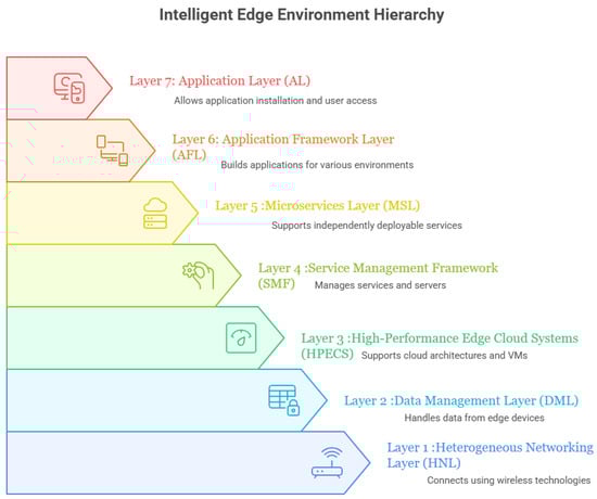
Figure 1.
Layers of an Intelligent Edge Environment.
In parallel, the evolution of Software-Defined Networking (SDN) and Network Function Virtualization (NFV) has transformed modern communication networks by introducing flexibility, programmability, and scalability capabilities vital for dynamic traffic management and improving Quality of Experience (QoE) [6]. However, as SDN/NFV architectures grow more complex, particularly when deployed across IEEs in smart cities, they face significant challenges related to security and real-time anomaly detection. A critical issue in SDN networks is the timely identification and mitigation of anomalies such as distributed denial-of-service (ddos) attacks, botnets, reconnaissance, brute force attempts, and web-based threats [7]. Traditional security mechanisms often lack the adaptability and responsiveness needed to protect dynamic, distributed edge networks effectively. To address these challenges, ML techniques have emerged as promising solutions for anomaly detection within SDN frameworks [8,9]. When combined with real-time data streaming platforms such as Apache Kafka [10], ML models can continuously monitor network traffic and enable fast, automated anomaly detection [11,12]. Trained on SDN-specific intrusion datasets, these models can classify and predict malicious activities, allowing network operators to react promptly and minimize potential damage. This paper proposes a Kafka-enabled SDN framework that integrates real-time streaming with ML-based anomaly detection. While ML models are developed and evaluated offline, the framework incorporates Apache Kafka, PostgreSQL, and Grafana into a Dockerized prototype, simulating a future-ready architecture capable of scalable, low-latency analytics. This approach supports intelligent, adaptive network monitoring and lays the foundation for secure SDVN infrastructure in smart cities. The key contributions of this research are as follows:
- (1)
- A new conceptual framework for SDN attack detection.
- (2)
- Development of secure and intelligent SDN–ML models to support smart city applications.
- (3)
- A Kafka-based prototype for offline data ingestion and processing, including integration of flow metrics into PostgreSQL and visualization dashboards.
- (4)
- Future directions for integrating ML models into SDN controllers for vehicular applications, enabling anomaly classification in edge computing.
The experimental evaluation demonstrates that the proposed framework achieves high accuracy and responsiveness, validating its potential to enhance security and operational intelligence in IEEs. The remainder of this paper is organized as follows: Section 2 reviews related work. Section 3 presents the proposed methodology. Section 4 analyzes the SDN dataset. Section 5 discusses the integration of Apache Kafka with offline dataset streaming and describes the prototype implementation in a VANET testbed for IEEs. Finally, Section 6 concludes the paper.
2. Related Work
Research on anomaly detection in SDN environments has advanced significantly over the past five years. Existing work can be grouped into traditional methods, ML-based techniques, and streaming analytics systems, highlighting the limitations of static models and the promise of real-time, edge-aware solutions.
2.1. Traditional vs. Machine Learning-Based Detection in SDN
Traditional detection in SDN has relied on signature-based or static rule-based systems, which struggle with novel attacks and often suffer from high false positive rates. In contrast, ML methods can adaptively learn patterns from data, enhancing their ability to detect previously unseen threats and reduce false positives. For example, authors in [13] benchmarked classical ML classifiers including Decision Trees (DT), Support Vector Machines (SVM), and Random Forest (RF), using the NSL-KDD dataset. Their results revealed limitations in both accuracy and scalability when applied to SDN environments.
In addition to this, recent research has demonstrated that ML techniques outperform static systems. In [14], deep learning models were applied to SDN anomaly detection, achieving over 99% accuracy with unsupervised neural networks. Similar research [15] demonstrated the effectiveness of Deep Learning (DL) techniques for securing IoT systems via SDN. A more targeted study [16] compared supervised models such as RF, DT, SVM, and XGB on CICddos2019 data, finding that RF was most effective for ddos detection in SDN. Entropy-based methods have also been explored. Studies using Shannon and Renyi entropy [17,18] applied to flow features (e.g., source/destination IP, ports, and flow counts) demonstrated effectiveness against high-volume ddos floods in OpenFlow networks. However, such approaches require careful tuning of windows and thresholds, and they struggle with low-rate, evasive, or multi-modal attacks [19].
2.2. Streaming Analytics and SDN: Kafka and Beyond
Recent studies highlight Apache Kafka as a leading solution for real-time, scalable, and low-latency data streaming [20]. Comparative analyses show Kafka’s advantages in throughput, performance, and integration within modern data warehousing and analytics stacks [21]. Kafka has been widely adopted in event-driven architectures and big data pipelines, where optimized partitioning, broker configuration, and Kafka Connect improve scalability, fault tolerance, and consumer-lag reduction [22]. While Kafka and visualization tools such as Grafana are widely used in domains like IoT and log processing, their adoption for SDN anomaly detection remains limited. This gap highlights the potential of integrating Kafka-driven streaming with ML models for intelligent, real-time monitoring in SDN environments.
Edge-Based ML for Anomaly Detection in SDN
Mobile Edge Computing (MEC) was introduced to reduce cloud overload by enabling computation offloading at the network edge. Recent work [23] explores the integration of SDN and NFV with MEC to enhance flexibility, centralized control, and resource orchestration. Similarly, ref. [24,25] highlight the use of DL for securing networks against cyberattacks and implementing intrusion detection systems in SDNs. Edge-based ML has gained attention for its ability to provide low-latency, context-aware anomaly detection. However, most studies lack full implementation in distributed SDN infrastructures and rarely address real-time updating of ML models at the edge, leaving this as an open challenge.
2.3. Vehicular Networks
The past decade has seen rapid advances in software-defined vehicular networks, driven by the emergence of Connected and Autonomous Vehicles (CAVs) [26,27]. Numerous testbeds [28,29] have supported intensive studies on Intelligent Transportation Systems (ITSs), aiming to reduce travel times, alleviate congestion, and minimize accidents. However, Vehicular networks pose strict requirements: ultra-reliable, low-latency, and high-bandwidth communication combined with real-time processing. Meeting these demands requires a shift from centralized cloud processing to edge-based analysis and computing infrastructures, enabling faster responses and context-aware services at the network’s edge.
2.4. Research Gap
Table 1 summarizes the strengths and limitations of current approaches. Traditional methods are simple to deploy but are static and inflexible. ML-based methods provide higher accuracy and adaptability but often operate in an offline mode. Streaming frameworks such as Kafka offer scalability and low latency but lack direct integration with SDN-specific ML pipelines. Edge-based ML shows promise for fast, localized decision-making but is rarely applied in SDN/NFV contexts.

Table 1.
Summary of Strengths and Gaps in Data Processing Approaches.
3. Proposed Methodology
This section introduces the proposed Kafka-driven SDN framework, its integration with the intelligent edge environment (IEE), the ML based anomaly detection workflow, and the experimental setup. A key challenge in SDN-based networks is the vulnerability of the controller to ddos attacks. When OpenFlow switches receive packets without matching flow rules, they are forwarded to the controller as packet-in messages. Attackers can exploit this behavior by sending large volumes of packets with randomly generated destination addresses. Unlike traditional networks, the attacker does not need to spoof the source address. The resulting surge of packet-in messages can overwhelm the SDN controller, eventually leading to service disruption [30].
3.1. Layered Architecture for Data Management in IEE
The proposed framework focuses on Layer 2: the Data Management Layer (DML) of the IEE, responsible for handling the vast and heterogeneous data generated at the edge (autonomous vehicles, RSUs, and IoT sensors). Figure 2 illustrates the SDN controller integrated within the IEE and details the streaming and detection workflows.
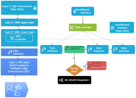
Figure 2.
SDN controller in an Intelligent Edge Environment.
- Layer 1: Heterogeneous Networking Layer (HNL): Collects real-time traffic flows from VANET testbeds and IoT devices. The data is forwarded through SDN-enabled switches.
- Layer 2: Data Management Layer (DML): Divided into upper and lower sublayers. The lower layer incorporates the SDN controller for centralized flow management, which is connected to switches via the Southbound Interface (OpenFlow). The upper layer manages the data pipelines using Apache Kafka for scalable streaming.
- Layer 3: High-Performance Edge Cloud Systems (HPECS]: Provides large-scale processing and storage hosted on cloud platforms (e.g., Azure). The Northbound Interface links the SDN controller with ML analytics modules and orchestration services.
3.2. Kafka-Driven Streaming and Anomaly Detection
The anomaly detection workflow is as follows:
- Traffic flows from the VANET testbed (Layer 1) are ingested into Kafka brokers deployed at the edge (RSUs/MEC servers).
- Data switches forward packets to Kafka topics. Consumers, including ML pipelines, subscribe to real-time inspections.
- The ML model integration module classifies packets into the following:
- -
- Benign traffic: forwarded to the next switch.
- -
- Anomalous traffic → flagged and redirected to the controller for mitigation (e.g., dropping the packet or updating flow rules).
This design ensures scalable ingestion, adaptive traffic routing, and low-latency security enforcement.
3.3. ML Workflow
To enable anomaly detection, we develop supervised ML models trained on SDN-specific datasets (e.g., InSDN). Figure 3 illustrates the ML pipeline and streaming integration:
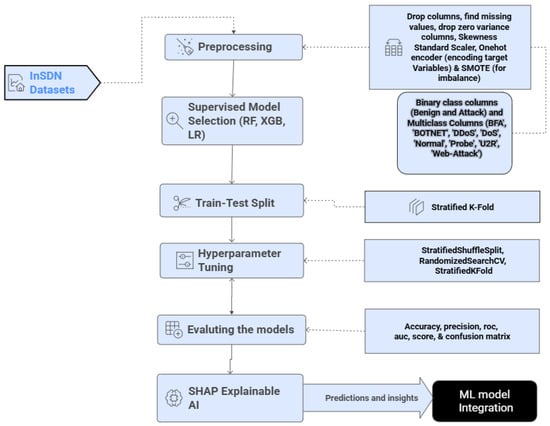
Figure 3.
ML process for SDN Model development.
- Trained models are deployed in the Kafka-SDN framework for real-time inference.
- Predictions drive packet-handling decisions (forward or drop).
3.4. VANET Testbed and MEC Integration
The VANET framework provides a storage platform for mobile users as they move around. Mobile services are migrating to the edge of cloud environments through Mobile Edge Computing (MEC). The objective of this study is to implement a ML model for streaming analysis in SDN controllers and storage within vehicular environments. For instance, if a vehicle on a smart highway suddenly exhibits abnormal traffic patterns, Kafka can be used for data streaming. Vehicles publish sensor and flow data to Kafka topics, and consumers. Kafka brokers at the edge (e.g., RSUs and MEC servers) will function as real-time data collectors.
4. Machine Learning Model Development
The dataset used in this study provides flow-level network telemetry, which is crucial for real-time anomaly detection in SDN environments. It includes attributes such as source and destination IP addresses, port numbers, flow durations, packet/byte counts, protocol types, and class labels that span multiple attack categories. These flow-based features are representative of traffic in intelligent edge environments (IEEs), where heterogeneous devices, such as connected vehicles, IoT sensors, and roadside units, generate diverse but structured traffic patterns.
4.1. Dataset Description
Experiments were conducted on the InSDN dataset [31], which contains 343,889 traffic records with 84 flow-level features. InSDN is an open-source intrusion detection dataset specifically designed for SDN anomaly detection. Each flow is labeled as either benign or one of several attack types (e.g., ddos, dos, probe, botnet, web attack, and U2R). The dataset was distributed across three files:
- Normal_data.csv: Benign traffic, including FTP, DNS, HTTPS, and other services (68,424 records).
- OVS.csv: Attack traffic from an Open vSwitch (OVS) testbed, covering dos, ddos, Port scanning, brute force, web attack, and botnet attacks (138,722 records).
- Metasploitable-2.csv: Attack traffic generated on the Metasploitable-2 VM, including dos, ddos, port scanning, brute force, and U2R (136,743 records).
The merged dataset thus consisted of 343,889 flow records, including 68,424 normal flows and 275,465 attack flows across multiple categories. These include ddos, port scanning (probe), brute force attempts (BFA), web exploitation, botnet command-and-control activity, and privilege escalation attempts (U2R). Therefore, the dataset reflects a wide range of threats targeting SDN controllers and switches. Table 2 summarizes the composition.
Table 2.
InSDN dataset composition.
4.2. Step 1: Dataset Loading and Attack Distribution
All three datasets were merged into a unified structure with a source label for the provenance. Table 3 shows the attack type distribution: ddos (121,942 flows), probe (98,129), dos (53,616), and brute force (1,405) dominate the dataset. Minority classes, such as web (192), botnet (164), and U2R (17), remain critically underrepresented.
Table 3.
SDN-specific attack categories and severity levels.
4.3. Step 2: Data Preprocessing
Prior to training, the merged dataset was subjected to a series of preprocessing steps to ensure data consistency and model readiness. The main preprocessing tasks included handling categorical variables, feature scaling, and addressing class imbalance.
4.3.1. Handling Missing Values and Encoding
The dataset was inspected for missing values, and no NaNs or incomplete entries were detected. Numeric Columns (79): There were columns such as “Flow ID,” “Src IP,” “Dst IP,” and “Timestamp” that were dropped, leaving 79 remaining columns. Summary statistics for these numeric features (mean, standard deviation, minimum, quartiles, maximum) indicated that the data were heavily imbalanced and contained extreme outliers, which could negatively affect ML performance. Additionally, zero-variance columns (12 total), including “Fwd PSH Flags,” “Fwd URG Flags,” “CWE Flag Count,” and “ECE Flag Count,” were identified. Since all rows for these columns had the same value, they provided no useful information for ML and were therefore dropped. Highly skewed columns, such as “Tot Fwd Pkts” (skew = 585) and “TotLen Fwd Pkts” (skew = 326), demonstrated extreme skewness, as forward packets had large values. The total length of forward packets was reduced using log scaling to handle this skewness effectively, which is common in ddos/dos datasets where a small number of attack flows dominate packet counts.
4.3.2. Feature Importance via Mutual Information and Scaling
All numerical features were standardized to ensure that models sensitive to feature magnitudes (e.g., LR) converged efficiently. To assess the relative contribution of each feature towards distinguishing attack classes from benign traffic, Mutual Information (MI) analysis was applied. MI measures the reduction in the uncertainty of the target variable when a given feature is observed, capturing both linear and nonlinear dependencies. Table 4 indicates that features such as Bwd Header Len (MI = 1.247), Dst Port (MI = 1.126), and backward inter-arrival time statistics (Bwd IAT Tot, Bwd IAT Max, Bwd IAT Mean) are among the most informative. Flow-based attributes such as Flow Duration, Flow Pkts/s, and Bwd Pkts/s also ranked highly, reflecting the temporal burstiness of attacks. These results confirm that timing and packet-level statistics are strong indicators of abnormal behaviour in SDN environments. All features were normalized using StandardScaler to achieve zero mean and unit variance while preserving their relative distribution. This scaling ensures that features with different ranges (e.g., ports, durations, bytes/s) are comparable.
Table 4.
Top features ranked by Mutual Information.
4.4. Multi-Class and Binary Label Distribution
Two classification tasks were Performed:
- Multi-class Classification: The original labels were preserved to classify flows into specific attack categories. The label distribution is highly imbalanced, as shown in Table 5, with the majority belonging to probe (98,129 flows) and ddos (73,529 + 48,413 flows), Whereas minority classes, such as U2R, have only 17 instances.
Table 5. Multi-class label distribution in the InSDN Dataset.
- Binary Classification: A second formulation grouped all attack classes as ‘Attack’ and retained ‘Normal’ as benign traffic. This resulted in 275,465 attack flows (80%) and 68,423 benign flows (20%), highlighting a skewed distribution but simplifying the detection task to anomaly versus normal traffic.
The feature space for both tasks consisted of 343,888 flow records and 67 attributes, covering flow durations, packet and byte counts, protocol types, and statistical measures such as inter-arrival times. Among these, the protocol was the only categorical feature and was one-hot encoded, whereas all remaining features were standardized. This preprocessing ensured that the dataset was normalized, consistent, and ready for supervised learning experiments.
4.5. Class Imbalance Handling with SMOTE
The InSDN dataset exhibits a highly imbalanced class distribution, which can bias ML models towards the majority attack types. For example, in the binary task (normal vs. attack), benign traffic represents only 19.9% of the training samples, whereas attack traffic dominates with 80.1%. Similarly, in the multi-class task, categories such as ddos (35.46%) and probe (28.54%) overshadowed rare attacks such as U2R with only 14 samples (0.01%) and botnet with 131 samples (0.05%).
To mitigate this issue, the Synthetic Minority Oversampling Technique (SMOTE) was applied during training to balance the class distribution. SMOTE generates synthetic samples of minority classes in the feature space, thereby preventing over fitting to dominant classes and improving generalization. Table 6 and Table 7 illustrate the class distributions before and after SMOTE for both the binary and multi-class tasks.
Table 6.
Binary classification class distribution before and after SMOTE.
Table 7.
Multi-class classification distribution before and after SMOTE.
After applying SMOTE, both binary and multi-class tasks achieved a perfectly balanced dataset, with each class contributing equally to the training set size. This preprocessing step ensures that subsequent classifiers (LR, RF, and XGB) are trained on a balanced representation of benign and attack flows, thereby enhancing their ability to detect minority attacks, such as U2R and botnet.
4.6. Train/Test Split and Validation Strategy
The dataset was preprocessed by removing identifier-like columns (e.g., IP addresses and timestamps) to avoid data leakage and replacing invalid values (NaN, infinity) with zeros. Features with zero variance were removed. The remaining feature set was then separated into input features (X) and target labels (y) for both the binary and multi-class tasks. For model evaluation, the dataset was split into training and testing subsets using a stratified split to preserve the original distribution of the classes. Specifically, 80% of the samples were allocated to the training set and 20% to the testing set. Stratification ensured that minority attack classes were proportionally represented in both splits, preventing bias during model training and evaluation. To address the severe class imbalance in the training data, the SMOTE was applied within the training pipeline. It generates synthetic examples of minority classes until each class is balanced with the majority, preventing over fitting to the dominant attack categories. Importantly, SMOTE was applied only to the training set, ensuring that the test set remained untouched and was representative of real-world traffic distributions. In addition, stratified k-fold cross-validation was employed during training to further validate model robustness. This ensured that each class was represented across all folds and minimized the variance in the performance evaluation. The evaluation metrics included accuracy, precision, recall, F1-score, and ROC-AUC, Provided a comprehensive assessment of the classification performance in both the binary and multi-class scenarios.
4.7. Binary Classification Performance (Benign vs. Attack)
The binary classification task aims to distinguish between benign and attack traffic flows. After preprocessing and class balancing with SMOTE, three models were trained and evaluated: LR, RF, and XGB. Performance was assessed using accuracy, precision, recall, F1-score, and ROC-AUC. Table 8 summarizes the results. All models achieved near-perfect classification with accuracies above 99.8%. LR demonstrated strong baseline performance (accuracy of 99.86% and ROC-AUC of 0.9994). Ensemble models outperformed the baseline, with RF achieving 99.99% accuracy and ROC-AUC of 0.99996, while XGB achieved the best performance with 99.99% accuracy and a ROC-AUC of 0.999998.
Table 8.
Binary classification results on the InSDN Dataset.
These results highlight the effectiveness of ensemble learning for intrusion detection tasks. While LR provides a lightweight model with excellent performance, RF and XGB deliver superior predictive power, making them more suitable for real-time anomaly detection in SDN environments where high detection accuracy is critical.
4.8. Multiclass Classification Performance
In addition to binary detection, the models were evaluated on the multiclass classification task, where the goal was to identify specific attack categories (e.g., dos, ddos, probe, web attack, botnet, BFA, U2R) alongside normal traffic. After preprocessing and SMOTE balancing, LR, RF, and XGB were trained and tested on the InSDN dataset. The evaluation metrics included accuracy, precision, recall, F1-score, and weighted one-vs.-rest (OVR) ROC-AUC.
Table 9 shows that LR achieved strong overall accuracy (97.78%) with an ROC-AUC of 0.9991, but struggled with minority classes such as BFA and U2R owing to their small sample sizes. RF significantly improved the performance across all classes, reaching an accuracy of 99.97% and a weighted ROC-AUC of 0.99999. XGB achieved the best results, with 99.98% accuracy and near-perfect scores across all attack categories, including the previously underrepresented classes.
Table 9.
Multiclass classification results on the InSDN Dataset.
These results demonstrate that ensemble methods, particularly RF and XGB, provide superior multi-class classification performance compared to linear baselines. Importantly, XGB handled minority classes (e.g., botnet, web attack, and U2R) with perfect or near-perfect accuracy, demonstrating its robustness in real-world SDN intrusion detection scenarios. The findings confirm that ensemble-based models are better suited for handling the highly imbalanced and multi-class nature of SDN traffic datasets.
4.9. Confusion Matrix
The confusion matrices in Figure 4 illustrate both binary and multi-class classification results on the InSDN dataset. In the binary setting, LR correctly classified 13,647 benign and 55,033 attack samples but showed a few misclassifications (38 benign as attack and 60 attack as benign). RF improved significantly, with 13,682 benign and 55,089 attack samples correctly classified, reducing errors to only seven in total. XGB achieved the best binary performance, correctly classifying 13,683 benign and 55,089 attack samples, with only six misclassification overall, thereby demonstrating superior robustness in distinguishing benign from attack traffic. In the multiclass setting, LR performed well on majority classes such as ddos (24,384), normal (13,525), and probe (19,289), but showed high confusion between dos and ddos (775 dos instances misclassified) and failed to detect minority classes like BFA and U2R effectively. RF provided a more balanced performance, with strong results across major classes (ddos: 24,388, dos: 10,721, normal: 13,681, probe: 19,618) and reliable detection of smaller classes (BFA: 278, web-attack: 38). XGB delivered the most consistent multi-class results, correctly classifying ddos (24,388), dos (10,723), normal (13,680), and probe (19,621), while also achieving perfect or near-perfect recognition of minority attacks (BFA: 280, botnet: 33, web attack: 38). Overall, tree-based models particularly XGB outperform LR, offering both high accuracy for majority classes and robustness in identifying minority attack categories.
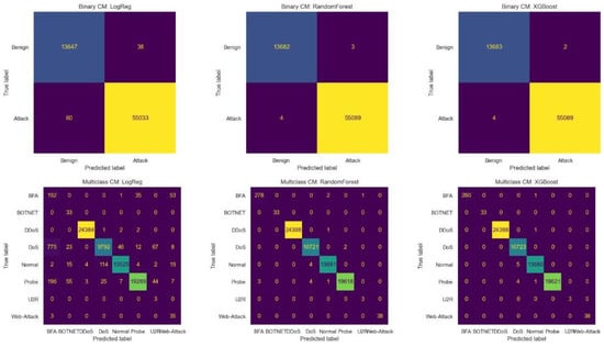
Figure 4.
Confusion matrices for binary and multi-class classification on the InSDN dataset. XGBoost giving the most consistent multi-class results, accurately classifying both majority and minority attack categories.
The winner Table 10 results showed that XGB won all metrics for both binary and multi-classifications.
Table 10.
Winner per metric combined results.
4.10. Hyperparameter Tuning Setup
The hyperparameter optimization process was conducted using RandomizedSearchCV in combination with StratifiedKFold cross-validation, and evaluated using the ROC-AUC score as the primary metric through the use of make_scorer. Figure 5 presents the performance comparison of three binary classification models LR, RF and XGB after hyper-parameter tuning. The evaluation metrics include Accuracy, Precision, Recall, F1 Score, and ROC-AUC, which collectively assess the models’ predictive capabilities. Logistic Regression achieved an accuracy of 0.998459, with nearly identical precision, recall, and F1 scores, indicating consistent performance. Its ROC-AUC score of 0.999403 reflects strong class separation. RF outperformed LogReg with an accuracy of 0.999869 and a near-perfect ROC-AUC of 0.999995, demonstrating its robustness. XGB yielded the highest performance across all metrics, with an accuracy of 0.999927 and a ROC-AUC of 0.999998, indicating almost perfect classification. Figure 6 presents the performance evaluation of three ML models after hyperparameter tuning for a multi-class classification task. The table reports five key metrics: Accuracy, Precision, Recall, F1 Score, and ROC-AUC. LR achieved an accuracy of 0.979863, with a precision of 0.991647 and an F1 score of 0.984817, indicating solid performance but slightly lower than the ensemble models. RF demonstrated near-perfect results, with an accuracy of 0.999753 and a ROC-AUC of 0.999990, reflecting its strong generalization across multiple classes. XGB outperformed all models, achieving the highest scores across all metrics, including a perfect ROC-AUC of 1.000000. These results highlight the effectiveness of hyperparameter tuning in optimizing model performance, particularly for complex multi-class classification tasks, ensemble models, in enhancing binary classification performance and reinforce the superiority of ensemble methods like XGB in handling high-dimensional, real-time data streams in intelligent transportation systems.
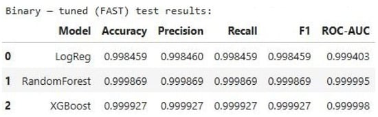
Figure 5.
Hyper parameter-Tuned Results for Binary Classification.
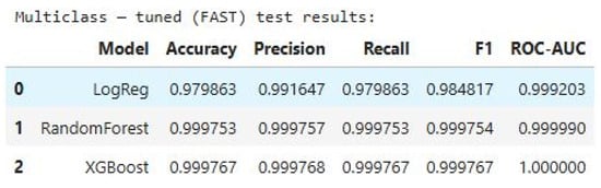
Figure 6.
Hyperparameter-Tuned Results for Multi-Class Classification.
The confusion matrices shown are produced after hyper-parameter tuning of all models and include both raw counts and row-normalized (per-class) views to account for class-size effects.
Figure 7 illustrate the binary classification results on the InSDN dataset after hyper-parameter tuning. Each matrix clearly shows the counts of correctly and incorrectly classified instances for benign and attack traffic. After tuning, all three models, LR, RF &XGB achieved perfect separation, with every benign instance classified as benign and every attack instance classified as attack. The raw count matrices demonstrate that LogReg misclassified a small number of instances (e.g., 40 benign → attack and 66 attack → benign), whereas RF and XGB reduce these errors to near-zero (RF: 3 benign → attack and 6 attack → benign; XGB: 3 benign → attack and 2 attack → benign). In row-normalized form all three models display approximately 100% per-class recall, confirming that hyper-parameter tuning produced highly robust separation between benign and malicious traffic at the binary level. These results confirm that hyper-parameter optimization significantly enhances model reliability, particularly for tree-based models, and demonstrates the feasibility of achieving complete robustness in binary anomaly detection for SDN environments.
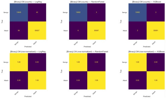
Figure 7.
Confusion matrices after hyper-parameter tuning (binary classification) on the InSDN dataset (Benign vs Attack). Top row: raw counts illustrating absolute misclassification numbers. Bottom row: row-normalized confusion matrices (per-class recall), showing 100% recall for both classes across models after tuning.
Figure 8 illustrate the multi-class classification results on the InSDN dataset after hyper-parameter tuning. This shows the results for eight traffic categories (BFA, Botnet, ddos, dos, normal, probe, U2R, web attack) evaluated with LR, RF and XGB. The top row of subplots shows absolute counts (raw prediction numbers) and the bottom row shows row-normalized matrices. LR showed noticeable improvements compared to the untuned model, correctly classifying most majority classes with strong accuracies such as normal (0.99), probe (0.99), ddos (1.00), and web attack (0.89). However, it still exhibited some confusion, particularly between BFA (0.70 correctly classified, with 0.19 misclassified as web attack) and dos (0.93 correctly classified, with 0.06 misclassified as ddos). In contrast, RF achieved perfect results across all categories, consistently classifying both majority and minority classes with almost no confusion (e.g.,BFA: 0.99, normal: 1.00, probe: 1.00). XGB further improved performance, delivering perfect separation for all classes (1.00 across the diagonal) including rare attacks such as botnet, U2R, and web attack. These results highlight the effectiveness of hyper-parameter tuning, which eliminated the residual misclassifications observed earlier, particularly for tree-based models, and enabled XGB to achieve flawless multi-class classification performance.
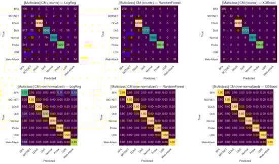
Figure 8.
Confusion matrices after hyper-parameter tuning (multi-class classification) on the InSDN dataset. Top row: raw counts for each model (Logistic Regression, Random Forest, XGBoost). Bottom row: row-normalized confusion matrices (per-class recall). The row-normalized plots emphasize per-class detection performance and reveal that Random Forest and XGBoost achieve near-perfect per-class recall after tuning.
4.11. SHAP Analysis Summary for Feature Interpretability
The SHAP analysis for binary classification provides valuable insights into feature importance and impact distribution, especially in differentiating between benign and malicious network traffic, as shown in Figure 9. The XGB model showcase the top 20 influential features, which illustrate their distribution across prediction outcomes. This helps identify whether specific features consistently influence decisions towards benign or attack classifications, while the colour coding (ranging from blue for low values to red for high values) further clarifies the varying impact of feature values. In multi-class analysis, as shown in Figure 10, SHAP generates separate violin plots for each attack category, offering a detailed view of feature importance for identifying specific attack types such as normal, dos, ddos, and probe. This breakdown not only highlights essential features for distinguishing between various attacks but also illustrates how the model leverages specific feature contributions to recognize different attack patterns, providing a clearer contrast between malicious activities and normal traffic. Overall, the SHAP analysis significantly enhances model transparency and explainability for security practitioners by elucidating the reasons behind network flow classifications. It corroborates the effectiveness of engineered features in intrusion detection, underscores characteristic patterns that separate attack types from benign traffic, and aids compliance with interpretability requirements in AI-driven security frameworks. These insights contribute to the actionable applicability of the XGB intrusion detection system, reinforcing its value in cybersecurity operations.
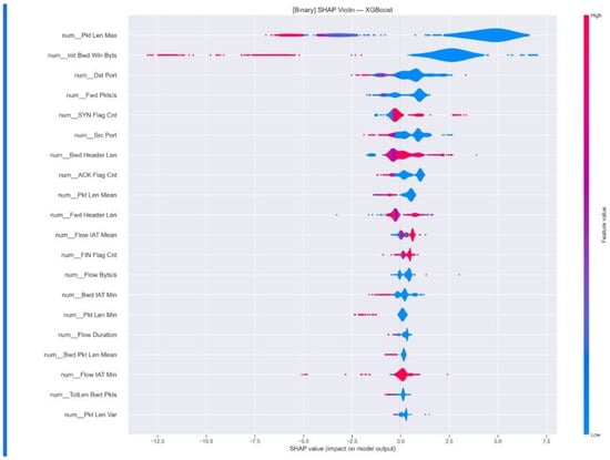
Figure 9.
Binary class after tuned Matrix results.
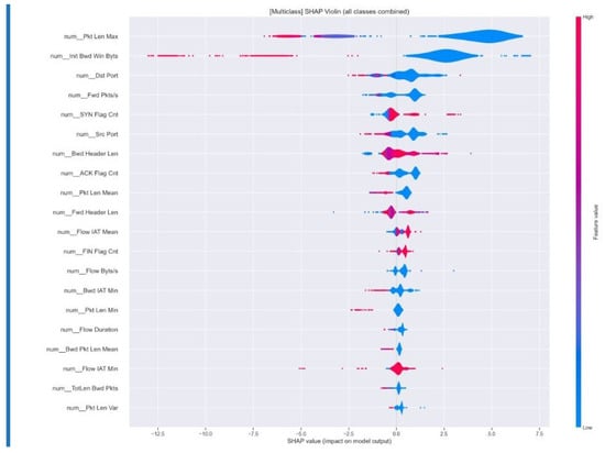
Figure 10.
Multi-class after tuned Matrix results.
Combined ROC Curves (All Models)
The ROC curve analysis demonstrated in Figure 11 exceptional discriminative performance across all three ML models for both binary and multi-class intrusion detection tasks. In the binary classification scenario, all models achieve near-perfect performance with ROC curves tightly hugging the top-left corner of the plot, indicating excellent true positive rates with minimal false positives. LR achieves an AUC of 0.9994, while both RF and XGB reach perfect AUC scores of 1.0000, demonstrating their superior ability to distinguish between benign and malicious network traffic. The multi-class results using micro-averaging show similarly outstanding performance, with LR achieving micro and macro AUC scores of 0.9991 and 0.9972, respectively, while both ensemble methods maintain perfect scores of 1.0000 for all metrics. The steep rise of all curves from the origin and their proximity to the ideal classifier line (top-left corner) validate the robustness of the proposed intrusion detection system. These results confirm that ensemble methods, particularly RF and XGB, provide optimal classification performance for network security applications, with the ability to accurately identify various attack types while maintaining extremely low false positive rates critical for practical deployment in cybersecurity environments.
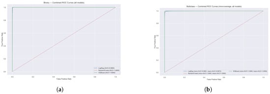
Figure 11.
Combined ROC curves for ALL models (Binary + Multiclass). (a) Binary:Combined ROC Curves (all models); (b) Multiclass:Combined ROC Curves (micro-average, all models).
The offline development and evaluation of ML models demonstrated that ensemble-based classifiers XGB, achieved near-perfect performance in SDN anomaly detection. With accuracy scores exceeding 99.95% and perfect precision and recall values across both normal and attack classes, these models proved highly effective in identifying network anomalies with minimal false positives or negatives. These results confirm the suitability of ensemble learning approaches for offline training in SDN security contexts and lay a strong foundation for real-time integration into streaming frameworks such as Apache Kafka in future stages of this work.
5. How SDN Data Processing Cycle Works Using Apache Kafka
In smart cities, intelligent edge environments consist of IoT devices, autonomous vehicles, and local edge servers that generate vast, diverse, and high-frequency SDN traffic. To handle this data efficiently, Apache Kafka serves as the backbone of the proposed anomaly detection pipeline. Kafka producers collect SDN flow records from edge sources and publish them to Kafka topics, while Kafka consumers retrieve this data and forward it to downstream components. This decoupled design enables real-time ingestion, scalable throughput, and low-latency processing, which are essential for intelligent SDN monitoring.
The anomaly detection engine is built on supervised ML models, including ensemble methods such as Random Forest and XGBoost. These models are trained offline using the InSDN dataset and can be deployed for online inference to classify flows as normal or anomalous. Detected threats include botnets, brute force attacks, DDoS, reconnaissance, and web attacks.
Processed outputs are stored in a PostgreSQL time-series database, enabling both historical insight and real-time querying. The visualization layer integrates Grafana and Streamlit: Grafana provides continuous monitoring dashboards for anomaly trends, while Streamlit offers an interactive interface for uploading datasets, testing models, and inspecting predictions.
To ensure scalability and portability, all components are containerized using Docker, and cloud storage is employed for long-term dataset management. This modular architecture allows seamless integration of raw data ingestion, ML-based detection, and real-time visualization, creating a complete framework for secure SDN-based smart city infrastructure. Figure 12 illustrates the data processing cycle and interactions across system components.
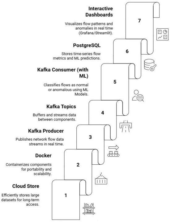
Figure 12.
Kafka-enabled Machine Learning framework in SDN architecture.
After developing and validating the supervised ML models offline using the InSDN dataset, the next step is to demonstrate how these models can be operationalized within a real-time SDN environment. While offline evaluation ensures accuracy and robustness, practical deployment in smart cities requires scalable data ingestion, low-latency processing, and interactive visualization. To address this, Apache Kafka is integrated as the backbone of the proposed data pipeline, enabling seamless streaming, anomaly detection, and monitoring across the entire SDN infrastructure. The following section details how the SDN data processing cycle works using Kafka and supporting tools.
5.1. Kafka-Enabled Machine Learning Framework and System Execution
This section outlines the essential requirements for streaming applications, describes the integration of supporting tools, and explains the offline implementation of the SDN dataset within Kafka environments.
5.2. Requirements Table
Table 11 presents the prototype requirements and their associated components necessary for implementing the proposed Kafka-driven framework.
Table 11.
Prototype requirements and associated components.
5.3. Implementation Workflow
The execution of the proposed Kafka-enabled SDN framework follows a structured workflow, where each component plays a distinct role in enabling real-time anomaly detection and visualization. The key steps are summarized as follows:
- Azure Cloud Storage: Stores SDN datasets in Blob storage, providing scalable and reliable access across environments.
- Dockerized Services: Kafka, Zookeeper, PostgreSQL, and Grafana are deployed in isolated containers to ensure modularity, portability, and scalability.
- Kafka Producer: Streams preprocessed SDN flow records continuously into Kafka topics.
- Kafka Broker: Acts as the central messaging backbone, decoupling ingestion from downstream analytics.
- Kafka Consumer: Consumes records from topics asynchronously and forwards them to the ML pipeline and storage.
- ML Pipeline: Offline-trained models (RF, XGB) classify incoming records as benign or anomalous in real time.
- PostgreSQL Database: Stores structured outputs, including predictions and metadata, for both real-time and historical queries.
- Streamlit Interface: Provides a lightweight interactive frontend on localhost:8501 for model testing, anomaly inspection, and monitoring.
- Grafana Dashboard: Connects to PostgreSQL and Kafka to visualize anomaly trends, class distributions, and system metrics in real time.
5.4. Step 1: Azure Cloud Storage and Dataset Deployment
The Azure Blob Cloud Storage is used and allows scalable and reliable storage of SDN datasets. Docker containers were then utilized to migrate and deploy these datasets across different environments as needed, ensuring portability and consistent data access throughout the pipeline.
5.5. Step 2: Dockerized Kafka–SDN Framework Setup
The proposed Kafka-driven SDN framework was implemented in a fully containerized environment using Docker. The setup consists of Kafka for real-time data streaming, Zookeeper for broker coordination, PostgreSQL for structured and time-series data storage, and Grafana for real-time visualization.
The core infrastructure was deployed using Docker Desktop, which provides a modular and isolated runtime environment for each service, as illustrated in Figure 13 and Figure 14. The command docker-compose up -d was executed to launch all services defined in the docker-compose.yml file in detached mode. Figure 15 displays the list of Docker images deployed as running containers. Each component relies on pre-built images to ensure reproducibility and portability.
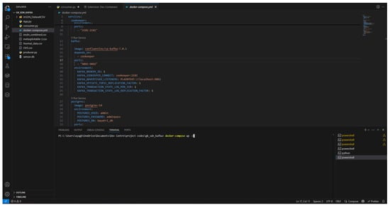
Figure 13.
Execution of Docker compose command in the terminal.
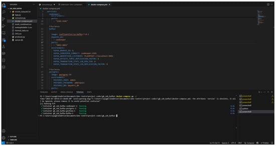
Figure 14.
Successful installations of Zookeeper, Grafana, PostgreSQL, and Kafka.
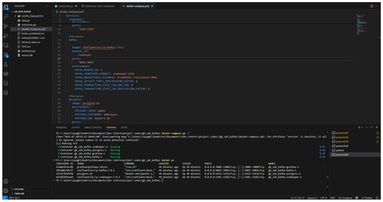
Figure 15.
Results of Docker images list.
Within this framework, Kafka manages real-time data streaming, while Zookeeper coordinates and monitors Kafka brokers. PostgreSQL functions as the backend for structured storage and querying of SDN flow records, and Grafana provides real-time dashboards for monitoring anomalies, system metrics, and traffic distributions. The complete Docker-based architecture, shown in Figure 16, ensures seamless integration, scalability, and continuous monitoring across the data pipeline.
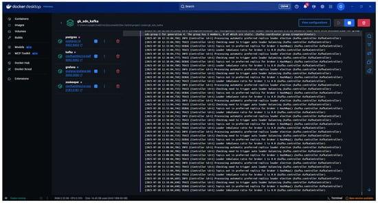
Figure 16.
Docker desktop status.
5.6. Step 3: Real-Time Data Production
The Kafka Producer module, illustrated in Figure 17, is responsible for streaming records from the SDN dataset into designated Kafka topics. This component initiates the real-time machine learning pipeline by ensuring a continuous flow of input data for subsequent processing and anomaly detection when the producer script is executed. As shown in Figure 18, the producer reads preprocessed SDN flow records from the dataset and publishes them to Kafka topics, thereby enabling downstream components such as consumers and ML models to operate on a live data stream.
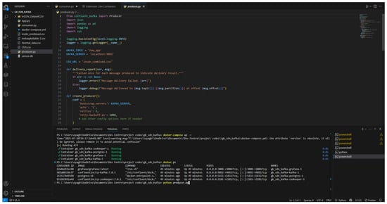
Figure 17.
Kafka producer reads the SDN dataset.
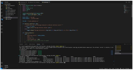
Figure 18.
Kafka producer reads from the SDN dataset and streams the data into defined Kafka topics for downstream processing.
5.7. Step 4: Live Monitoring with Streamlit Application
A Streamlit-based web interface was deployed to provide real-time monitoring of the Kafka consumer output and machine learning predictions, as illustrated in Figure 19 and Figure 20. The application runs locally on localhost:8501 and offers an interactive dashboard that displays performance metrics, anomaly detection results, and class distributions. This interface enables immediate inspection of predictions and system behavior, thereby supporting both research experimentation and operational usability within the proposed framework.
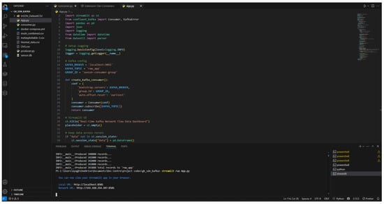
Figure 19.
Streamlit command execution.
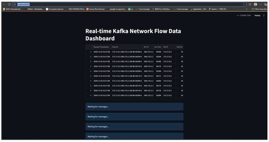
Figure 20.
SDN live analysis: Streamlit web interface (localhost:8501) visualizes the live output of the Kafka consumer and real-time anomaly detection model.
5.8. Step 5: Consumer Execution and Logging
Kafka consumer services are executed in parallel to continuously retrieve messages from Kafka topics, apply real-time ML models, and log the results, as illustrated in Figure 21. The consumer processes each incoming SDN flow record, classifies it using the deployed models, and writes both predictions and system logs into PostgreSQL. As shown in Figure 22, database tables are created programmatically to match the schema of the SDN dataset, where column headers are automatically mapped, enabling structured storage of streaming outputs for subsequent querying and analysis.
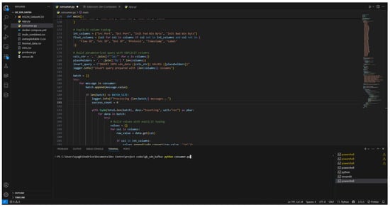
Figure 21.
Kafka consumer processes incoming messages.
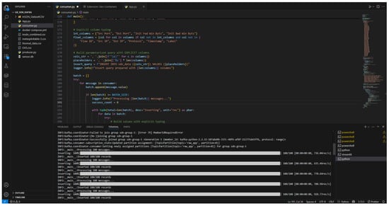
Figure 22.
Kafka consumer logs results into PostgreSQL: The system dynamically creates PostgreSQL tables using column headers from the SDN dataset and uploads streaming outputs for structured querying.
5.9. Step 6: Database Integration and Grafana Visualization Tools
The streaming outputs are persistently stored in PostgreSQL, as illustrated in Figure 23, to support structured analytics and historical querying. Tables are dynamically configured to align with the features and labels of the SDN dataset, ensuring compatibility with downstream tools. Grafana is integrated with PostgreSQL to provide real-time dashboards, enabling the visualization of anomaly trends, traffic class distributions, and system performance metrics. This integration allows continuous monitoring of SDN traffic and enhances operational intelligence through interactive and customizable visual interfaces.
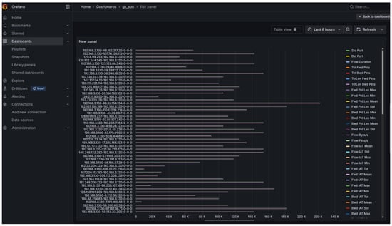
Figure 23.
Grafana dashboards visualize key metrics such as label distribution.
Grafana dashboards, as shown in Figure 24, were created to visualize key metrics such as anomaly counts, class-wise label distribution, and time-based activity trends. The visualizations help interpret the streaming output and ML predictions, highlighting suspicious behaviour patterns or outliers in network traffic.
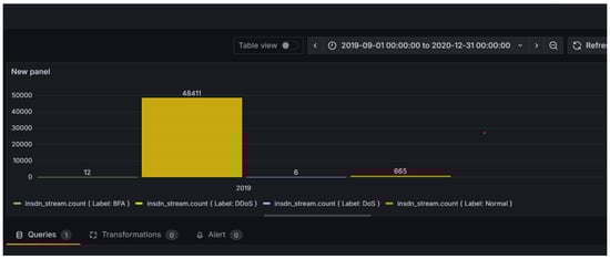
Figure 24.
Grafana dashboards visualize key metrics such as label distribution, anomaly counts, and real-time data trends from PostgreSQL.
5.10. Step 7: Kafka-Enabled Machine Learning Framework Status
Figure 25 presents the operational status of the Kafka-enabled framework. The proposed Kafka-driven SDN streaming model is designed as an extension of the VANET framework and evaluated using the InSDN dataset. The dataset provides a comprehensive set of flow-level features, including source and destination IP addresses, port numbers, flow duration, protocol types, and packet or byte counts attributes that are equally relevant in vehicular environments. In both SDN and VANET scenarios, the primary objective is real-time anomaly detection using network flow data. The machine learning models trained on the InSDN dataset are transferable to vehicular use cases, where abnormal network behaviour can manifest as sudden traffic bursts, spoofed packets, or malicious communication patterns. By reusing the same preprocessing and classification techniques across both domains, the framework ensures consistency, adaptability, and scalability in detecting anomalies across diverse intelligent networking environments.
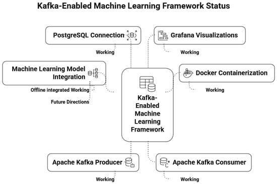
Figure 25.
Kafka-enabled Machine Learning framework status.
5.11. VANET Streaming Framework
The proposed Vehicular Ad-hoc Network (VANET) streaming framework, illustrated in Figure 26, reuses the trained ML models developed using the SDN dataset by mapping vehicular data streams to a comparable format. For example, a vehicle’s data stream published on Kafka topics is structured to match the flow format used in the SDN dataset. This alignment enables seamless anomaly classification using previously trained models, demonstrating the adaptability and extensibility of the Kafka-driven architecture across heterogeneous network domains. In particular, the framework extends into a secure Software-Defined Vehicular Networking (SDVN) paradigm, specifically designed for deployment in intelligent edge environments where low latency, trust, and resilience are critical requirements for intelligent transportation systems.
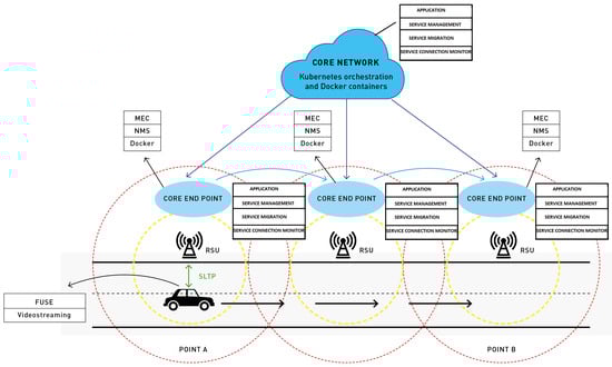
Figure 26.
Implementation scenario: MEC in core end point.
Table 12 presents a comparative mapping between traditional SDN dataset features and their corresponding representations in VANET Kafka streams. This mapping illustrates how conventional network monitoring metrics are adapted for real-time vehicular environments. For instance, flow duration, which is explicitly recorded in SDN datasets, is derived in VANETs from sensor timestamps that capture vehicle movement events. Similarly, packet and byte counts are obtained from vehicle telemetry streams that report communication metrics in real time. Source and destination IP addresses in SDN are mapped to identifiers of On-Board Units (OBUs) and Road-Side Units (RSUs) in VANETs, reflecting the unique, decentralized architecture of vehicular networks. Port numbers, which in SDN are used for flow identification, correspond to network channel mappings in VANETs, denoting logical or physical communication paths between vehicles and infrastructure. The protocol type feature, typically representing TCP or UDP in SDN, is substituted with vehicular communication protocols such as Dedicated Short-Range Communications (DSRC) or Cellular Vehicle-to-Everything (C-V2X). Timestamps are preserved in both systems but, in VANETs, are associated with streaming log times in Kafka, thereby supporting real-time data processing at the edge.
Table 12.
Mapping between SDN dataset features and VANET Kafka streams.
A critical distinction lies in the handling of attack labels. In SDN datasets, labels are manually annotated during dataset preparation. In contrast, within the VANET Kafka streaming framework, labels are predicted dynamically through real-time execution of trained ML models. This shift transforms anomaly detection from a static and offline process into a proactive, scalable, and continuous intrusion detection mechanism.
The overall design illustrates the transition from static, centrally curated SDN datasets to dynamic, distributed vehicular data streams. By embedding this framework as a secure SDVN operating within intelligent edge environments, the system enhances anomaly detection, supports resilience against cyberattacks, and provides scalable real-time analytics. This not only strengthens the adaptability of the Kafka-ML architecture but also advances the vision of secure, intelligent transportation systems capable of meeting the demands of next-generation mobility.
6. Conclusions and Future Work
This research presented an end-to-end framework for real-time anomaly detection in Software-Defined Networking (SDN) environments by integrating machine learning models with scalable, containerized streaming architectures in Intelligent Edge Environments (IEEs). Ensemble learning algorithms, including RF, LG, and XGB, were initially trained and evaluated offline using SDN datasets. The models achieved outstanding performance, with XGB demonstrating near-perfect precision, recall, and ROC-AUC scores, confirming its robustness in distinguishing normal and malicious traffic patterns. The implementation workflow leveraged Azure Blob Storage for dataset management and a Dockerized microservices architecture for modular and scalable deployment. Apache Kafka enabled efficient real-time data streaming, while PostgreSQL supported structured storage of predictions. Streamlit and Grafana were incorporated to provide live monitoring and visualization of anomaly trends and system metrics. Importantly, the framework is designed not only to classify incoming flow records in real time but also to address advanced threats, including evasion attacks, SSL/TLS exploits, authentication breaches, and broader system security risks. Beyond SDN, the use case of Vehicular Ad-hoc Networks (VANETs) was explored to demonstrate the adaptability of the proposed Kafka-enabled ML pipeline. By mapping vehicular data streams to SDN-like flow features, the framework extends into secure Software-Defined Vehicular Networking (SDVN), deployed within intelligent edge environments for enhanced resilience, security, and scalability. Overall, this work demonstrates the feasibility and effectiveness of deploying a robust, offline anomaly detection system in SDN-enabled IEEs. Future research directions include extending the pipeline to support adaptive learning mechanisms, ingestion of real-time data, and integration with distributed threat intelligence systems to enable proactive, collaborative defence across next-generation network infrastructures.
Author Contributions
Conceptualization, software implementation, writing—review and editing, G.K.; Conceptualization, methodology, supervision, writing—review and editing, G.M. Review, J.C. All authors have read and agreed to the published version of the manuscript.
Funding
This research received no external funding.
Data Availability Statement
The original contributions presented in this study are included in the article. Further inquiries can be directed to the corresponding author.
Conflicts of Interest
The authors declare no conflicts of interest.
Correction Statement
This article has been republished with a minor correction to the Data Availability Statement. This change does not affect the scientific content of the article.
References
- Karthick, G.; Mapp, G. Developing a Secure Service Ecosystem to Implement the Intelligent Edge Environment for Smart Cities. Future Internet 2024, 16, 317. [Google Scholar] [CrossRef]
- Elassy, M.; Al-Hattab, M.; Takruri, M.; Badawi, S. Intelligent transportation systems for sustainable smart cities. Transp. Eng. 2024, 16, 100252. [Google Scholar] [CrossRef]
- Dave, R.; Seliya, N.; Siddiqui, N. The benefits of edge computing in healthcare, smart cities, and IoT. arXiv 2021, arXiv:2112.01250. [Google Scholar] [CrossRef]
- Minh, Q.N.; Nguyen, V.H.; Quy, V.K.; Ngoc, L.A.; Chehri, A.; Jeon, G. Edge computing for IoT-enabled smart grid: The future of energy. Energies 2022, 15, 6140. [Google Scholar] [CrossRef]
- Karthick, G.; Mapp, G.; Crowcroft, J. Building an Intelligent Edge Environment to Provide Essential Services for Smart Cities. In Proceedings of the 18th Workshop on Mobility in the Evolving Internet Architecture, MobiArch’23, Madrid, Spain, 6 October 2023; pp. 13–18. [Google Scholar] [CrossRef]
- Dantas Silva, F.S.; Neto, E.; Santos, C.; Almeida, T.; Silva, I.; Neto, A.V. Evolving Fast Innovation in Next-Generation Networking Through Flexible and Customized Softwarization and Slicing Capabilities. In Proceedings of the 2020 IEEE Conference on Network Function Virtualization and Software Defined Networks (NFV-SDN), Leganes, Spain, 10–12 November 2020; pp. 188–193. [Google Scholar] [CrossRef]
- Sanapala, S.; Reddy, D.D.; Chowdary, G.L.; Vikyath, K. Machine Learning Based DDoS Attack Detection in Software Defined Networks (SDN). In Proceedings of the 2023 2nd International Conference on Edge Computing and Applications (ICECAA), Namakkal, India, 19–21 July 2023; pp. 1124–1126. [Google Scholar] [CrossRef]
- Boussaoud, K.; En-Nouaary, A.; Ayache, M. Adaptive Congestion Detection and Traffic Control in Software-Defined Networks via Data-Driven Multi-Agent Reinforcement Learning. Computers 2025, 14, 236. [Google Scholar] [CrossRef]
- Huang, W.; Liu, H.; Li, Y.; Ma, L. ERA-MADDPG: An Elastic Routing Algorithm Based on Multi-Agent Deep Deterministic Policy Gradient in SDN. Future Internet 2025, 17, 291. [Google Scholar] [CrossRef]
- Apache Kafka. 2024. Available online: https://kafka.apache.org/ (accessed on 13 July 2025).
- Moon, J.H.; Shine, Y.T. A Study of Distributed SDN Controller Based on Apache Kafka. In Proceedings of the 2020 IEEE International Conference on Big Data and Smart Computing (BigComp), Busan, Republic of Korea, 19–22 February 2020; pp. 44–47. [Google Scholar] [CrossRef]
- Hamedani, A.F.; Aziz, M.; Wieder, P.; Yahyapour, R. Big Data Framework to Detect and Mitigate Distributed Denial of Service(DDoS) Attacks in Software-Defined Networks (SDN). In Proceedings of the 2023 3rd International Conference on Electrical, Computer, Communications and Mechatronics Engineering (ICECCME), Tenerife, Spain, 19–21 July 2023; pp. 1–6. [Google Scholar] [CrossRef]
- Majd Latah, L.T. Towards an Efficient Anomaly-Based Intrusion Detection for Software-Defined Networks. IET Netw. 2018, 7, 453–459. [Google Scholar] [CrossRef]
- El Sayed, M.S.; Le-Khac, N.A.; Azer, M.A.; Jurcut, A.D. A flow-based anomaly detection approach with feature selection method against ddos attacks in sdns. IEEE Trans. Cogn. Commun. Netw. 2022, 8, 1862–1880. [Google Scholar] [CrossRef]
- Dawoud, A.; Shahristani, S.; Raun, C. Deep learning and software-defined networks: Towards secure IoT architecture. Internet Things 2018, 3–4, 82–89. [Google Scholar] [CrossRef]
- Hamarshe, A.; Ashqar, H.I.; Hamarsheh, M. Detection of DDoS Attacks in Software Defined Networking Using Machine Learning Models. In Proceedings of the 2023 International Conference on Advances in Computing Research (ACR’23), Orlando, FL, USA, 8–10 May2023; pp. 640–651. [Google Scholar]
- Yu, H.; Yang, W.; Cui, B.; Sui, R.; Wu, X. Renyi entropy-driven network traffic anomaly detection with dynamic threshold. Cybersecurity 2024, 7, 64. [Google Scholar] [CrossRef]
- Varalakshmi, I.; Thenmozhi, M. entropy based earlier detection and mitigation of ddos attack using stochastic method in sdn iot. Meas. Sens. 2025, 39, 101873. [Google Scholar] [CrossRef]
- Ahmed, N.; Ngadi, A.B.; Sharif, J.M.; Hussain, S.; Uddin, M.; Rathore, M.S.; Iqbal, J.; Abdelhaq, M.; Alsaqour, R.; Ullah, S.S.; et al. Network threat detection using machine/deep learning in SDN-based platforms: A comprehensive analysis of state-of-the-art solutions, discussion, challenges, and future research direction. Sensors 2022, 22, 7896. [Google Scholar] [CrossRef] [PubMed]
- Vyas, S.; Tyagi, R.K.; Jain, C.; Sahu, S. Literature review: A comparative study of real-time streaming technologies and apache kafka. In Proceedings of the 2021 Fourth International Conference on Computational Intelligence and Communication Technologies (CCICT), Sonepat, India, 3 July 2021; pp. 146–153. [Google Scholar]
- Chen, W.; Milosevic, Z.; Rabhi, F.A.; Berry, A. Real-Time Analytics: Concepts, Architectures, and ML/AI Considerations. IEEE Access 2023, 11, 71634–71657. [Google Scholar] [CrossRef]
- Padmanaban, K.; Ganesh Babu, T.R.; Karthika, K.; Pattanaik, B.; K, D.; Srinivasan, C. Apache Kafka on Big Data Event Streaming for Enhanced Data Flows. In Proceedings of the 2024 8th International Conference on I-SMAC (IoT in Social, Mobile, Analytics and Cloud) (I-SMAC), Kirtipur, Nepal, 3–5 October 2024; pp. 977–983. [Google Scholar] [CrossRef]
- Kazi, B.U.; Islam, M.K.; Siddiqui, M.M.H.; Jaseemuddin, M. A Survey on Software Defined Network-Enabled Edge Cloud Networks: Challenges and Future Research Directions. Network 2025, 5, 16. [Google Scholar] [CrossRef]
- da Silva Ruffo, V.G.; Brandão Lent, D.M.; Komarchesqui, M.; Schiavon, V.F.; de Assis, M.V.O.; Carvalho, L.F.; Proença, M.L. Anomaly and intrusion detection using deep learning for software-defined networks: A survey. Expert Syst. Appl. 2024, 256, 124982. [Google Scholar] [CrossRef]
- Janabi, A.H.; Kanakis, T.; Johnson, M. Survey: Intrusion detection system in software-defined networking. IEEE Access 2024, 12, 164097–164120. [Google Scholar] [CrossRef]
- Shen, Y.; Jeong, J.; Jun, J.; Oh, T.; Baek, Y. ecmac: Edge assisted cluster-based mac protocol in software defined vehicular networks. IEEE Trans. Veh. Technol. 2024, 73, 13738–13750. [Google Scholar] [CrossRef]
- Dias, D.; Luís, M.; Rito, P.; Sargento, S. A Software Defined Vehicular Network Using Cooperative Intelligent Transport System Messages. IEEE Access 2024, 12, 93152–93170. [Google Scholar] [CrossRef]
- Paranthaman, V.V.; Ghosh, A.; Mapp, G.; Iniovosa, V.; Shah, P.; Nguyen, H.X.; Gemikonakli, O.; Rahman, S. Building a Prototype VANET Testbed to Explore Communication Dynamics in Highly Mobile Environments. In Proceedings of the Testbeds and Research Infrastructures for the Development of Networks and Communities, Hangzhou, China, 14–15 June 2016; pp. 81–90. [Google Scholar]
- Ramirez, J.; Ezenwigbo, O.A.; Karthick, G.; Trestian, R.; Mapp, G. A new service management framework for vehicular networks. In Proceedings of the 2020 23rd Conference on Innovation in Clouds, Internet and Networks and Workshops (ICIN), Paris, France, 24–27 February 2020; pp. 162–164. [Google Scholar] [CrossRef]
- Khalid, H.Y.I.; Aldabagh, N.B.I. A survey on the latest intrusion detection datasets for software defined networking environments. Eng. Technol. Appl. Sci. Res. 2024, 14, 13190–13200. [Google Scholar] [CrossRef]
- Elsayed, M.S.; Le-Khac, N.A.; Jurcut, A.D. InSDN: A novel sdn Intrusion dataset. IEEE Access 2020, 8, 165263–165284. [Google Scholar] [CrossRef]
Disclaimer/Publisher’s Note: The statements, opinions and data contained in all publications are solely those of the individual author(s) and contributor(s) and not of MDPI and/or the editor(s). MDPI and/or the editor(s) disclaim responsibility for any injury to people or property resulting from any ideas, methods, instructions or products referred to in the content. |
© 2025 by the authors. Licensee MDPI, Basel, Switzerland. This article is an open access article distributed under the terms and conditions of the Creative Commons Attribution (CC BY) license (https://creativecommons.org/licenses/by/4.0/).