Article

Detection and Mitigation in IoT Ecosystems Using oneM2M Architecture and Edge-Based Machine Learning

Department of Electrical Engineering, National Formosa University, Yunlin 632301, Taiwan
*
Author to whom correspondence should be addressed.
Future Internet 2025, 17(9), 411; https://doi.org/10.3390/fi17090411
Submission received: 31 July 2025 / Revised: 1 September 2025 / Accepted: 5 September 2025 / Published: 8 September 2025
(This article belongs to the Special Issue DDoS Attack Detection for Cyber–Physical Systems)

Abstract

Distributed denial-of-service (DDoS) attacks are a prevalent threat to resource-constrained IoT deployments. We present an edge-based detection and mitigation system integrated with the oneM2M architecture. By using a Raspberry Pi 4 client and five Raspberry Pi 3 attack nodes in a smart-home testbed, we collected 200,000 packets with 19 features across four traffic states (normal, SYN/UDP/ICMP floods), trained Decision Tree, 2D-CNN, and LSTM models, and deployed the best model on an edge computer for real-time inference. The edge node classifies traffic and triggers per-attack defenses on the device (SYN cookies, UDP/ICMP iptables rules). On a held-out test set, the 2D-CNN achieved 98.45% accuracy, outperforming the LSTM (96.14%) and Decision Tree (93.77%). In end-to-end trials, the system sustained service during SYN floods (time to capture 200 packets increased from 5.05 s to 5.51 s after enabling SYN cookies), mitigated ICMP floods via rate limiting, and flagged UDP floods for administrator intervention due to residual performance degradation. These results show that lightweight, edge-deployed learning with targeted controls can harden oneM2M-based IoT systems against common DDoS vectors.

1. Introduction

The Internet of Things (IoT) is an emerging communication paradigm that enables heterogeneous devices to connect through sensors for data collection and remote control. It has been widely applied in fields such as environmental monitoring, smart buildings, vehicular networks, healthcare, and Industry 4.0 applications [1,2,3]. IoT applications can be broadly categorized into two types—those requiring low latency and high-speed communication (e.g., vehicular networks) and those involving massive sensor data processing (e.g., smart factories), both of which are tightly integrated with 5G technology. The IoT architecture generally consists of three layers—the perception layer, the network layer, and the application layer [4]. However, due to cost constraints, most IoT devices and gateways lack sufficient storage and computational power to support conventional security software, such as antivirus programs, intrusion detection systems (IDS), or intrusion prevention systems (IPS), resulting in significant cybersecurity vulnerabilities [5]. As the number of connected devices and the frequency of data transmission continue to grow, the risk of cyberattacks also increases. Once compromised, attackers can steal personal data, disseminate spam, or leverage infected devices to launch DDoS attacks [6].
A notable real-world example is the 2015 Ukraine power grid attack, where attackers deployed the “Black Energy” malware via phishing emails to infiltrate operator systems, remotely shut down breakers, and subsequently launch a DDoS attack, causing a large-scale blackout [7]. DDoS attacks are among the most common threats in IoT environments and are typically classified into bandwidth-exhaustion and resource-exhaustion attacks. The former includes techniques such as UDP floods and ICMP floods [8,9,10,11]. While traditional defenses rely on firewalls and IDS, these methods often fall short in identifying more complex and evolving attack vectors. In recent years, machine learning and deep learning techniques have been increasingly adopted for more intelligent intrusion detection [12]. In this study, we propose a multi-model detection framework that combines Decision Tree (DT) [13,14,15,16], Convolutional Neural Network (CNN) [17,18,19], and long short-term memory (LSTM) models to analyze Layer 3 and Layer 4 network traffic. In addition to packet features, the system also integrates CPU usage, memory status, and network traffic conditions as labeled features to enhance classification accuracy. The proposed model is deployed on an IoT platform based on the oneM2M architecture for real-world validation.
  • We deployed an edge-based DDoS detector tightly integrated with oneM2M, enabling on-device, per-attack responses in a smart-home setting.
  • We combined packet-level features with system signals (CPU/memory/traffic) to improve robustness under resource contention.
  • We provided an efficient 2D-CNN design that achieves 98.45% accuracy with low inference overhead on edge hardware, outperforming LSTM and Decision Tree in our tests.
  • We demonstrated attack-specific mitigations (SYN cookies and iptables rate limits) and quantified end-to-end impact under SYN/UDP/ICMP floods.

2. Related Work

In the last three years, MDPI studies have increasingly moved DDoS detection to the edge/IoT layer to shorten reaction time and avoid backbone congestion. Representative directions include SDN/edge parallelism that distributes detection to edge switches for real-time operation [20], edge–cloud designs that reduce feature complexity yet maintain high accuracy for on-device deployment [21], and mobile edge computing with blockchain that integrates high-accuracy ML detectors and near-source mitigation (e.g., a Transformer reported at 99.78% on CICDDoS2019) [22]. Following this line, our system deploys a lightweight 2D-CNN at the edge and quantifies the window-size–latency trade-off as well as end-to-end behavior and attack-specific mitigation in a real testbed. Complementary to these classical approaches, recent work indicates that hybrid quantum–classical CNNs can improve adversarial robustness and that quantum Born-machine–based QGANs can support data augmentation for minority or hard-to-collect attack patterns; these are promising directions for future extension given current NISQ hardware constraints [23,24].

2.1. oneM2M

oneM2M is a global collaborative initiative established in 2012 with the goal of defining a network-independent, horizontal service layer solution that enables interoperability among various existing Machine-to-Machine (M2M) vertical systems [25,26,27,28]. It is formed by eight of the world’s leading ICT standards development organizations, including ARIB (Japan), ATIS (USA), CCSA (China), ETSI (Europe), TIA (USA), TSDSI (India), TTA (Korea), and TTC (Japan). In addition to these founding members, more than 200 partner organizations and members have contributed to the initiative, including prominent industry leaders such as IBM, Cisco, Intel, Samsung, AT&T, and Ericsson.
The communication protocol adopted by oneM2M is Representational State Transfer (REST), a concept introduced and defined by Roy Thomas Fielding in his doctoral dissertation [29,30]. REST communicates solely through the exchange of resource states. Typically, the two communicating parties are referred to as the client (consumer) and the server (provider). The client initiates a request to the server, which then responds with a corresponding reply. Both the request and the response are strictly based on the exchange of resource representations. Any communication method that adheres to these constraints is referred to as RESTful.

2.2. DDoS

A DDoS attack is an evolved form of the Denial of Service (DoS) attack [31,32,33,34]. DDoS attacks are generally classified into two major categories: network bandwidth exhaustion and system resource exhaustion. These attacks are often carried out using a botnet—a network of compromised computers infected with malware. The infected devices, known as bots or zombie computers, receive commands from an attacker and simultaneously launch coordinated attacks against a single target. This overwhelms the victim’s network and system resources, rendering services unavailable to legitimate users. From the user’s perspective, the server appears to malfunction or crash, hence the term “denial of service.” When such an attack is executed by a distributed network of infected devices, it is referred to as a DDoS attack, as illustrated in Figure 1.
To build a botnet, attackers must first infect victim computers with malware. This is typically achieved by exploiting system vulnerabilities, backdoors, spam emails, malicious links, or similar techniques. Once a computer is infected, it may act as a launching point to propagate the malware to other machines, expanding the botnet. Infected machines then attempt to establish communication with the botnet’s command-and-control (C&C) server, which is used by the attacker to manage the network.

2.3. LSTM

LSTM [35,36] is a type of RNN. Traditional neural network models do not inherently account for the sequential nature of data, and time-series information is typically treated as independent features for prediction or classification tasks. In contrast, RNNs are specifically designed to handle sequential data, making them well-suited for applications such as speech recognition and stock price prediction.
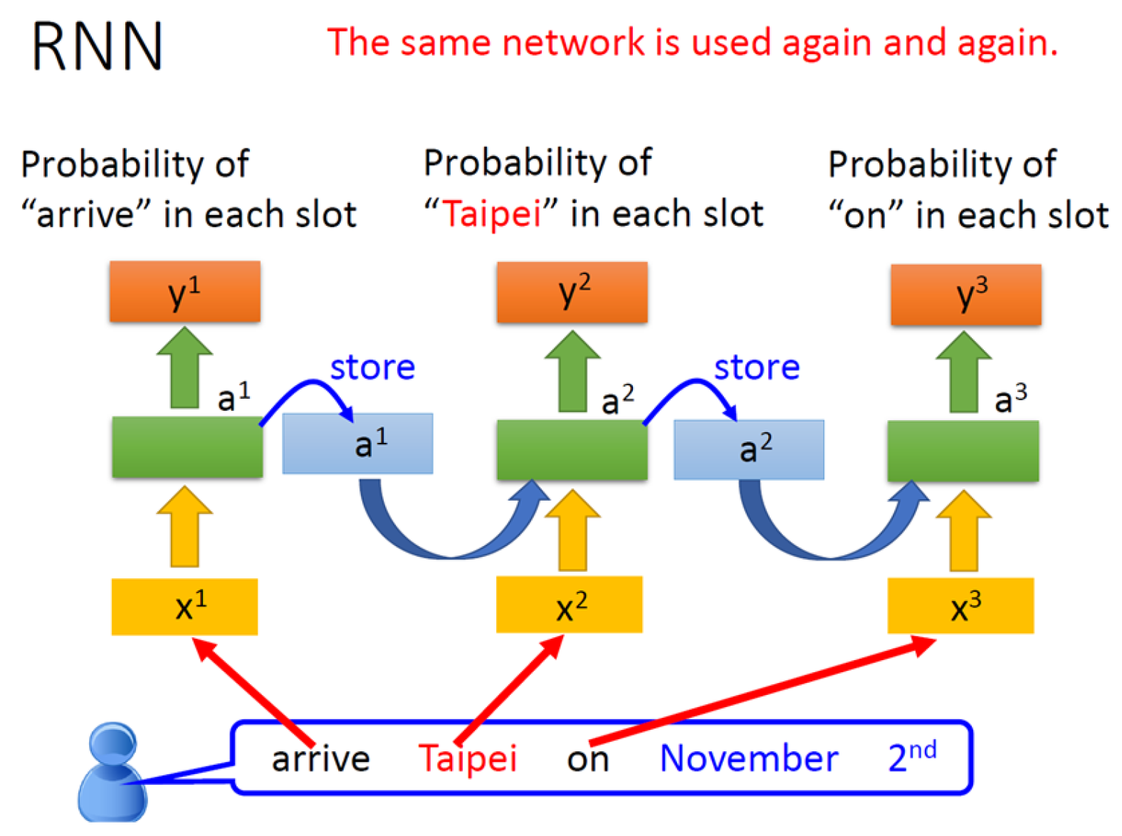
The architecture of a basic RNN model is illustrated in Figure 2, which presents a sentence interpretation example. In this figure, the input x1 = “arrive” is represented as a vector and passed into the neural network, producing a1 as the output from the hidden layer. The output y1 then indicates the probability that the word “arrive” belongs to a particular slot. The hidden state a1 is stored in memory. Next, the word “Taipei” becomes the new input, and the hidden layer computes a2 by considering both the current input “Taipei” and the stored hidden state a1. This process continues iteratively to generate y2, and so on.
LSTM is a type of RNN with similar principles but a more complex structure. Its most important design is the “conveyor belt,” i.e., the vector Ct, which allows past information to be carried over to the next time step and thus effectively alleviates the vanishing gradient problem in simple RNNs. Figure 3 shows a simplified LSTM architecture. Each neuron in an LSTM has four inputs and one output—the input gate, forget gate, new value ( C ~ t), and output gate as inputs, and the output is ht.

2.4. Recent Baselines and Our Positioning

Recent IoT/edge DDoS studies report strong results on public datasets (e.g., CICDDoS-series and Edge-IIoTset) using RF/CNN/Transformer variants, often under server-grade or controller-assisted setups. Our study targets a oneM2M smart-home testbed with on-device feasibility, where the 2D-CNN attains 98.45% accuracy (Section 4.5). As datasets differ in traffic mix and labeling policies, direct score matching is not strictly comparable; we therefore emphasize deployability (edge inference and short windows) and end-to-end utility (mitigation triggering).

3. Materials and Methods

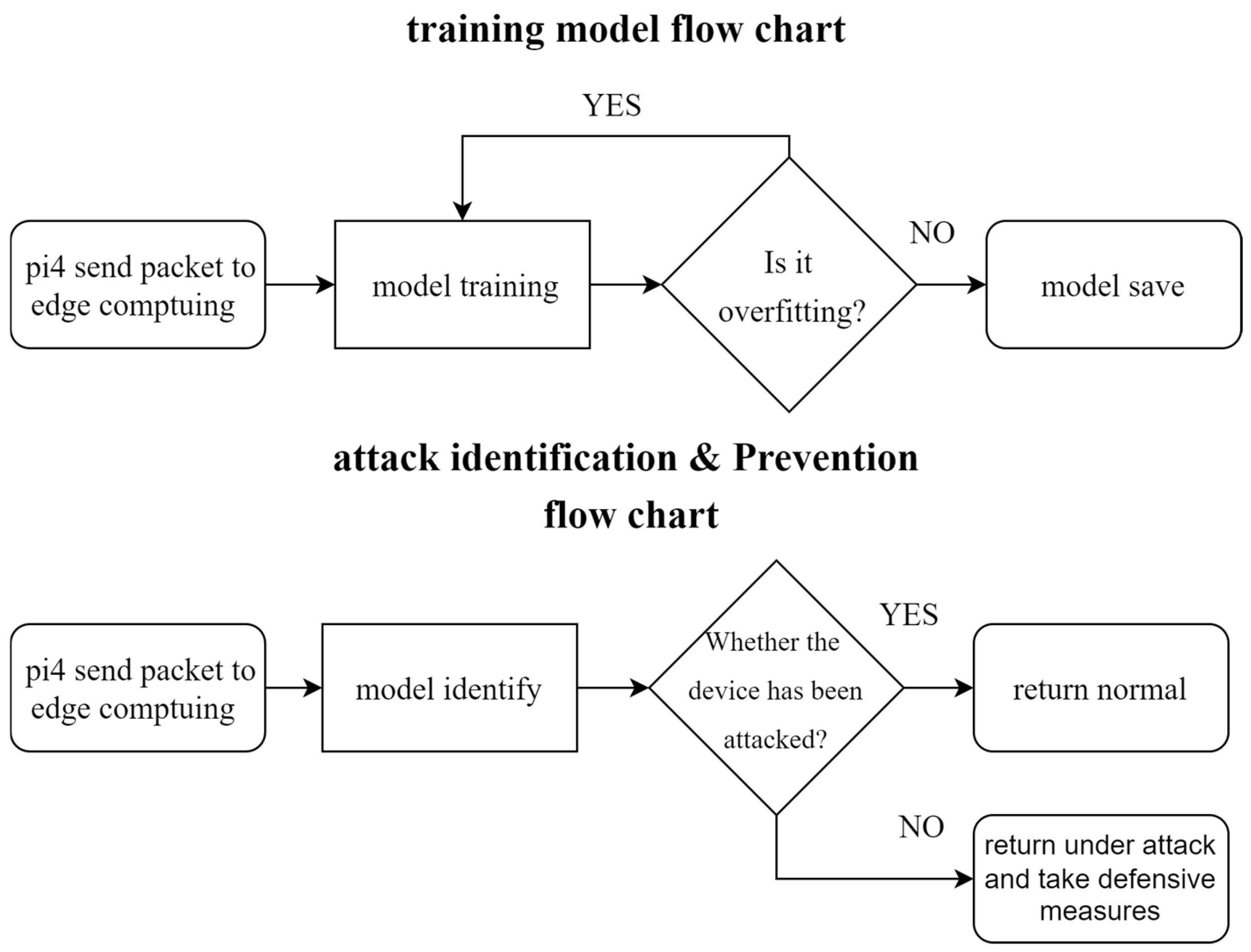
The implementation process is shown in Figure 4. First, the experimental method is to collect the normal types and packet characteristics of each attack and organize them into a dataset. The second step is to train the model, and the third step is to obtain high accuracy on two different test sets, making sure the model does not overfit.
Once the model is built, detection and application can be enabled within the oneM2M IoT application platform. A Raspberry Pi 4 (hereafter referred to as “Pi 4”) serves as a sensing node, corresponding to the MN-AE and MN-CSE components of the oneM2M architecture, storing field data for future use. Five Raspberry Pi 3 are used as attack devices to simulate IoT devices controlled by botnets; edge computing computers are used to set up servers as infrastructure domains and receive incoming data from IP1. The data of Pi 4 is stored, and the packets of IP1 captured by Tshark are received from IP2 and analyzed. Finally, the recognition result is returned to Pi 4 through the socket connection through the trained model, and Pi 4 is made corresponding to the recognition result. defensive measures.

3.1. System Architecture

This study utilizes a total of six Raspberry Pi devices (five Raspberry Pi 3 units and one Raspberry Pi 4, hereafter referred to as Pi 3 and Pi 4, respectively), as illustrated in Figure 5. The Pi 4 serves as the IoT client device for data transmission, equipped with a USB wireless network adapter to facilitate communication with the edge computing computer. The remaining five Pi3 units are configured as DDoS attack nodes.
The experimental environment is based on a smart home model following the oneM2M architecture, as shown in Figure 6. In this setup, IoT sensor nodes are used to collect environmental data and transmit it over a 2.4 GHz Wi-Fi network. The smart home system comprises Arduino boards, sensors, Raspberry Pi devices, a computer, and a smartphone. In the context of the oneM2M architecture, the sensors correspond to ADN-AE (Application Dedicated Node–Application Entity); the Raspberry Pi devices represent both MN-CSE (Middle Node–Common Services Entity) and MN-AE (Middle Node–Application Entity); and the edge computing computer not only collects network packets from the Pi 4 but also uses an additional wireless adapter to receive data transmitted from the Raspberry Pi-based sensors, functioning as the IN-CSE (Infrastructure Node–Common Services Entity). The smartphone, acting as an IN-AE (Infrastructure Node–Application Entity), can remotely control the system via a mobile application.

3.2. Real-Time Detection System Architecture

This study aims to detect DDoS attacks occurring within an internal network and to apply appropriate defense mechanisms based on the type of attack. To achieve this, a controlled DDoS attack environment was constructed. One key advantage of using machine learning and deep learning models lies in their ability to improve DDoS detection accuracy while simultaneously reducing dependence on specific hardware and software environments. Additionally, such models simplify the process of real-time system updates and upgrading detection strategies.
Three algorithms—Decision Tree (DT), Convolutional Neural Network (CNN), and LSTM—were utilized for attack classification in this research. The DDoS attack simulation programs were implemented in Python 3.10.14 and used to launch attacks on the server, including SYN flood, UDP flood, and ICMP flood attacks, as illustrated in the system architecture diagram.
The training dataset for the classification models was collected from the Pi 4 device under both normal and attack conditions, covering four distinct system states. A total of 200,000 packets across 19 feature categories were collected, and feature extraction from these packets yielded approximately 3.8 million data entries.
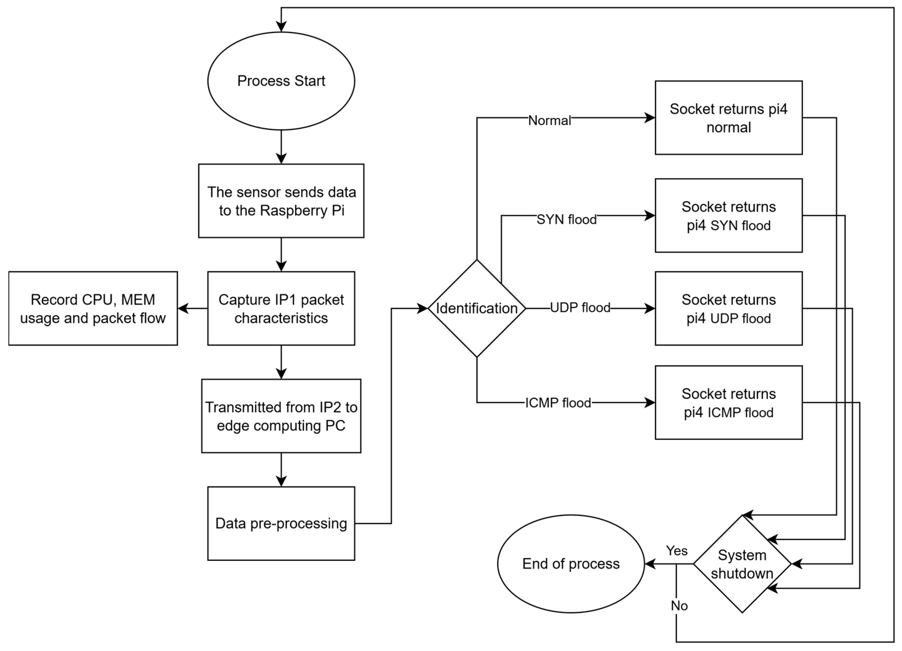
The real-time detection system captures packets transmitted from IP1 and simultaneously logs system metrics from the Pi 4 device, including CPU usage, memory status, and network traffic conditions. This information is then transmitted via IP2 to the edge computing computer, which analyzes the data to determine whether the system is operating normally. If an attack is detected, the edge device sends back the corresponding defense instructions to the Pi 4. The decision-making process is illustrated in Figure 7.

Theory and Rationale

We cast detection as a multi-class classification over traffic states (normal, SYN, UDP, ICMP). Windowed features capture class-specific protocol signals at low latency: (i) SYN floods raise the SYN/ACK–ACK imbalance, reflected in tcp.flags and tcp.dstport; (ii) UDP floods show connectionless bursts with low entropy in udp.dstport/udp.length; and (iii) ICMP floods yield dense echo sequences with monotone icmp.seq_le. These signals align with our feature set (Table 1) and enable separation using lightweight models. Decision Trees leverage information gain to select discriminative attributes, CNNs aggregate local temporal-feature patterns across short windows, and LSTMs model short-range dynamics. Short windows reduce buffering latency and memory, which suits edge devices while still preserving attack-specific patterns.

3.3. Dataset and Model Training

In this study, the Raspberry Pi 4 (Pi 4) is equipped with an additional Wi-Fi USB adapter, enabling it to operate with two IP addresses. The IP address provided by the built-in Wi-Fi interface is referred to as IP1, while the IP address assigned to the external Wi-Fi adapter is referred to as IP2. IP2 is a private IP address that transmits data to the edge computing computer through a proxy to enhance transmission security.
IP1 is connected to a 2.4 GHz Wi-Fi network and is used for transmitting sensor data. While collecting data through IP1, the system simultaneously simulates DDoS attacks targeting IP1. To prevent potential errors in system behavior on the Pi 4 caused by attack-induced resource exhaustion, a separate edge computing PC is employed. This PC connects to a 5 GHz Wi-Fi network and uses IP2 to receive the packets collected from IP1. This setup ensures that packet transmission to the edge device remains unaffected by potential network congestion or delays caused by the attacks. Once the data are processed by the detection model, the results are sent back to the Pi 4. If an attack is detected, corresponding defense actions are triggered. The entire process is illustrated in Figure 8.
In this architecture, the edge computing PC functions as the decision-making node, responsible for attack classification and analysis. The Pi 4 acts as the execution node, carrying out the defense actions issued by the decision-making node.

3.4. Packet Capture and Dataset Construction

The sensing node (ADN-AE in the oneM2M architecture) uses a DHT11 temperature and humidity sensor to monitor environmental conditions. The sensor measures 0–50 °C (±5 °C) and 20–90% RH. Readings are sent every 3 s to the MN-AE, which relays them over 2.4 GHz Wi-Fi to the IN-CSE. Following [5], the dataset was built by capturing packets arriving on IP1 with Tshark on a Pi 4 and forwarding them over IP2 to an edge computer for storage and processing. Tshark, the command-line version of Wireshark on Linux, supports field-level filters, conditional capture, and file export, enabling tailored data collection.
Figure 9 lists the specific parameters used during the experiments.
As summarized in Table 1, the dataset contains a total of 21 fields. The first 19 fields were captured directly by Tshark, while the final two fields were manually labeled—representing the attack label and the attack type category, respectively.

3.5. Model Training

This section presents the training processes for three models—Decision Tree (DT), Convolutional Neural Network (CNN), and LSTM—and compares their experimental results.

3.5.1. Decision Tree (DT)

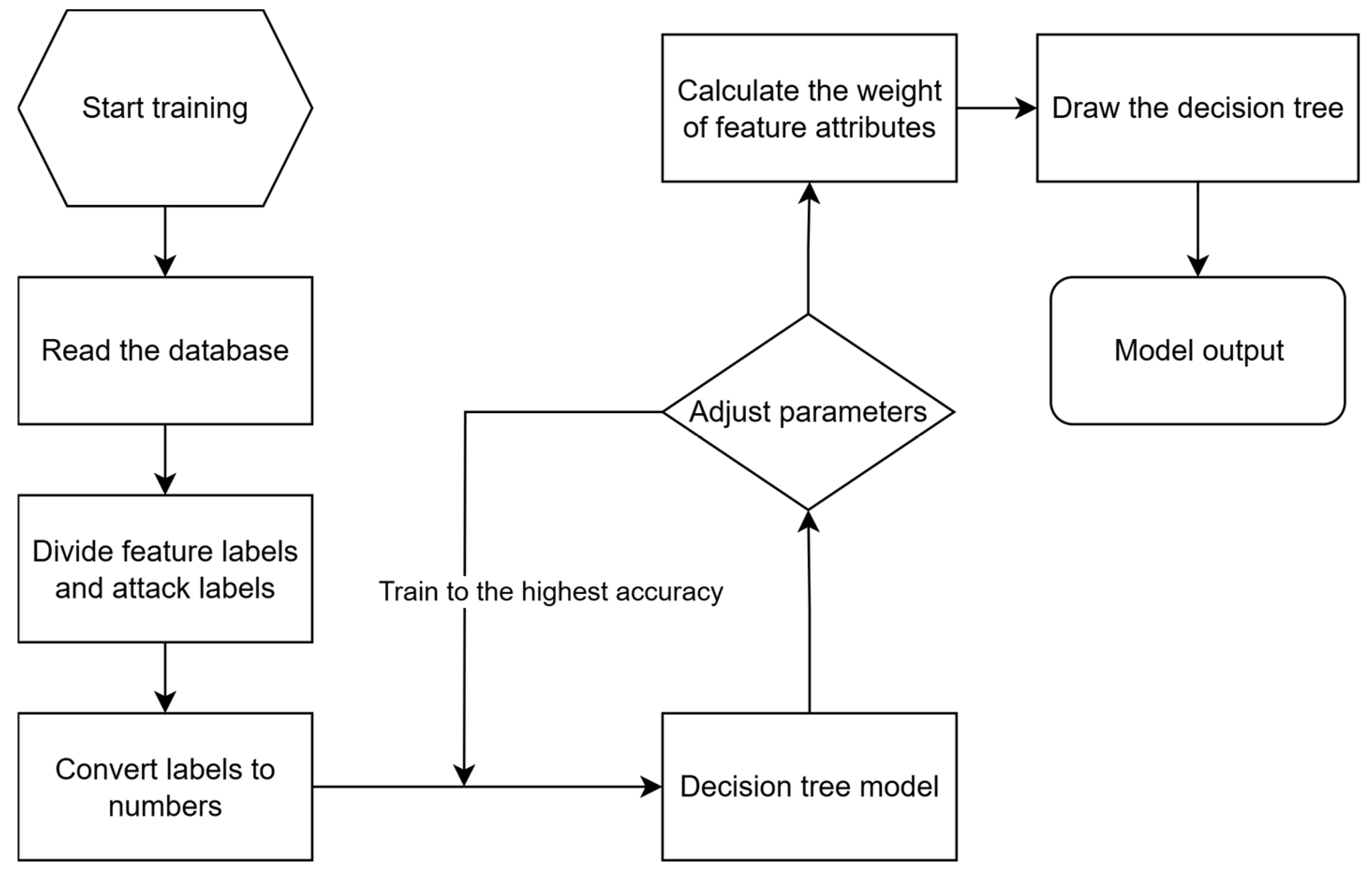
The collected dataset was labeled and preprocessed using the LabelEncoder function from the Scikit-learn (sklearn) library. Complex fields such as timestamps, IP addresses, and MAC addresses were converted into numerical values for model training. The training workflow is illustrated in Figure 10.
As this study focuses on the detection and mitigation of DDoS attacks, classification algorithms were employed for analysis. Among them, the J48 algorithm [6]—an implementation of the C4.5 Decision Tree algorithm—was selected. C4.5 is a widely used classification Decision Tree algorithm, which is an extension of the ID3 (Iterative Dichotomiser 3) algorithm. The core principle of ID3 is based on information gain (IG), which is used to evaluate how well a given attribute separates the training examples according to their target classification.
The information gain of an attribute A with respect to a dataset S, denoted as Gain(S,A), is defined by subtracting the entropy after splitting from the entropy before splitting, as shown in Equation (1). Entropy, representing the disorder or uncertainty of the dataset, is computed as in Equation (2). The attribute with the highest information gain is selected for splitting at each decision node. A higher gain indicates that attribute A produces a lower level of disorder when used for classification and thus is more suitable for data partitioning.
G a i n ( S , A ) = H ( S ) H ( S , A ) = E n t r o p y ( S ) j = 1 v S j S E n t r o p y ( S j )
E n t r o p y ( S ) = H S = i = 1 c p i log 2 p i
The C4.5 algorithm addresses the limitations of information gain by employing the gain ratio, which normalizes the information gain to mitigate its bias toward attributes with many distinct values. To compute the gain ratio of a given attribute A, both the information gain and the split information of the attribute must be calculated. The split information is defined in Equation (3), while the gain ratio is defined in Equation (4). The attribute with the highest gain ratio is then selected as the splitting attribute.
S p l i t I n f o A ( S ) = j = 1 V S j S log 2 ( S j S )
G a i n R a t i o A = G a i n S ,   A S p l i t I n f o A S

3.5.2. Convolutional Neural Network (CNN)

Although Convolutional Neural Networks (CNNs) are widely used for image recognition, they also perform well on sequential data because two-dimensional kernels aggregate local neighborhoods while preserving the order of elements. This makes CNNs suitable for classification tasks on structured sequences.
In this study, the CNN model was implemented in Keras. The collected dataset was labeled, and complex fields such as timestamps, IP addresses, and MAC addresses were converted to numerical values using Scikit-learn’s LabelEncoder. Categorical variables were then transformed into a machine-readable representation with OneHotEncoder.
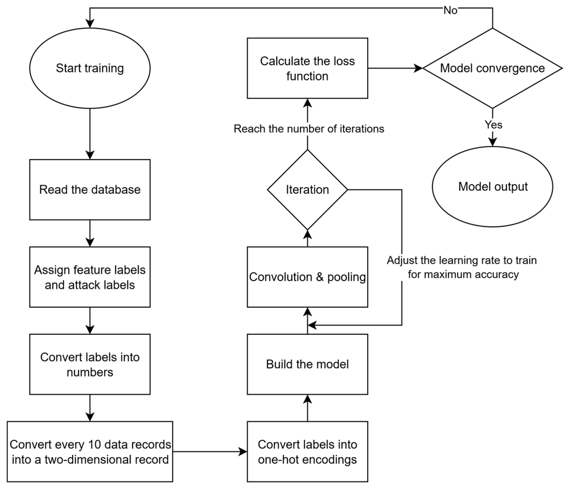
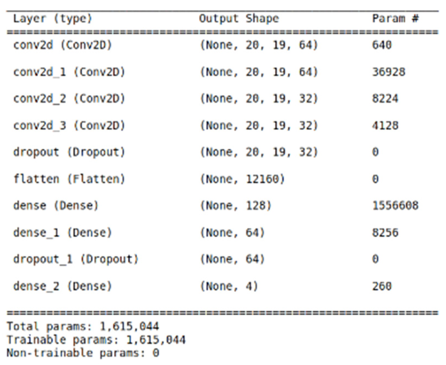
After preprocessing, the data were reshaped into a two-dimensional format in which every 10 consecutive samples form a single input matrix. We use a rolling-window scheme so that the most recent 10 records are fed to the CNN for each prediction. This window length is chosen to capture short-horizon burst patterns commonly observed in attack traffic while avoiding unnecessary buffering. In our ablation across window sizes (3, 5, 10, 20, and 50), accuracy gains beyond 10 were small, whereas the latency and memory overhead increased. In real-time operation, the additional delay is essentially the time to accumulate 10 samples plus one forward pass of the lightweight CNN; under high-rate conditions the window fills quickly, and on-device inference keeps the overall impact on real-time performance minimal. The overall training process is shown in Figure 11, and the network architecture in Figure 12.

3.5.3. Long Short-Term Memory (LSTM)

The LSTM is an improved variant of the Recurrent Neural Network (RNN) and is well-suited for processing and predicting time series data. In this study, the LSTM model was implemented using the Keras framework.
The collected dataset was first labeled, and complex attributes such as timestamps, IP addresses, and MAC addresses were converted into numerical values using the LabelEncoder function from the Scikit-learn (sklearn) library. Subsequently, the OneHotEncoder function was applied to transform each categorical feature into a machine-readable numeric format—effectively digitizing the feature space.
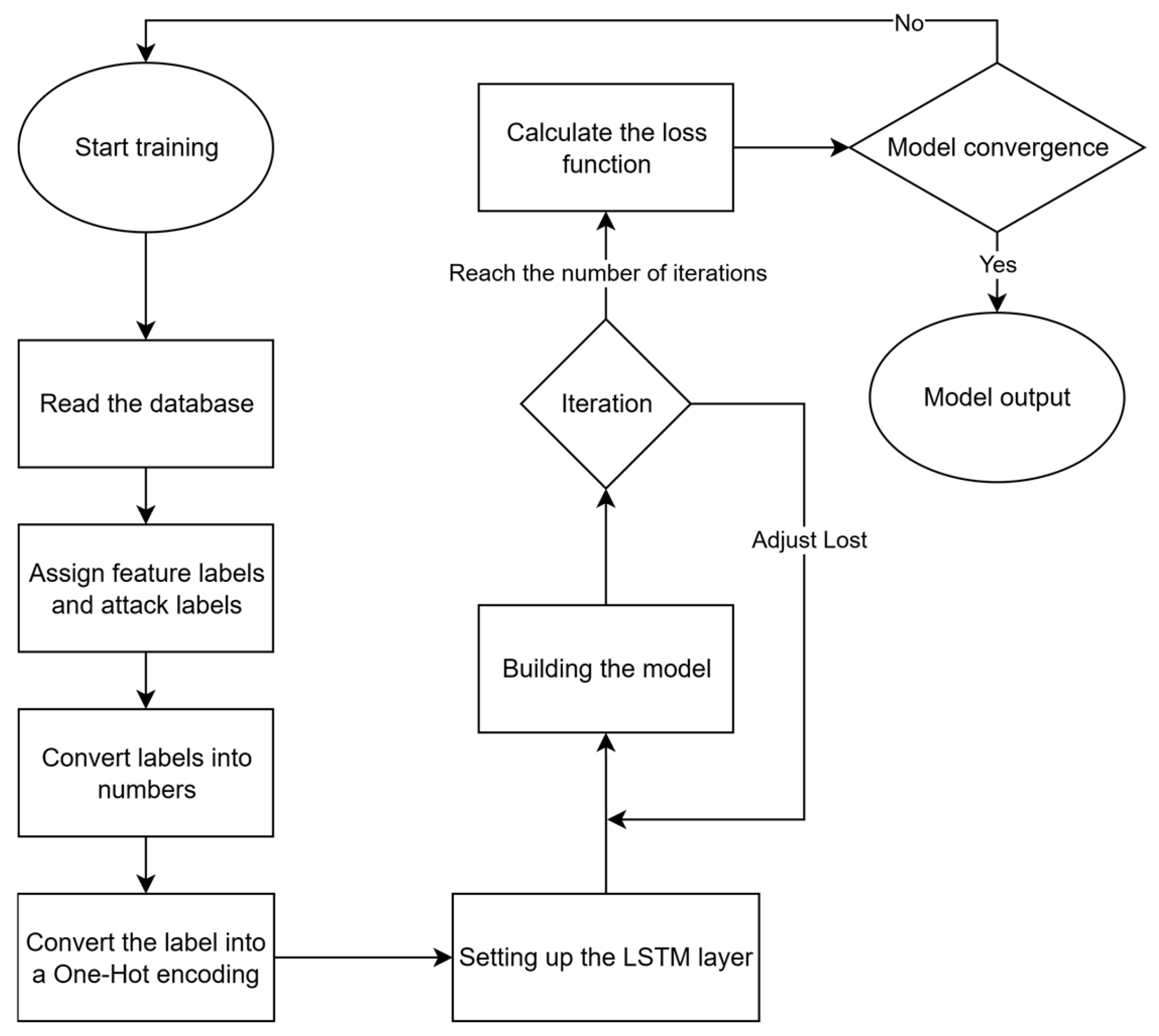
After preprocessing, the input data were structured using a sliding window approach, where every 10 consecutive records were treated as a sequence (timestep) to predict the 11th record. Unlike the CNN model, which treats 10 records as a 2D matrix for convolution, the LSTM model uses the temporal order of the 10 records to learn sequential patterns and predict future behavior. The overall training process is illustrated in Figure 13, and the architecture of the LSTM network is shown in Figure 14.

4. Results

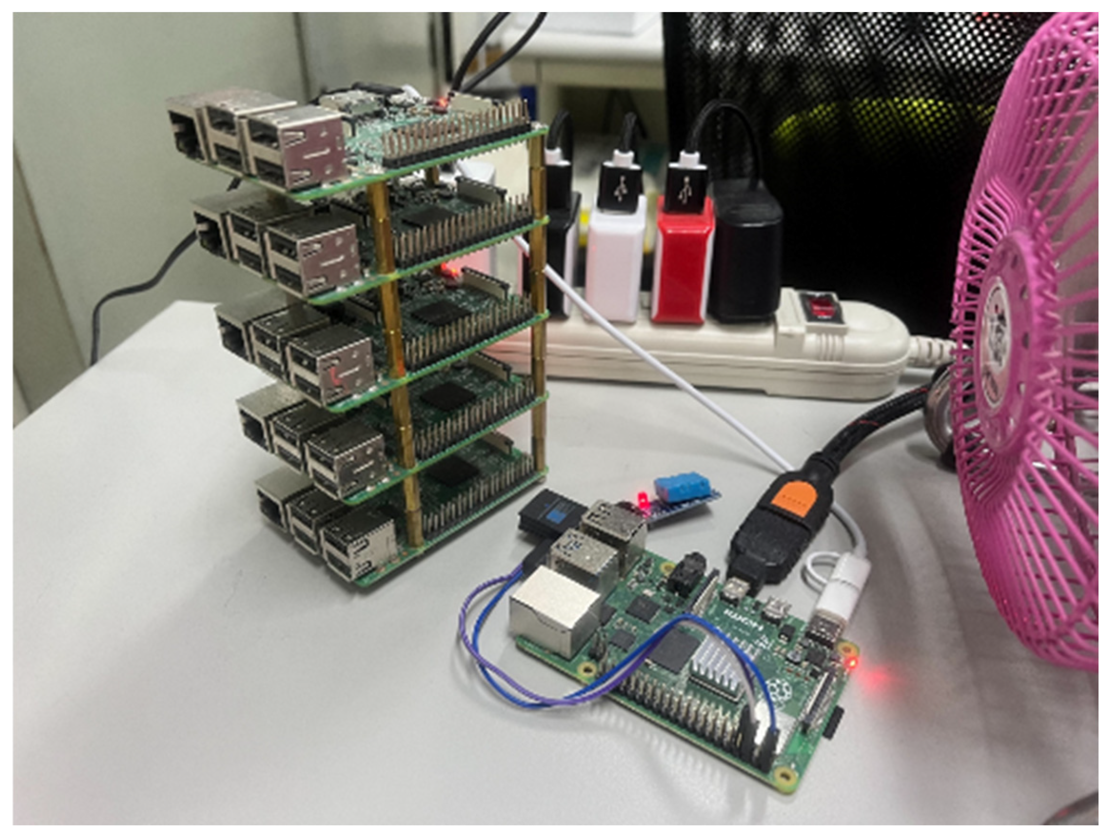
This study is implemented on a oneM2M-based IoT application platform. A Raspberry Pi 4 is used as the sensing node, as shown on the right side of Figure 15, functioning as a micro single-board computer. It corresponds to both the MN-AE (Middle Node–Application Entity) and MN-CSE (Middle Node–Common Services Entity) components in the oneM2M architecture and serves as the data storage device within the field domain. It is hereafter referred to as Pi 4.
Five Raspberry Pi 3 devices, shown on the left side of Figure 15, are used as attack nodes to simulate IoT devices compromised by botnets.
An edge computing computer is deployed as the server representing the infrastructure domain. It receives data from Pi 4 via IP1 and stores them locally. Simultaneously, it captures network packets from IP1 using Tshark (via IP2) for analysis. After completing the classification and detection process, the result is sent back to Pi 4 through a socket connection. Based on the received result, Pi 4 then performs the corresponding defense actions.

4.1. Data Transmission from IoT Sensing Node

A Pi 4 reads temperature and humidity from the sensor using a Python script and sends the readings to Node-RED via an HTTP POST request to the “Post Smart Home Data” node. In Node-RED, a Function node formats the payload as a JSON object, and the JSON is then forwarded to the MN-CSE node. Figure 16 provides a schematic overview of this workflow.
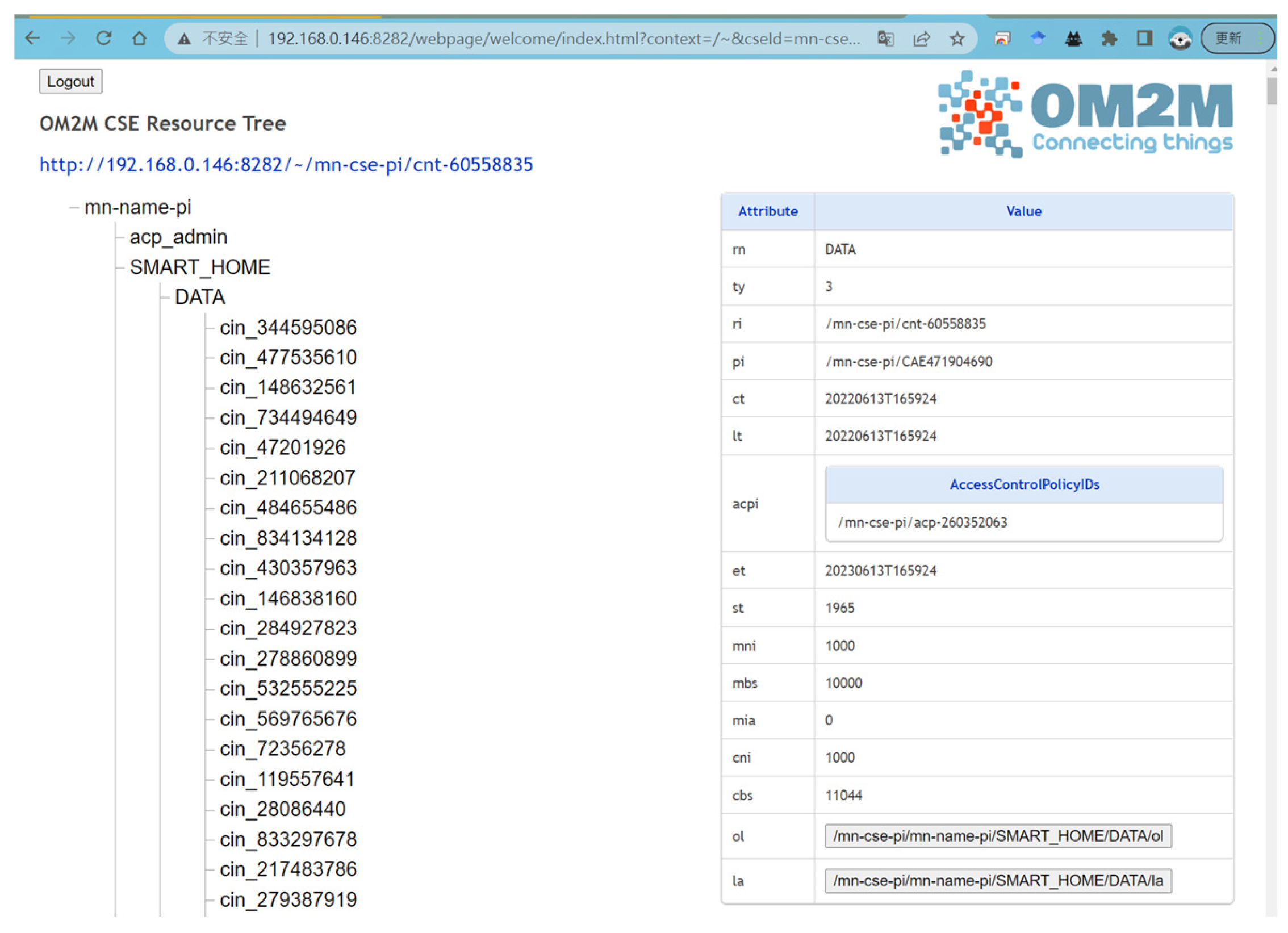
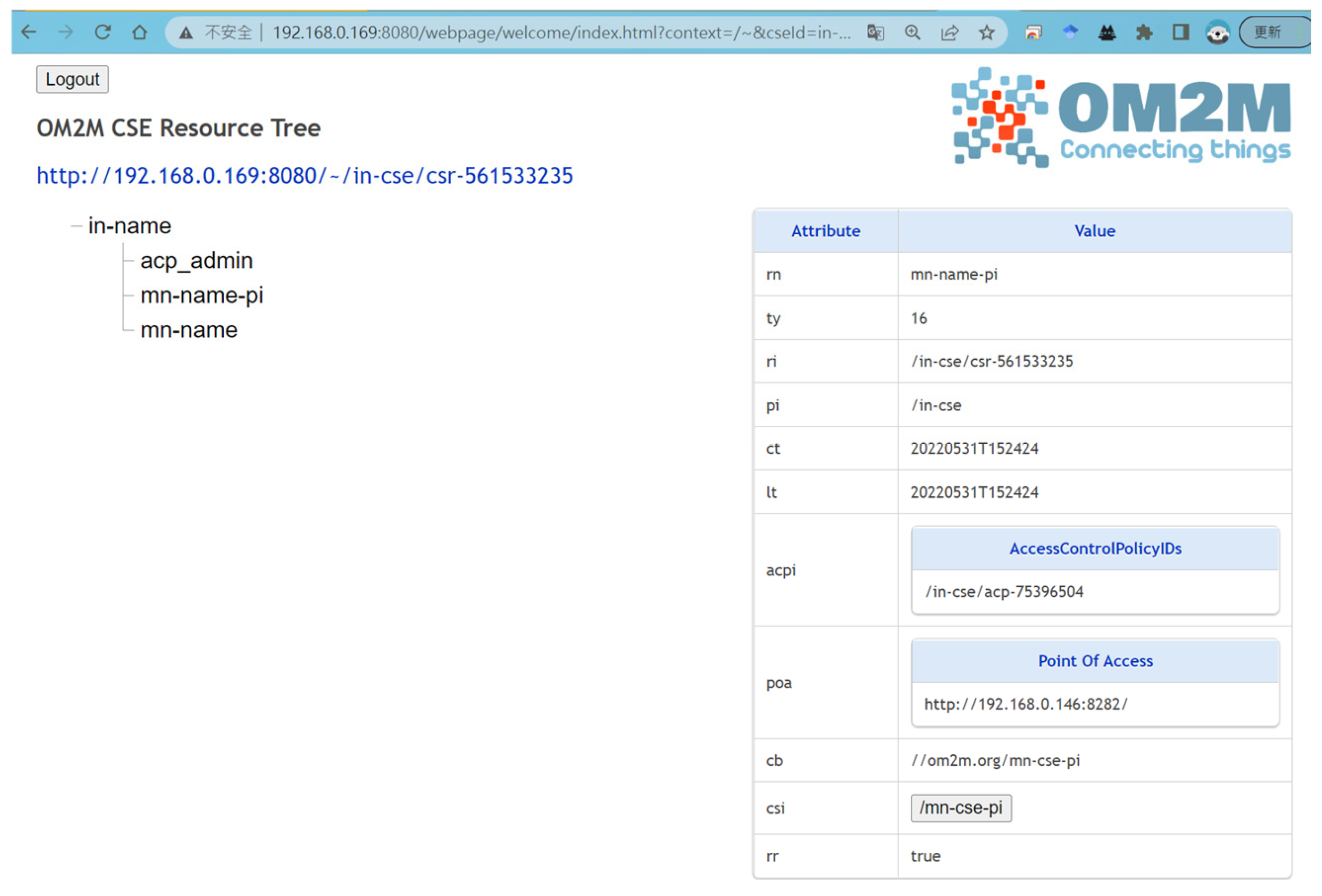
Figure 17 and Figure 18 present the node information for the MN-CSE and IN-CSE, respectively. As shown in Figure 17, the DATA container includes sensor data that were imported from the IN-CSE node illustrated in Figure 18. For example, the data entry labeled cin344595086 represents a single piece of sensor data within the DATA container. This name is randomly generated by the platform.
The IN-CSE node shown in Figure 18 serves as the central management node, capable of managing multiple MN nodes. By clicking the “csi” button corresponding to/mn-cse-pi on the right side of Figure 18, the interface will redirect to the MN-CSE view shown in Figure 17.

4.2. Data Access

Packets captured from IP2 of a Pi 4 device. The dataset contains four different traffic conditions: normal, SYN flood, UDP flood, and ICMP flood. For each condition, 50,000 packets were collected as training and validation datasets.
After training the model using this dataset, an initial accuracy score is obtained. Subsequently, a separate test dataset, collected independently under the same four conditions, is used to evaluate the model again. This second round of testing yields a second accuracy score, which is expected to better reflect real-world performance and ensures that the model is not overfitting the training data.

4.3. DoS Attack Architecture and Its Impact on the Server

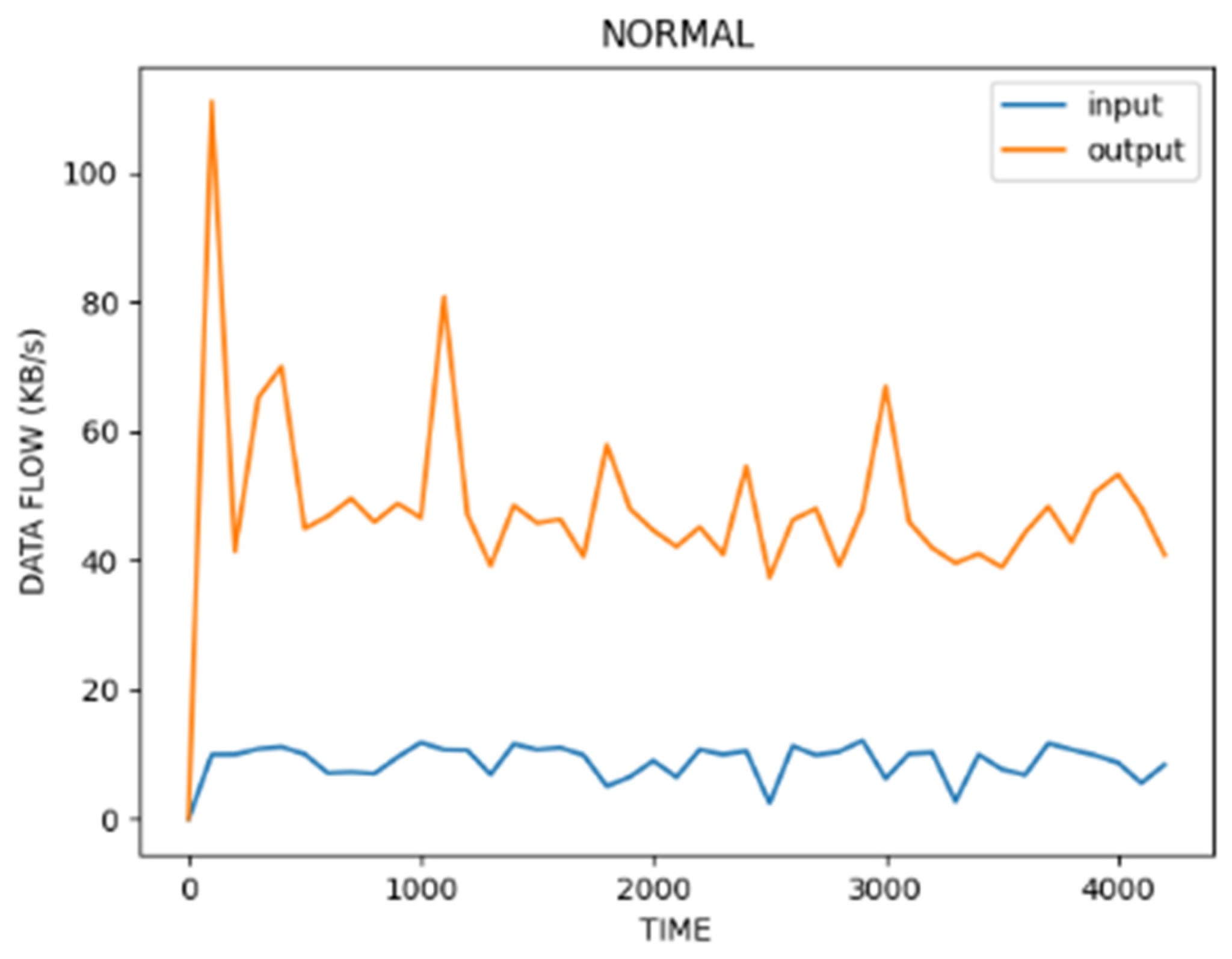
Figure 19 presents CPU and memory utilization together with inbound and outbound network throughput during normal Raspberry Pi 4 operation. The mean inbound rate is approximately 10 kB/s, and the mean outbound rate is approximately 50 kB/s. The data were collected over the same one-minute period as in Figure 20, comprising about 20 records.
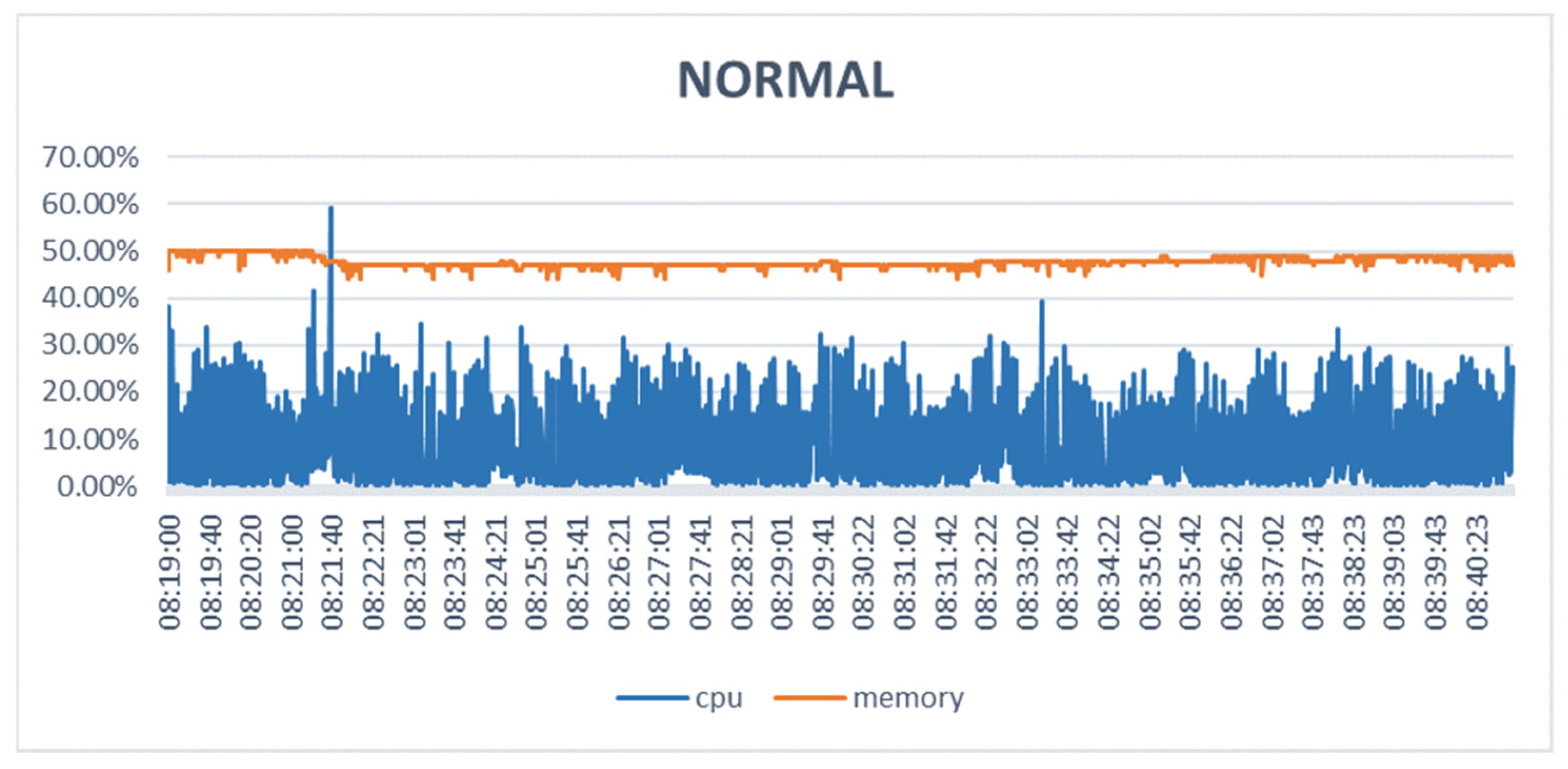
From Figure 20, it can be observed that during the normal transmission of sensor data to the oneM2M platform, memory usage remains stable at around 50%, and CPU usage fluctuates between 20% and 30%.
Figure 21 shows the CPU and memory utilization and the inbound/outbound network traffic of the Raspberry Pi 4 during the SYN flood attack. Inbound traffic averages about 10 kB/s, whereas outbound traffic varies widely, peaking at roughly 400 kB/s. The measurement window matches that of Figure 22, with ~20 samples collected over one minute.
From Figure 22, it can be observed that while sensor data are still being transmitted to the oneM2M platform, memory usage remains around 50%. However, CPU usage exhibits sharp spikes, periodically rising to 20–30% before dropping back to around 5%, resembling a “needle-like” fluctuation pattern under stress.
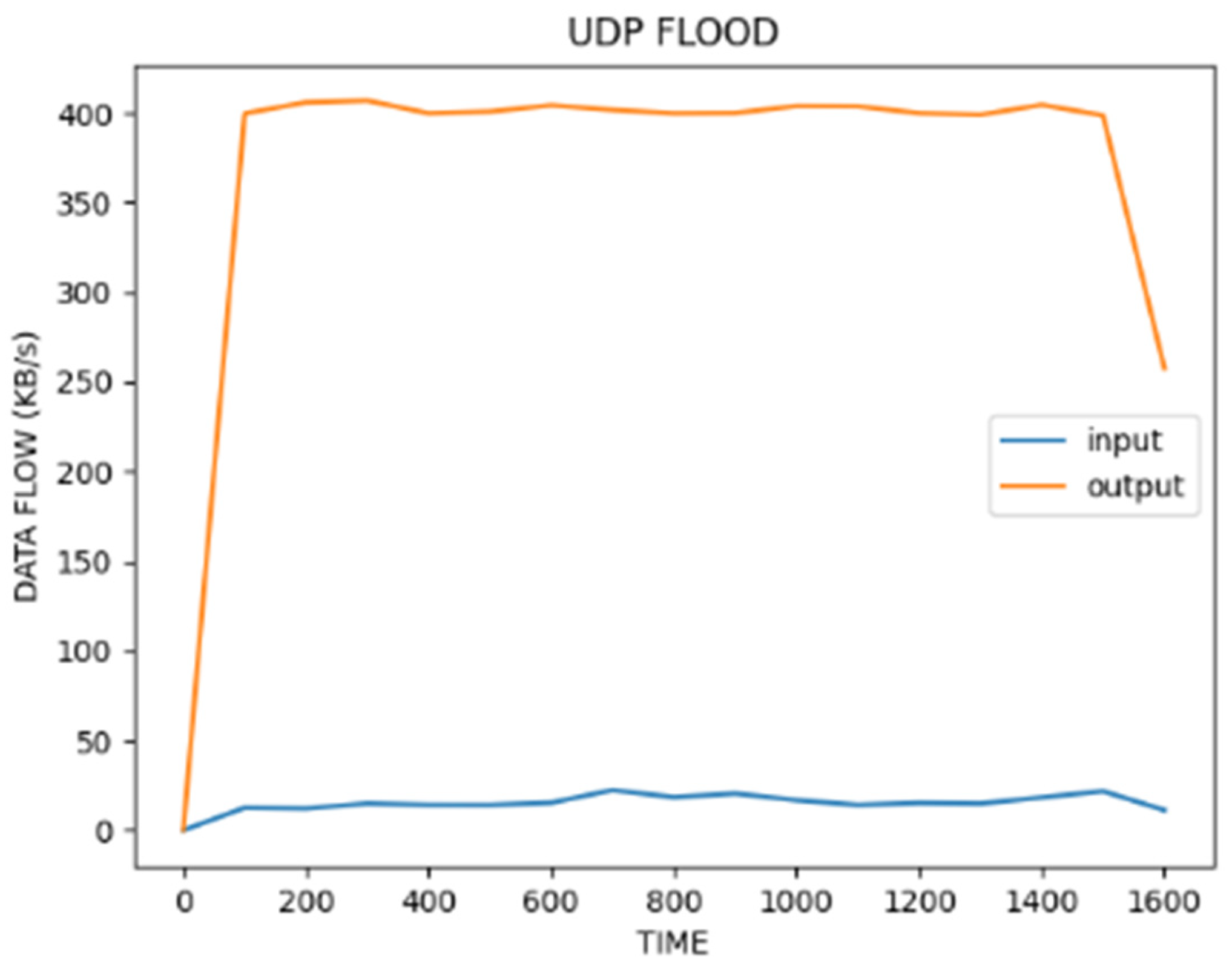
Figure 23 presents CPU and memory utilization together with inbound and outbound network throughput for the Raspberry Pi 4 under a UDP flood attack. The inbound rate remains near 10 kB/s, while the outbound rate is consistently high at approximately 400 kB/s. The data were collected over the same one-minute interval as in Figure 24, comprising about 20 samples.
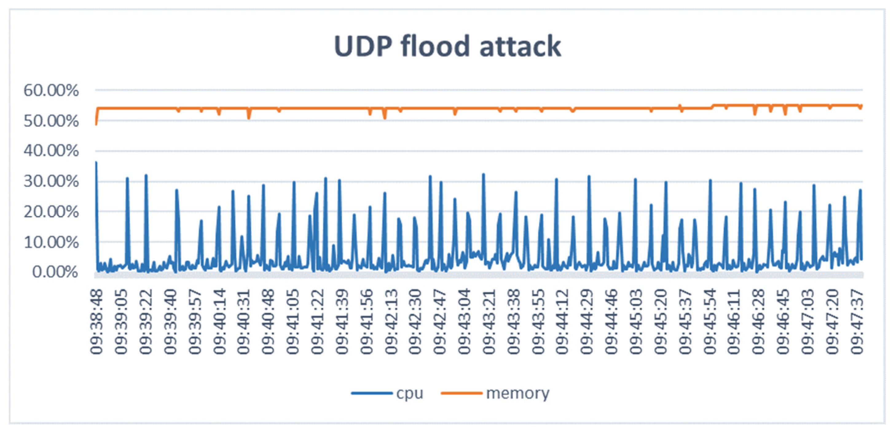
From Figure 24, it can be observed that during sensor data transmission to the oneM2M platform under attack, memory usage remains steady at approximately 50%. However, the CPU usage exhibits frequent spike patterns, similar to the behavior under a SYN flood attack, but with higher spike frequency. CPU usage typically rises to 20–30% and then quickly drops back to around 5%, reflecting the stress imposed by the high volume of incoming UDP packets.
Figure 25 presents CPU and memory utilization together with inbound and outbound network throughput for the Raspberry Pi 4 under an ICMP flood attack. Relative to the other attack scenarios, the inbound rate is substantially higher, reaching approximately 1500 kB/s at its peak; the outbound rate peaks around 400 kB/s. The data were collected over the same one-minute interval as in Figure 26 (20 records).
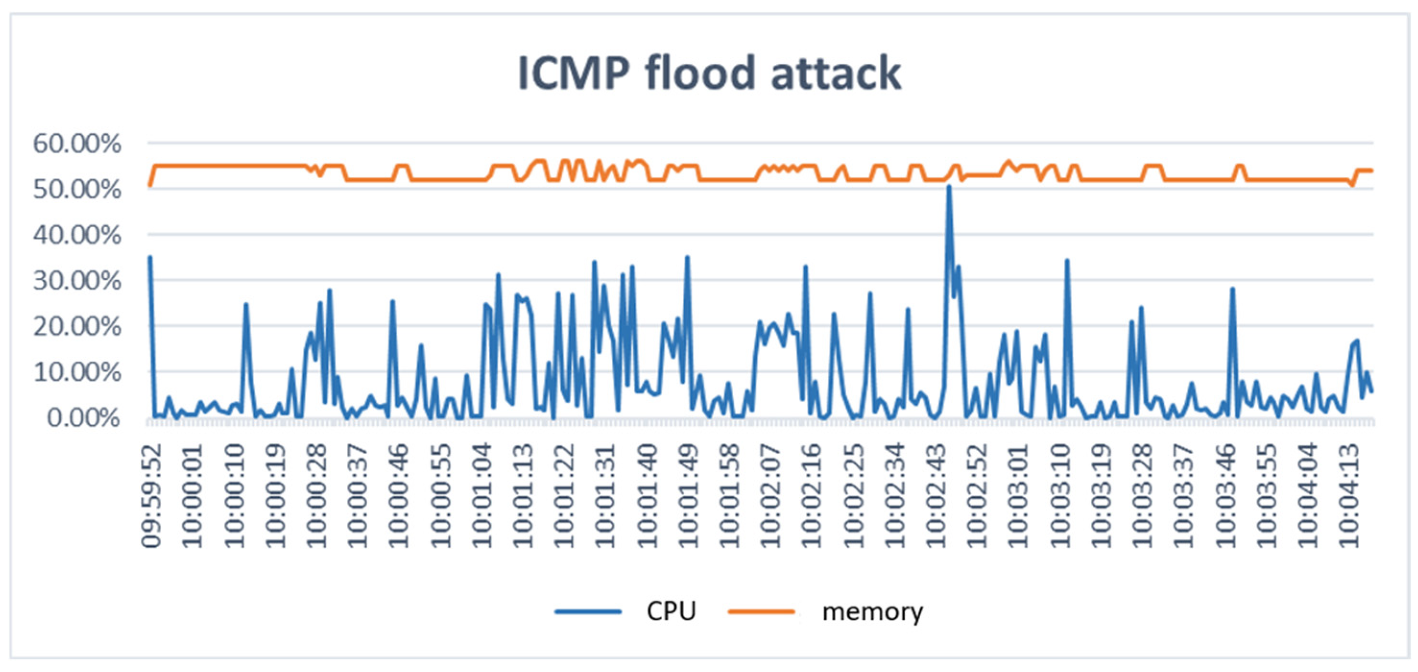
As shown in Figure 26, during sensor data transmission to the oneM2M platform under ICMP flood attack, memory usage remains around 50%, similar to prior conditions. However, CPU usage exhibits a different pattern, with peaks reaching up to 30% and troughs dropping as low as 0%, indicating a fluctuating but heavy load from continuous ICMP processing.

4.4. Edge Computing System and Model Training Process

We also connect results to protocol mechanics by explaining which features drive correct classifications and confusions.
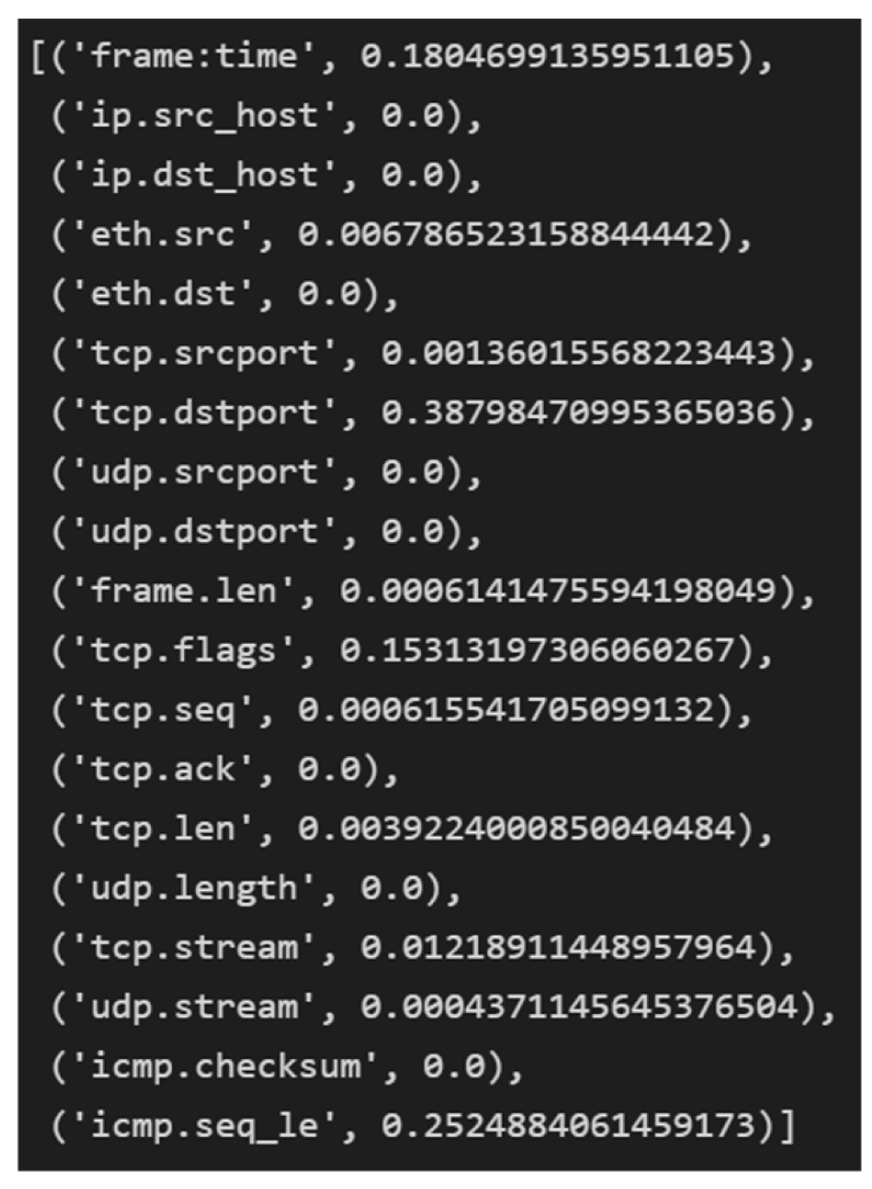
In this section, the constructed dataset is evaluated using varying input sample sizes as labeled training data. Three models—Decision Tree (DT), 2D Convolutional Neural Network (2D-CNN), and LSTM—are trained and compared based on their classification accuracy. The best-performing models are selected for practical testing and deployment. Under SYN floods, elevated tcp.flags SYN without matching ACKs stresses the half-open queue; the model relies most on tcp.flags and tcp.dstport. UDP floods present sustained, connectionless bursts with low entropy in udp.dstport/udp.length. ICMP floods yield dense echo sequences with monotone icmp.seq_le. These protocol-level signatures align with decision-tree feature importance (Figure 27) and explain occasional UDP–ICMP confusions when payload sizes and burst patterns converge.
The accuracy rate is derived from the confusion matrix shown in Table 2 and is calculated using Equation (5).
A c c u r a c y = T P + T N T P + T N + F P + F N × 100 %

4.4.1. Decision Tree Model

In this subsection, the Decision Tree model was trained using individual data records as input, with random_state fixed at 25. Several hyperparameters—including splitter, min_samples_leaf, max_depth, and min_samples_split—were adjusted to determine the optimal configuration for accuracy.
Table 3 presents the accuracy results for the main hyperparameter tuning. The highest accuracy of 94.17% was achieved when max_depth was set to 9. Modifying min_samples_leaf and min_samples_split did not significantly improve model performance.
Table 4 shows the tuning results for min_impurity_decrease. Although a value of 0.0005 achieved the best accuracy on the validation set, it performed poorly on the test set. Therefore, 0.001 was selected as the final value for better generalization.
Table 5 compares the performance of different splitter settings. The random option was chosen over the best due to its superior test accuracy and reduced risk of overfitting. The best option yielded only 41.81% accuracy on the test set, indicating severe overfitting.
Figure 27 shows the feature importance derived from the trained Decision Tree model. The most influential features were frame:time, tcp.dstport, tcp.flags, and icmp.seq_le.

4.4.2. Two-Dimensional Convolutional Neural Network (2D-CNN)

The two-dimensional convolutional neural network (2D-CNN) was trained using input features consisting of 3, 5, and 10 data records, under varying training configurations. Each configuration was trained for 10, 20, and 50 epochs with a batch size of 512 and learning rates set to 0.0001, 0.0005, and 0.001, respectively. The model architecture comprises three convolutional layers with 64, 32, and 32 neurons, respectively. A dropout layer was added after the third convolutional layer to prevent overfitting, followed by a ReLU activation function. A flatten layer was applied to transform the multi-dimensional feature maps into a one-dimensional vector, which was then passed through two fully connected layers. Finally, a Softmax activation function was used in the output layer for classification.
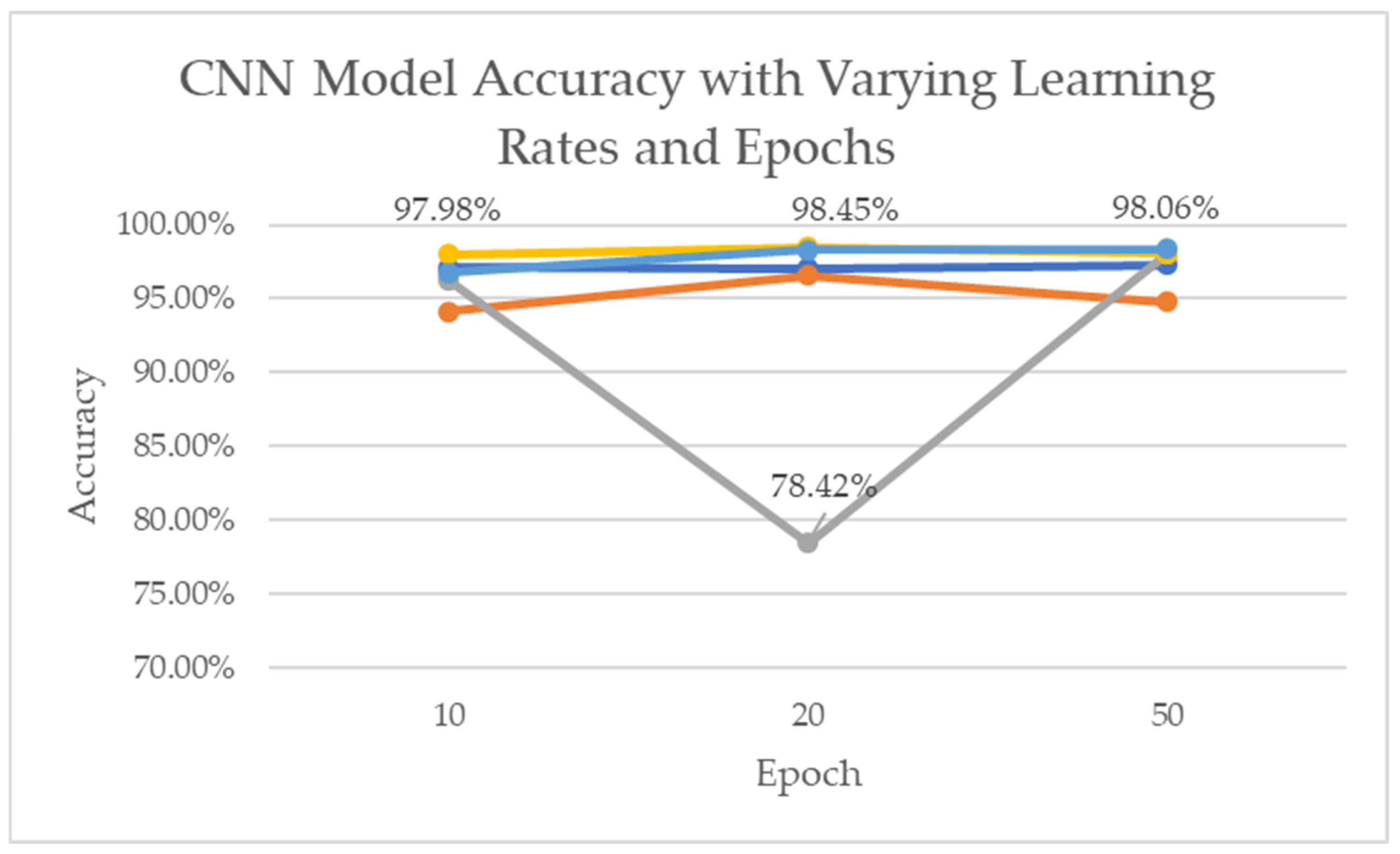
To assess model convergence speed and classification accuracy under different input sizes, various training settings were tested. Results showed that with a learning rate of 0.0001 and 50 epochs, the highest testing accuracy reached 97.29%. When the learning rate was set to 0.0005 and trained for 20 epochs, the best accuracy was 96.58%. With a learning rate of 0.001 and 50 epochs, the highest accuracy achieved was 98.45%. Another setting with a learning rate of 0.0005 and 20 epochs yielded 98.06%, and using 0.0001 for 50 epochs resulted in 98.39%. Based on overall performance, the optimal configuration was determined to use 20 input records, a learning rate of 0.0005, and 20 training epochs. These results were compiled into a summary chart (Figure 28), where different colors represent the number of input records: dark blue for 3, orange for 5, gray for 10, yellow for 20, and light blue for 50.

4.4.3. LSTM Model

The LSTM model was trained using input feature sequences consisting of 3, 5, 10, and 20 records. For each configuration, training was performed for 10, 20, and 50 epochs with a batch size of 512. The model architecture includes two LSTM layers with 64 and 128 units, respectively, each followed by a dropout layer to prevent overfitting. The sigmoid activation function was applied within the LSTM layers. Afterward, a fully connected layer was added, and the output layer employed the Softmax activation function for multi-class classification.
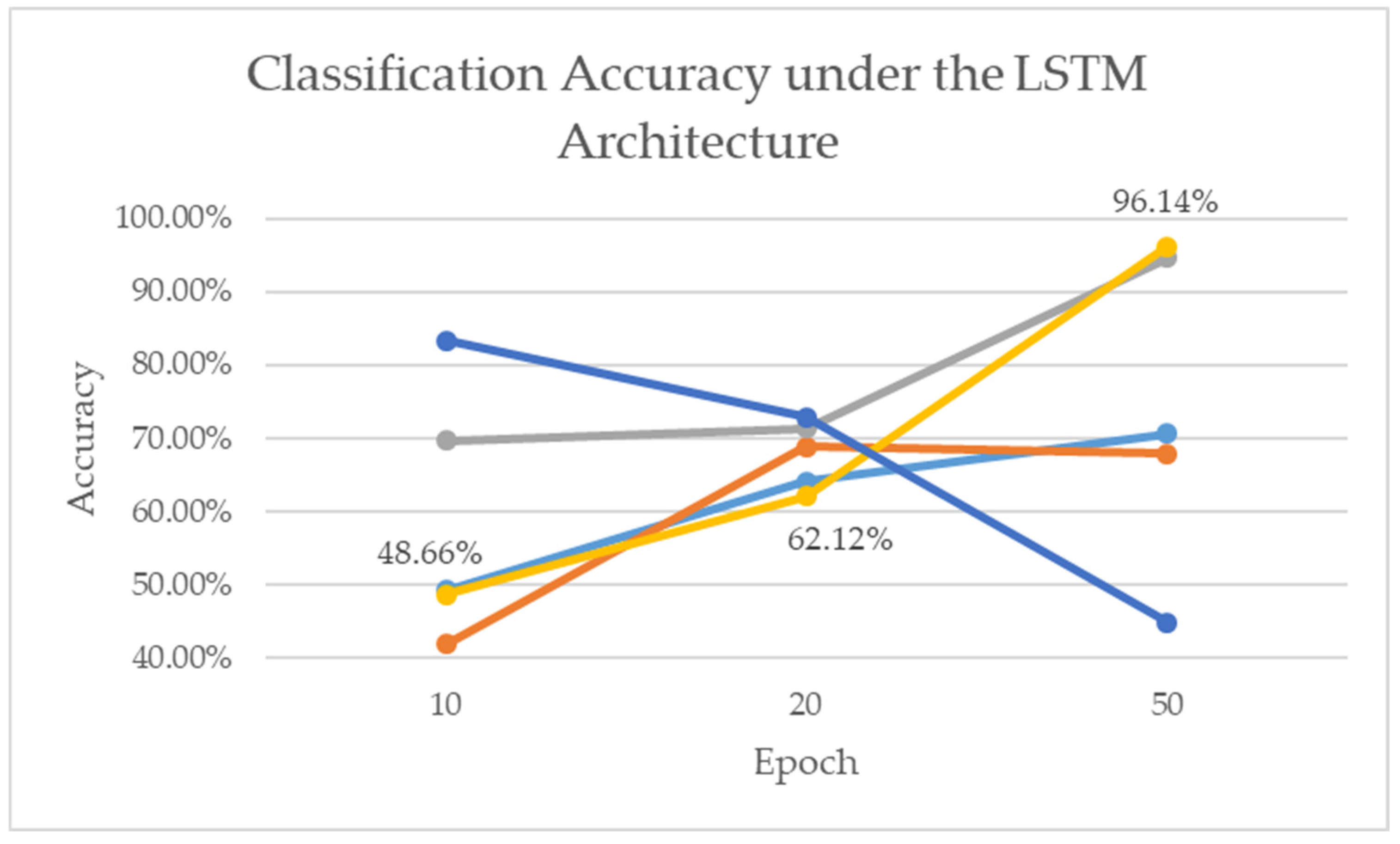
To evaluate how the number of input records affects convergence speed and model accuracy under a fixed architecture, various input lengths and training settings were tested. The results were compiled into a summary chart (Figure 29), where different colors represent different input sizes: dark blue for 3 records, orange for 5 records, gray for 10 records, yellow for 20 records, and light blue for 50 records.

4.5. Practical Application

Based on the above results, the CNN model demonstrated the highest classification accuracy among all models evaluated in this study, achieving an accuracy of 98.45% under the configuration of a 0.0005 learning rate and 20 training epochs. The LSTM model, due to its limited effectiveness with short input sequences, was unable to fully leverage its temporal modeling capabilities and reached a maximum accuracy of only 96.14%. The Decision Tree (DT) model, being relatively simple, performed less accurately compared to CNN and LSTM, with a maximum accuracy of 93.77%. While suitable for basic classification tasks, its performance is likely to degrade significantly as more attack types are introduced.
In this section, the CNN model—identified as the most accurate—will be used for real-world testing. Specifically, the oneM2M server (Pi 4, referred to as IP2) was used to record transmission data under four conditions: normal traffic, SYN flood attacks, UDP flood attacks, and ICMP flood attacks. Feature data extracted from traffic sent by IP1 to IP2 were transmitted via sockets to an edge computing device running the trained CNN model. After processing, the model returned its classification result to Pi 4. If the traffic was identified as normal, only the result was returned; if any attack was detected, the corresponding defense mechanism was triggered.
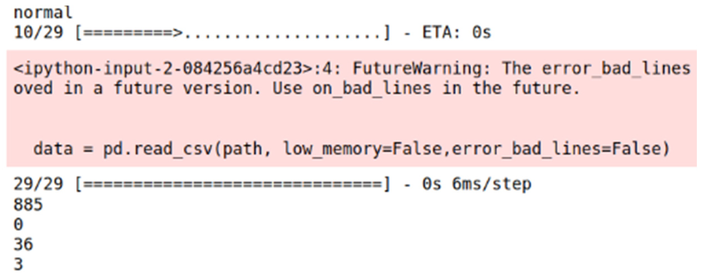
Figure 30 shows the edge computing classification results under normal traffic conditions.
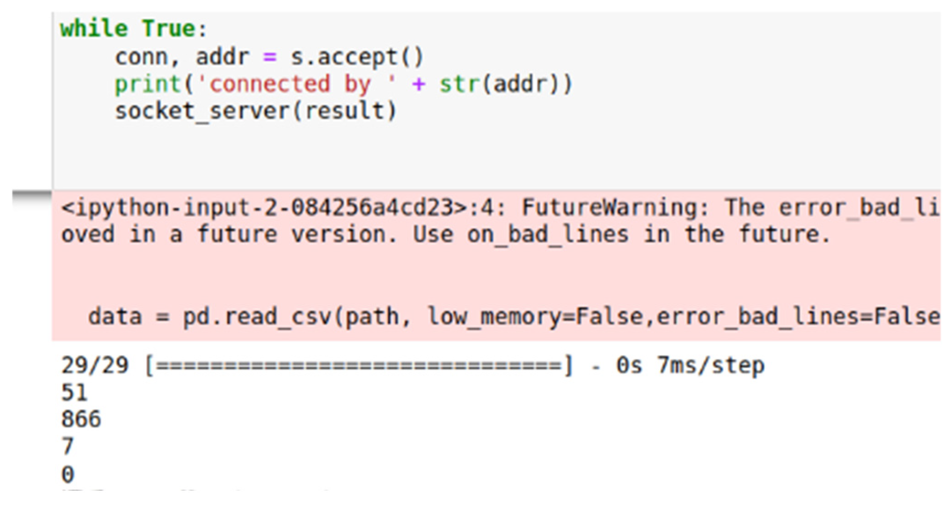
If a SYN flood attack is detected, the Pi 4 device will execute a shell script to enable the SYN cookie mechanism. Under such an attack, the server’s half-open connection queue quickly becomes saturated, causing new connection requests to be dropped. The SYN cookie technique allows the server to continue handling incoming SYN requests even when the half-open connection queue is full.
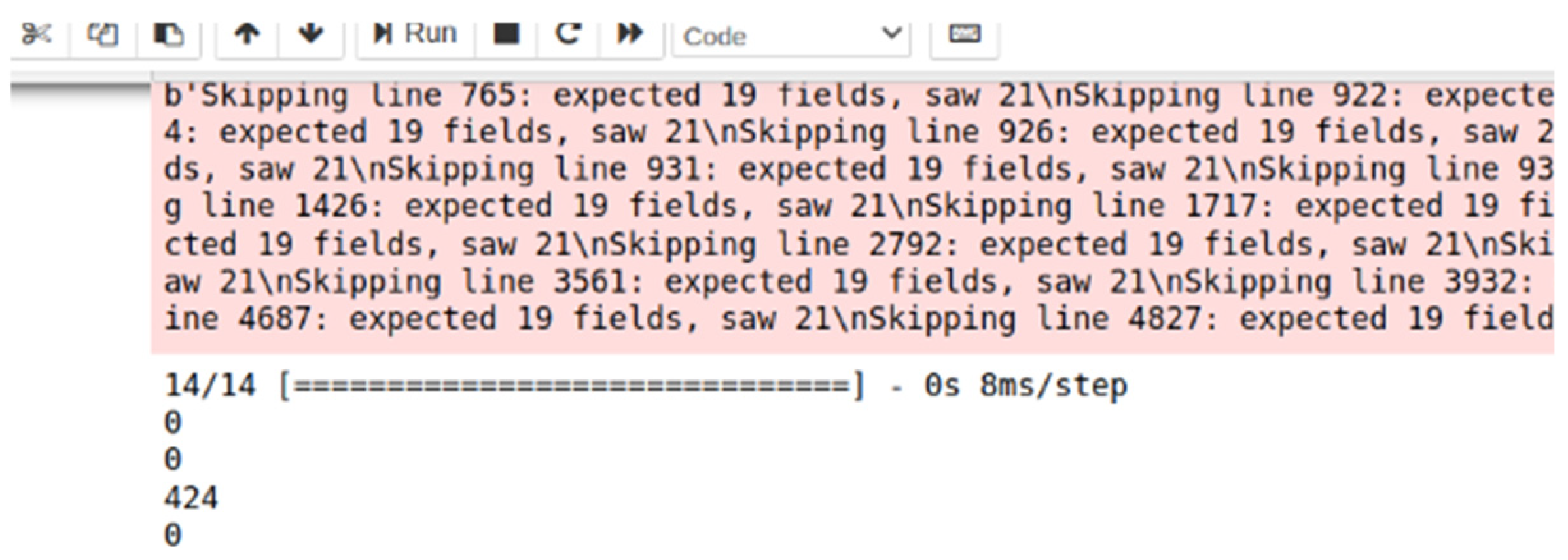
Figure 31 presents the edge computing inference results under a SYN flood scenario.
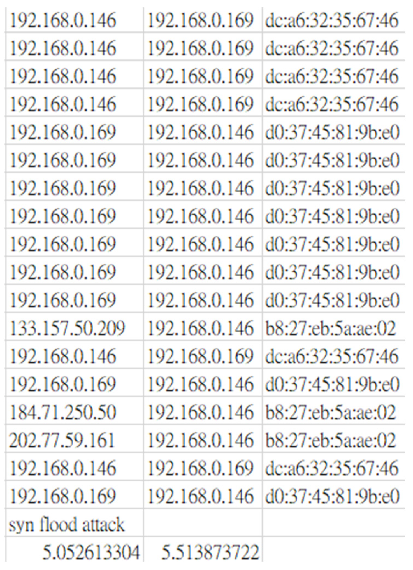
Figure 32 displays the packet capture data after enabling the SYN cookie mechanism. During the SYN flood attack, the first 200 packets were collected within 5.05 s. After enabling SYN cookies, the collection time for 200 packets increased to 5.51 s, indicating that the server was able to continue accepting new SYN requests despite the queue being full.
If a UDP flood attack is detected, the Pi 4 device will execute a shell script to apply UDP-related firewall rules. This action activates the firewall to mitigate the impact of the attack, allowing the device sufficient time to alert the administrator for further intervention.
Figure 33 presents the edge computing inference results under a UDP flood attack.
If an ICMP flood attack is detected, the Pi 4 device will execute a shell script to apply ICMP traffic rate-limiting rules. This is implemented using the iptables firewall to block excessive ICMP packets. Once traffic levels return to normal, the rate-limiting rules are removed.
Figure 34 presents the edge computing results under an ICMP flood attack.

5. Conclusions

This paper aims to detect and defend against DDoS attacks targeting the internal network of an IoT server system based on the oneM2M architecture. To reduce the high cost of additional security hardware for IoT devices, we propose an edge computing-based real-time monitoring and defense system for detecting DDoS attacks on IoT servers. The system transmits network packets from IP1 to an edge computing device through a private IP2 channel. These packets are then analyzed using three classification algorithms—Decision Tree (DT), Convolutional Neural Network (CNN), and LSTM—to identify the type of DDoS attack and apply appropriate countermeasures accordingly. This enables users to respond promptly and mitigate the impact of the attacks.
For defense mechanisms, SYN cookie techniques are employed to counter SYN flood attacks, while UDP flood and ICMP flood attacks are mitigated by configuring iptables firewall rules to block malicious traffic. Experimental results show that the proposed methods successfully defend against SYN flood and ICMP flood attacks. However, under UDP flood attacks, even when all packets are dropped, the system still experiences performance degradation and becomes unresponsive, requiring manual administrator intervention.
The use of machine learning and deep learning models enhances DDoS detection accuracy while simultaneously reducing dependency on specific software and hardware environments. It also simplifies real-time updates and the upgrade process for detection strategies. Future improvements can be explored in the following four directions: (1) expanding the types of attacks covered to increase the generalizability of the models; (2) incorporating hardware-level indicators (e.g., CPU usage and packet rates) into the training dataset to improve detection accuracy—though this may trade off detection speed; (3) integrating public datasets for training or validation to enhance model reliability; and (4) improving defense strategies, as the current methods only partially alleviate attack impacts. More advanced defense mechanisms can be explored to build a more robust and comprehensive system.

Author Contributions

Methodology, Y.-H.C.; validation, C.-H.C.; formal analysis, Y.-Y.L. All authors have read and agreed to the published version of the manuscript.

Funding

This research received no external funding.

Data Availability Statement

Data are contained within this article.

Conflicts of Interest

The authors declare no conflicts of interest.

References

  1. Verma, S.; Kawamoto, Y.; Kato, N. A Network-Aware Internet-Wide Scan for Security Maximization of IPv6-Enabled WLAN IoT Devices. IEEE Internet Things J. 2021, 8, 8411–8422. [Google Scholar] [CrossRef]
  2. Bellini, P.; Nesi, P.; Pantaleo, G. IoT-Enabled Smart Cities: A Review of Concepts, Frameworks and Key Technologies. Appl. Sci. 2022, 12, 1607. [Google Scholar] [CrossRef]
  3. Forsey, C. The 13 Best Smart Home Devices & Systems of 2021. Available online: https://blog.hubspot.com/marketing/smart-home-devices (accessed on 24 February 2021).
  4. Washizaki, H.; Ogata, S.; Hazeyama, A.; Okubo, T.; Fernandez, E.B.; Yoshioka, N. Landscape of Architecture and Design Patterns for IoT Systems. IEEE Internet Things J. 2020, 7, 10091–10101. [Google Scholar] [CrossRef]
  5. Eskandari, M.; Janjua, Z.H.; Vecchio, M.; Antonelli, F. Passban IDS: An Intelligent Anomaly-Based Intrusion Detection System for IoT Edge Devices. IEEE Internet Things J. 2020, 7, 6882–6897. [Google Scholar] [CrossRef]
  6. Tushir, B.; Dalal, Y.; Dezfouli, B.; Liu, Y. A Quantitative Study of DDoS and E-DDoS Attacks on WiFi Smart Home Devices. IEEE Internet Things J. 2020, 8, 6282–6292. [Google Scholar] [CrossRef]
  7. Bock, P. Lessons Learned from a Forensic Analysis of the Ukrainian Power Grid Cyberattack. Available online: https://blog.isa.org/lessons-learned-forensic-analysis-ukrainian-power-grid-cyberattack-malware (accessed on 31 August 2025).
  8. Arifin, M.A.S.; Stiawan, D.; Suprapto, B.Y.; Susanto, T.; Salim, T.; Idris, M.Y.; Shenify, M.; Budiarto, R. A Novel Dataset for Experimentation with Intrusion Detection Systems in SCADA Networks Using IEC 60870-5-104 Standard. IEEE Access 2024, 12, 170553–170569. [Google Scholar] [CrossRef]
  9. Abou El Houda, Z.; Khoukhi, L.; Senhaji Hafid, A. Bringing Intelligence to Software Defined Networks: Mitigating DDoS Attacks. IEEE Trans. Netw. Serv. Manag. 2020, 17, 2523–2535. [Google Scholar] [CrossRef]
  10. Odumuyiwa, V.; Alabi, R. DDoS Detection on Internet of Things Using Unsupervised Algorithms. J. Cyber Secur. Mobil. 2021, 10, 569–592. [Google Scholar] [CrossRef]
  11. Sangodoyin, A.O.; Akinsolu, M.O.; Pillai, P.; Grout, V. Detection and Classification of DDoS Flooding Attacks on Software-Defined Networks: A Case Study for the Application of Machine Learning. IEEE Access 2021, 9, 122495–122508. [Google Scholar] [CrossRef]
  12. Ferrag, M.A.; Friha, O.; Hamouda, D.; Maglaras, L.; Janicke, H. Edge-IIoTset: A New Comprehensive Realistic Cyber Security Dataset of IoT and IIoT Applications for Centralized and Federated Learning. IEEE Access 2022, 10, 40281–40306. [Google Scholar] [CrossRef]
  13. Mienye, I.D.; Jere, N. A Survey of Decision Trees: Concepts, Algorithms, and Applications. IEEE Access 2024, 12, 86716–86727. [Google Scholar] [CrossRef]
  14. Huang, Y.-S.; Jiang, J.-H.R. Circuit Learning: From Decision Trees to Decision Graphs. IEEE Trans. Comput.-Aided Des. Integr. Circuits Syst. 2023, 42, 3985–3996. [Google Scholar] [CrossRef]
  15. Lee, J.; Sim, M.K.; Hong, J.-S. Assessing Decision Tree Stability: A Comprehensive Method for Generating a Stable Decision Tree. IEEE Access 2024, 12, 90061–90072. [Google Scholar] [CrossRef]
  16. Li, H.; Song, J.; Xue, M.; Zhang, H.; Song, M. A Survey of Neural Trees: Co-Evolving Neural Networks and Decision Trees. IEEE Trans. Neural Netw. Learn. Syst. 2025, 36, 11718–11737. [Google Scholar] [CrossRef] [PubMed]
  17. Zheng, J.; Gao, Q.; Ogorzałek, M.; Lü, J.; Deng, Y. A Quantum Spatial Graph Convolutional Neural Network Model on Quantum Circuits. IEEE Trans. Neural Netw. Learn. Syst. 2025, 36, 5706–5720. [Google Scholar] [CrossRef]
  18. Li, Z.; Liu, F.; Yang, W.; Peng, S.; Zhou, J. A Survey of Convolutional Neural Networks: Analysis, Applications, and Prospects. IEEE Trans. Neural Netw. Learn. Syst. 2022, 33, 6999–7018. [Google Scholar] [CrossRef] [PubMed]
  19. Anthoniraj, S.; Karthikeyan, P.; Vivek, V. Weed Detection Model Using the Generative Adversarial Network and Deep Convolutional Neural Network. J. Mob. Multimed. 2021, 18, 275–292. [Google Scholar] [CrossRef]
  20. Ma, R.; Wang, Q.; Bu, X.; Chen, X. Real-Time Detection of DDoS Attacks Based on Random Forest in SDN. Appl. Sci. 2023, 13, 7872. [Google Scholar] [CrossRef]
  21. Aldaej, A.; Ahanger, T.A.; Ullah, I. Deep Learning-Inspired IoT-IDS Mechanism for Edge Computing Environments. Sensors 2023, 23, 9869. [Google Scholar] [CrossRef] [PubMed]
  22. Chaira, M.; Belhenniche, A.; Chertovskih, R. Enhancing DDoS Attacks Mitigation Using Machine Learning and Blockchain-Based Mobile Edge Computing in IoT. Computation 2025, 13, 158. [Google Scholar] [CrossRef]
  23. Huang, S.-Y.; An, W.-J.; Zhang, D.-S.; Zhou, N.-R. Image Classification and Adversarial Robustness Analysis Based on Hybrid Quantum–Classical Convolutional Neural Network. Opt. Commun. 2023, 533, 129287. [Google Scholar] [CrossRef]
  24. Ding, Y.; Li, Z.; Zhou, N. Quantum Generative Adversarial Network Based on the Quantum Born Machine. Adv. Eng. Inform. 2025, 68, 103622. [Google Scholar] [CrossRef]
  25. oneM2M. Available online: https://www.onem2m.org/ (accessed on 31 August 2025).
  26. Babita; Kaushal, S.; Kumar, H. Interworking of M2M and oneM2M. In Proceedings of the 2022 International Conference for Advancement in Technology (ICONAT), Goa, India, 21–22 January 2022; pp. 1–4. [Google Scholar] [CrossRef]
  27. Saini, P.; Mahajan, N.; Kaushal, S.; Kumar, H. An analytical survey on optimized authentication techniques in OneM2M. In Proceedings of the 2023 International Conference on Innovative Data Communication Technologies and Application (ICIDCA), Uttarakhand, India; 2023; pp. 721–729. [Google Scholar] [CrossRef]
  28. Gupta, R.; Naware, V.; Vattem, A.; Hussain, A.M. A Wi-SUN network-based electric vehicle charging station using Open Charge Point Protocol (OCPP) and oneM2M platform. In Proceedings of the 2024 IEEE Applied Sensing Conference (APSCON), Goa, India; 2024; pp. 1–4. [Google Scholar] [CrossRef]
  29. oneM2M. TS-0001: Functional Architecture; oneM2M: Nice, France, 2019. [Google Scholar]
  30. Fielding, R.T. Architectural Styles and the Design of Network-Based Software Architectures. Ph.D. Thesis, University of California, Irvine, CA, USA, 2000. [Google Scholar]
  31. Wazzan, M.; Algazzawi, D.; Bamasaq, O.; Albeshri, A.; Cheng, L. Internet of Things botnet detection approaches: Analysis and recommendations for future research. Appl. Sci. 2021, 11, 5713. [Google Scholar] [CrossRef]
  32. Singh, M.; Singh, M.; Kaur, S. Issues and challenges in DNS-based botnet detection: A survey. Comput. Secur. 2019, 86, 28–52. [Google Scholar] [CrossRef]
  33. Wallarm Cybersecurity Center. UDP Flood Attack. Available online: https://www.wallarm.com/what/udp-flood-attack (accessed on 31 August 2025).
  34. zaheernew. The Overview of ICMP—PART 03. Available online: https://forum.huawei.com/enterprise/en/the-overview-of-icmp-part-03/thread/807857-867?page=2 (accessed on 31 August 2025).
  35. Khan, A.; Fouda, M.M.; Do, D.-T.; Almaleh, A.; Rahman, A.U. Short-term traffic prediction using deep learning long short-term memory: Taxonomy, applications, challenges, and future trends. IEEE Access 2023, 11, 94371–94388. [Google Scholar] [CrossRef]
  36. Martin, B.; Gilmore, C.; Jeffrey, I. A long short-term memory approach to incorporating multifrequency data into deep-learning-based microwave imaging. IEEE Trans. Antennas Propag. 2024, 72, 7184–7196. [Google Scholar] [CrossRef]
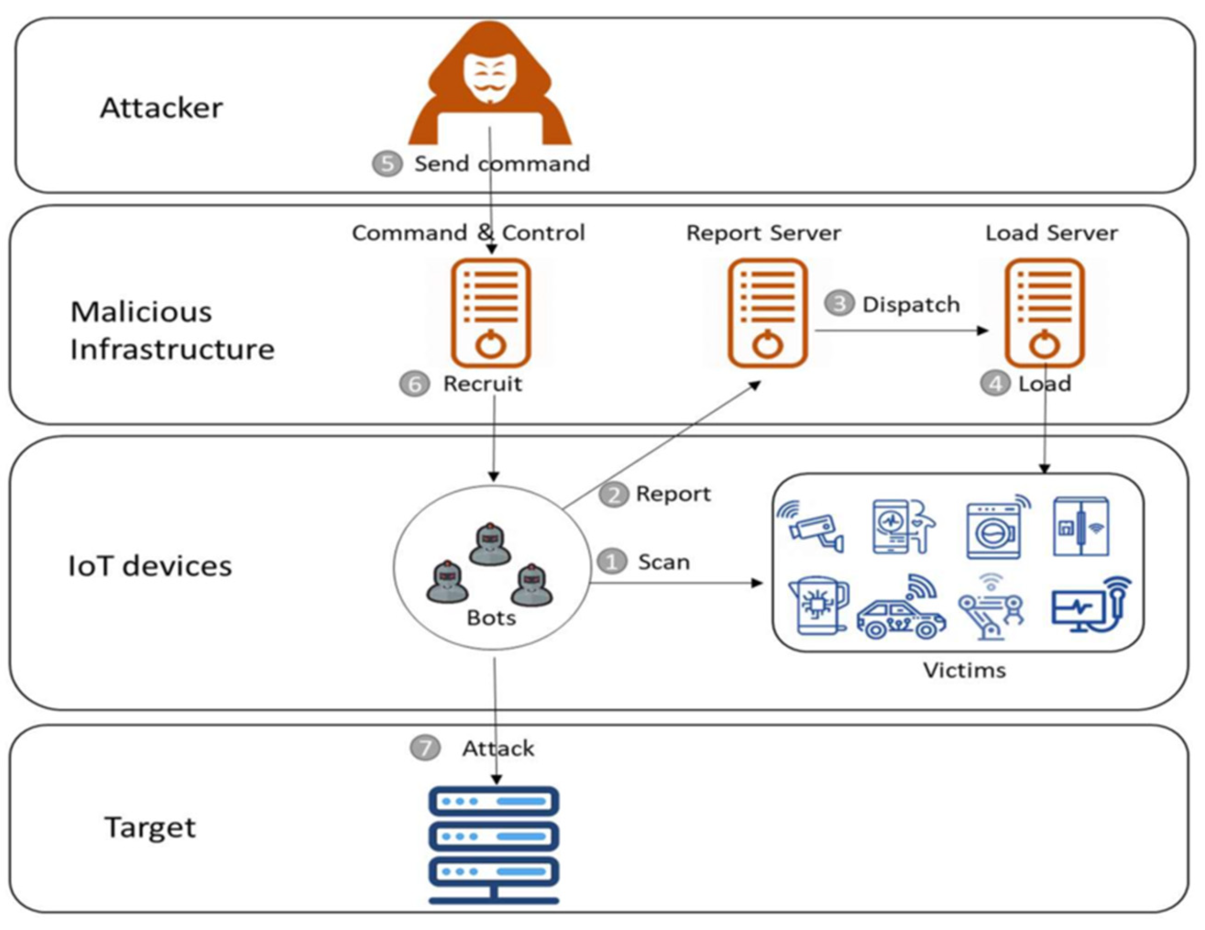
Figure 1. IoT botnet process flow.
Futureinternet 17 00411 g001
Figure 2. Simple-RNN diagram.
Futureinternet 17 00411 g002
Figure 3. LSTM simple structure diagram.
Futureinternet 17 00411 g003
Figure 4. Training model and attack identification and prevention flow chart.
Futureinternet 17 00411 g004
Figure 5. Raspberry Pi 3 (left) and Raspberry Pi 4 (right).
Futureinternet 17 00411 g005
Figure 6. Smart home based on oneM2M architecture.
Futureinternet 17 00411 g006
Figure 7. Edge computing transmission flowchart.
Futureinternet 17 00411 g007
Figure 8. Architecture diagram for collecting packet signatures.
Futureinternet 17 00411 g008
Figure 9. Commands used in this experiment.
Futureinternet 17 00411 g009
Figure 10. Decision Tree model training process.
Futureinternet 17 00411 g010
Figure 11. CNN Model Training Process.
Futureinternet 17 00411 g011
Figure 12. Network architecture of the CNN model.
Futureinternet 17 00411 g012
Figure 13. LSTM model training process.
Futureinternet 17 00411 g013
Figure 14. Network architecture of the LSTM model.
Futureinternet 17 00411 g014
Figure 15. IoT sensing node and attack devices.
Futureinternet 17 00411 g015
Figure 16. Schematic of the Data Transmission Process.
Futureinternet 17 00411 g016
Figure 17. Configuration details of the MN-CSE node.
Futureinternet 17 00411 g017
Figure 18. Configuration details of the IN-CSE node.
Futureinternet 17 00411 g018
Figure 19. Network ingress and egress traffic under normal conditions.
Futureinternet 17 00411 g019
Figure 20. CPU and memory utilization under normal conditions.
Futureinternet 17 00411 g020
Figure 21. Incoming and outgoing network traffic during a SYN flood attack.
Futureinternet 17 00411 g021
Figure 22. CPU and memory usage under SYN flood attack.
Futureinternet 17 00411 g022
Figure 23. Inbound and outbound network traffic during a UDP flood attack.
Futureinternet 17 00411 g023
Figure 24. CPU and memory status during a UDP flood attack.
Futureinternet 17 00411 g024
Figure 25. Inbound and outbound network traffic during an ICMP flood attack.
Futureinternet 17 00411 g025
Figure 26. CPU and memory status during an ICMP flood attack.
Futureinternet 17 00411 g026
Figure 27. Feature importance of the Decision Tree.
Futureinternet 17 00411 g027
Figure 28. CNN model accuracy with varying learning rates and epochs.
Futureinternet 17 00411 g028
Figure 29. Classification accuracy under the LSTM architecture.
Futureinternet 17 00411 g029
Figure 30. Edge computing results under normal conditions.
Futureinternet 17 00411 g030
Figure 31. Edge computing results under SYN flood attack.
Futureinternet 17 00411 g031
Figure 32. Packet data after SYN cookie are enabled.
Futureinternet 17 00411 g032
Figure 33. Edge computing results under UDP flood attack.
Futureinternet 17 00411 g033
Figure 34. Edge computing results under ICMP flood attack.
Futureinternet 17 00411 g034
Table 1. Dataset parameters.
NoNameProtocolTypeDescription
1frame.timeFrameDate and timeThe timestamp when the packet was received.
2ip.src_hostIPCharacter stringThe IP address of the source host.
3ip.dst_hostIPCharacter stringThe IP address of the destination host.
4eth.srcMACCharacter stringThe MAC address of the sending device.
5eth.dstMACCharacter stringThe MAC address of the receiving device.
6tcp.srcportTCPUnsigned integerThe source port number for the TCP packet.
7tcp.dstportTCPUnsigned integerThe destination port number for the TCP packet.
8udp.srcportUDPUnsigned integerThe source port number for the UDP packet.
9udp.dstportUDPUnsigned integerThe destination port number for the UDP packet.
10frame.lenFrameUnsigned integerThe total length of the packet in bytes.
11tcp.flagsTCPLabelControl flags used in the TCP header.
12tcp.seqTCPUnsigned integerThe sequence number assigned to the TCP segment.
13tcp.ackTCPUnsigned integerThe acknowledgment number indicates the next expected byte.
14tcp.lenTCPUnsigned integerThe size of the TCP header.
15udp.lengthUDPUnsigned integerThe total length of the UDP packet.
16tcp.streamTCPUnsigned integerThe stream identifier for the TCP connection.
17udp.streamUDPUnsigned integerThe stream identifier for the UDP connection.
18icmp.checksumICMPUnsigned integerThe checksum value is used for error detection.
19icmp.seq_leICMPUnsigned integerThe sequence number in ICMP echo requests or replies.
20Attack_label/NumberBinary label: 0 for normal traffic and 1 for attack traffic.
21Attack_type/Character stringThe specific type of attack (e.g., SYN flood, UDP flood, and ICMP flood).
Table 2. Confusion matrix.
PredictNormal Transmission Is PredictedPredicted to Be Under Attack
Predict
Normal TransmissionTP (correct judgment, normal transmission)FN (error judgment, normal transmission)
Under AttackFP (false positive judgment, abnormal transmission)TN (correct judgment, abnormal transmission)
Table 3. Accuracy achieved after tuning decision tree hyperparameters.
Parameter Value12345678910
Parameter Type
max_depth48.71%87.45%88.36%92.42%93.27%92.42%93.92%93.71%94.17%93.86%
min_samples_leafXXXX94.17%94.17%94.17%94.17%94.17%94.17%
min_samples_splitX94.17%94.17%94.17%94.17%94.17%94.17%94.17%94.17%94.17%
Table 4. Accuracy achieved after tuning the min_impurity_decrease parameter.
Parameter Value0.10.010.0050.0010.0005
Min_Impurity_Decrease
Validation set accuracy87.45%88.33%93.51%94.17%94.22%
Test set accuracy88.47%89.32%93.76%93.77%45.71%
Table 5. Accuracy achieved after tuning the splitter parameter.
SplitterRandomBest
Result
Validation set accuracy94.17%97.53%
Test set accuracy93.77%41.81%
Disclaimer/Publisher’s Note: The statements, opinions and data contained in all publications are solely those of the individual author(s) and contributor(s) and not of MDPI and/or the editor(s). MDPI and/or the editor(s) disclaim responsibility for any injury to people or property resulting from any ideas, methods, instructions or products referred to in the content.