Parallel Agent-Based Framework for Analyzing Urban Agricultural Supply Chains

Abstract

This work presents a parallel agent-based framework designed to analyze the dynamics of vegetable trade within a metropolitan area. The system integrates agent-based and discrete event techniques to capture the complex interactions among farmers, vendors, and consumers in urban agricultural supply chains. Decision-making processes are modeled in detail: farmers select crops based on market trends and environmental risks, while vendors and consumers adapt their purchasing behavior according to seasonality, prices, and availability. To efficiently handle the computational demands of large-scale scenarios, we adopt an optimistic approximate parallel execution strategy. Furthermore, we introduce a credit-based load balancing mechanism that mitigates the effects of heterogeneous communication patterns and improves scalability. This framework enables detailed analysis of food distribution systems in urban contexts, offering insights relevant to smart cities and digital agriculture initiatives.

1. Introduction

Computer simulation is a powerful tool widely used to model, analyze, and evaluate dynamic aspects of a system at different scales of complexity and precision. There are two highly effective yet fundamentally distinct approaches: agent-based modeling and discrete event simulations (DESs). DESs, along with their respective models, describe real-world systems that are complex to model analytically, in which changes in system variables occur in a discrete manner [1]. They have been widely used to gain insight into linear and process-driven systems. Agent-based modeling (ABM) provides a framework that enables the exploration of systems with interactive, adaptive, diverse, and in some cases spatially explicit intelligent decision makers [2]. It is effective in capturing the complex interactions among autonomous entities within a system.

Hybrid approaches [3,4,5,6] that integrate DES and ABM capabilities mark a significant advancement in the field of computational simulation. These models leverage the strengths of both approaches but often demand more complex implementation designs and particular attention to the integration points between them.

In this work, we present a framework that combines both ABS and DES approaches to model the supply chain of fruits and vegetables. In particular, we evaluate our proposal using data from two different regions of Chile, the metropolitan city of Santiago and the O’Higgins Region (the sixth region of Chile). Our model includes farmers, fairground workers (FWs) or vendors, and customers. Farmers determine which crops to sow and harvest based on external factors such as market prices, while yields can be impacted by conditions like frost, drought, and pests. FWs decide which products to purchase from farmers based on seasonality, pricing, and other factors. Meanwhile, customers make purchasing decisions based on their budgets and household size.

The simulation of this complex case study requires the management of multiple agents and a large number of events related to product purchases and agent interactions. Consequently, these simulations demand significant execution time. To address this challenge, we present an approximate optimistic parallel [7] implementation of our simulator. The logical processors (LPs) of the model are distributed among the processors using the Simulated Annealing (SA) [8] metaheuristic. Our approach incorporates a load-balancing algorithm designed to minimize the impact of heterogeneous communication patterns and workload distribution. The algorithm uses the concept of credit, meaning that when an FW initially purchases a product from a farmer (both hosted by different processors), it is assumed that the purchase will be successful. If so, the credit is canceled. Otherwise, if the farmer does not have enough of the requested product, the FW incurs a debt with both the product and the farmer, which will be canceled once the original requested quantity is replenished. Therefore, the contributions of this paper are as follows:

• A hybrid ABM-DES simulator to model the supply chain of fruits and vegetables.
• We parallelize the hybrid ABM-DES simulation using an approximate optimistic approach and the SA metaheuristic to partition the model among the processors.
• We present a load-balance algorithm based on credits to reduce communication among processors.

The remainder of this paper is organized as follows. In Section 2, we present related work. In Section 3, we present the production and sales dynamics in the supply chain of fruits and vegetables as our case study. Section 4 presents the proposed simulation model. Section 5 presents the parallel design of our simulator and the proposed load-balance algorithm. Section 6 presents the experimental results. Section 8 concludes the paper.

2. Related Work

This section provides a comprehensive review of recent studies and methodologies related to simulating farmers’ decision-making processes and agricultural systems. The works discussed here explore various approaches, including agent-based modeling, to understand and predict the behavior of farmers under different scenarios. These studies highlight the complexities of agricultural systems, incorporating factors such as environmental conditions, market dynamics, technological adoption, and policy impacts.

The work in [9] presents a simulation of the decision-making dynamics of small farmers under various scenarios. The input data and models are primarily based on studies and the realities of Czech agriculture. However, the definition of small farmers used in this work shares similarities with ours, including seasonal dependence, a reliance on family labor, and a focus on fruit and vegetable production over livestock. In [9], farmers’ decision-making is influenced by two main factors: the business model and the dynamics of the system in which they operate. On one hand, the business model serves as an analytical strategic tool that defines how a company creates and captures value [10]. According to the authors, this theoretical framework enables the explicit modeling of farmers’ adaptation processes to changes and external factors. The methodology is based on [11] and requires well-specified models, both causally and mathematically. However, this study does not account for the full production flow of small farmers. Specifically, the market with intermediaries and the consumer-driven demand remain implicit as exogenous variables. Additionally, the methodology is predominantly quantitative, meaning certain aspects of agents’ decision-making are not considered. For instance, environmental variables such as climate factors (e.g., frosts, droughts, and heatwaves) are not integrated into the decision-making model.

The study in [12] presents a simulation-based decision support system for small farmers, focusing on a case study in Sri Lanka. In this initiative, the government provides farmers with simulation tools. However, a key implementation challenge arises: the target farmers are largely illiterate. To address this, the proposed system enables users to visually manipulate simulation scenarios, minimizing the need for written interfaces. The methodology is based on mathematical programming [13], a widely used approach in agricultural modeling and analysis, although real-world applications remain limited [14]. The study introduces two mathematical models.

The first model employs a linear formulation, but its main limitation is the inability to represent nonlinear effects, such as the impact of planting a specific crop on adjacent land or across different time periods. To overcome these constraints, the second formulation is designed as a constrained quadratic problem. While this model captures certain nonlinear interactions, it requires relaxing some constraints from the linear formulation, such as individual budget constraints for each farmer. The study does not provide conclusions regarding the accuracy of the simulations.

The study in [15] employed an agent-based model (ABM) to simulate future crop patterns in Luxembourg, incorporating environmental awareness into farmers’ decision-making. The results, used for a life cycle assessment (LCA), reveal that focusing solely on reducing greenhouse gas emissions leads to suboptimal trade-offs. LCA is a methodology used to evaluate the environmental impact of a product, material, or crop throughout its life cycle [16]. The study also compares the bottom-up approach of ABM with a top-down method, highlighting the respective advantages and limitations of each. This work is further expanded in [17]. While the authors acknowledge the importance of using geographically explicit farm data, the simulations were conducted with synthetic polygons representing farms. This work applies social network analysis to study human interactions, where agent relationships are modeled as graphs. Additionally, the authors incorporated a Bayesian model to estimate farmers’ risk aversion throughout the simulation. The model was trained using survey data specifically collected for the project. Although the use of LCA is relatively uncommon in the reviewed literature, the study does not consider risk factors such as frosts, droughts, or pests, nor does it extend the analysis beyond the farmers themselves.

The work in [18] presents a scalable and dynamic agent-based model with environmental boundaries. Unlike other studies, the main actors are not farmers but firms. In this study, the agents do not attempt to optimize a utility function but instead adapt their decision routines, considering social and spatial proximities between agents. The lands are modeled as grids, where farmers can decide to cultivate, deforest, or abandon areas. Firms accumulate the products generated by farmers, which are then traded in the market. However, consumers are not modeled as agents. At each simulation step, the continuity of each firm is evaluated based on its profits at the end of the period. Only theoretical cases were considered.

The work in [19] presents an agent-based modeling framework to predict farmer behavior. The study examines the reactions and behaviors of farmers to changes in climatic factors due to global warming. Different decision functions for farmers were evaluated, such as economic, social, or mixed. The authors conclude that the economic function was the least aligned with the expected outcome. Sixty-eight farms and 23 farmers along the eastern Mediterranean coast were considered as a case study. A simulation horizon of 15 years was used, with annual time steps.

The work in [20] presents a literature review on the modeling of decision-making processes of European farmers. In particular, they focus on agent-based models (ABMs). In this context, an agent is considered any entity capable of perceiving its environment through sensors and acting in response to this perception [21]. Under this scheme, each system is modeled as a set of autonomous entities that perceive, make decisions, and interact with the environment and other entities.

According to [20], ABMs have grown in popularity in the last years. The MP-MAS framework [22] uses dynamic models of interaction and decision-making with dynamic environmental models, particularly with water flow and changes in soil fertility. However, it does not consider environmental risk factors.

The work in [23] proposes a spatial ABM for the evaluation of agricultural policies in relation to the diffusion of innovations and changes in resource use. The simulation is based on empirical data collected in Chile and other regions. In this particular case, the study is conducted in the context of the Mercosur treaty. Almost a decade later, Berger et al. [24] used MP-MAS to study a reservoir project in Ancoa. This project aimed to build a reservoir to store water during the winter period and distribute it during the summer months. This would allow for better planning of the region’s water resources.

The same software is used to study human–environment interaction using ABMs. Tests with data collected in Chile and other regions are presented to study the impact of agricultural policies and the introduction of technologies. However, the MP-MAS and its associated models are not suitable for simulating scenarios where agents make collective decisions [25].

The work in [26] presents an environmental and economic assessment model that utilizes an agent-based approach combined with life cycle thinking methods to simulate bioenergy derived from crop residues. The authors identify farming income, age, farm size, and crop types as the primary factors affecting the adoption of this bioenergy.

The work in [27] aims to evaluate the level of vulnerability of the strawberry agricultural system in Mexico. It presents an agent-based model used to evaluate the vulnerability of the agricultural system through a dynamic analysis of agricultural risk. The authors conclude that temperature and precipitation are key factors influencing strawberry quality.

The work in [28] explores the development and simulation of self-assembling vertical farms for urban agriculture using autonomous systems. It assesses feasibility, structural stability, energy efficiency, and crop optimization to ensure sustainability. By leveraging autonomous technologies, it aims to advance resilient and efficient urban farming.

A recent survey regarding agent-based simulations for agricultural systems can be found in [29].

3. Production and Sales Dynamics in the Supply Chain of Fruits and Vegetables

We model the production and sales chain of fruits and vegetables among smallholder farmers within the metropolitan city of Santiago and in the sixth region of Chile. We aim to study the interactions between farmers, fairground workers, and consumers, and how these interactions are reflected in trade between these actors.

In Chile, the Institute for Agricultural Development (INDAP) (https://www.indap.gob.cl/ (accessed on 11 July 2025)) identifies Family Farming (FF) as small-scale producers, typically residing on the land they cultivate, whose primary source of income is their agricultural activity [30]. This type of production accounts for 54% of the vegetables consumed daily at the national level. Farmers have various channels through which to market their products, with open-air markets being the most popular but offering the least added value. Additionally, FFs are characterized by their low rate of technological adoption compared to other larger entities in the industry. These factors, among others, lead to economic inefficiencies for these small-scale farmers. Therefore, it is important to study the decision-making processes and interaction dynamics among the agents in the production and sales chain.

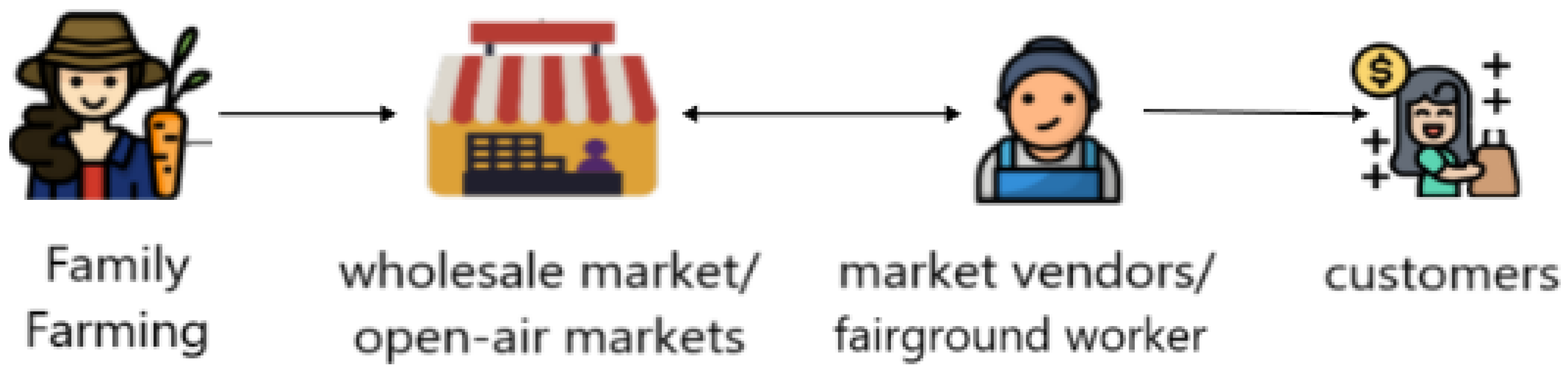
In this work, we evaluate FFs operating within the metropolitan city of Santiago and in the sixth region of Chile. These farmers make decisions about which products to cultivate and when to sell. These decisions are influenced by factors such as the potential profit for a given product and the risk associated with a product based on various climatic variables, such as the probability of heatwaves, droughts, and frosts. The main distributors of the production obtained by the farmers are the market vendors or fairground workers. These agents act as intermediaries between farmers and consumers. They interact with farmers only in a wholesale market, where the supply and demand for large quantities of products takes place (see Figure 1). Additionally, fairground workers sell the acquired products in various open-air markets. These open-air markets are the primary source from which Chilean families obtain fruits and vegetables, and they constitute the main channel for small farmers to reach consumers. An open-air market is understood as a commerce that operates during fixed hours and in specific locations determined by the local government, where products are traded directly with the public—often informally. There are approximately 1114 open-air markets in Chile, with more than 340,000 registered fairground workers [31]. Open-air markets operate at different times and locations, so the prices at which products are sold are not regulated and depend on the territorial characteristics of the market as well as other factors (e.g., climatic conditions).

We consider only fruits and vegetables with a cultivation period of less than one year. This is mainly to observe the decision-making process within a shorter time horizon, as the cultivation of, for example, fruit trees is a high-cost strategic decision that takes years to yield results.

Table 1. Products used in our simulator, with their respective sowing months, commercialization months, and days required to cultivate.

Product	Sowing Months	Selling Months	Days Cult.
Garlic	Apr.–Aug.	All	180
Artichoke	Jan.–Feb.	May–Nov.	90
Celery	All	All	70
Green Pea	May–Aug.	All	90
Broccoli	All	All	90
Corn	Sep.–Dec.	All	120
Cauliflower	All	All	130
Spinach	All	All	90
Broad Bean	Apr.–Jun.	Jan.–May-Dec.	90
Lettuce	All	All	90
Melon	Jan.–Feb.–Sep.–Dec.	Jan.– Mar.–Dec.	120
Salad Cucumber	Sep.–Dec.	All	120
Cranberry Bean	Jan.–Oct.–Dec.	Jan.–May–Dec.	80
Green Bean	Jan.–Sep.–Dec.	All	80
Cabbage	All	All	100
Watermelon	Jan.–Feb.–Sep.–Dec.	Jan.–Mar.–Dec.	120
Tomato	Aug.–Sep.	All	90
Carrot	All	All	120
Zucchini	Jan.–Sep.–Dec.	All	100
Strawberry	Apr.–May	Jan.–May–Oct.–Dec.	120

shows the fruits and vegetables used in our simulator. We show their sowing months, commercialization periods, and average cultivation time in days. Although certain products are cultivated only during specific months of the year, they are available for sale throughout the year due to product imports from other regions.

4. Agent-Based Framework for Analyzing Urban Agricultural Supply Chains

Our simulator includes the entire marketing process of the farmer–fairground workers–consumer chain. The purpose of our simulator is to model the commercialization process of the typical farmer–fairground workers–consumer chain. We aim to analyze the behavior of each participant and the environmental conditions faced by producers during the planting and selling of fruits and vegetables.

The model includes agents representing people such as farmers, fairground workers (FWs) or vendors, and customers. The geospatial space is divided into regions of the city. We assume that each land has a single farmer, and each customer agent buys the products required by its family, aiming to simulate the consumption of the entire population without increasing the number of agents.

The flow of tasks executed by our simulator is detailed in Figure 2. We use event-driven simulation, which allows for greater granularity in specific events, enabling the planning process to interweave events from different processes. The tasks detailed in Figure 2 include:

• Sowing: A farmer—whose land is in an empty state—decides on the product to plant and begins sowing. To this end, the farmer perceives his/her land as empty before starting the crop. The decision about which product to sow involves considering internal elements of the agent (such as whether they have agricultural insurance) and other environmental factors, including the risk of planting a certain product, weather conditions, and price. Farmer agents also perceive environmental and pest risk.
• Harvest: The farmer harvests the product. This process increases the stock of the product based on the size of their land and the efficiency of the product (some products may lose a certain percentage of the production). Then, the farmer restarts the sowing process and starts planning the sale.
• Sale to Wholesale Market: Once the farmer has the inventory of the products, the sale process begins. The wholesale market is an interaction point between agents; it does not store the product. During this process, the farmer informs the market about the products available. That is, the products are stored in an index data structure. Additionally, once the product perishes, it is removed from the index.
• Purchase between fairground workers and farmers: This process takes place in the wholesale market. The fairground workers buy the products during a limited period of time. The fairground workers buy the number of products they estimate they will sell during the day.
• Purchase between fairground workers and customers: Customers go to the wholesale market or to the open-air fairs to buy products from the fairground workers. The wholesale market is open every day, while the open-air fairs are open only one day a week, in different locations. E.g., a given open-air fair located in Providencia, Chile, only opens on Sundays. That is, there are different open-air fairs located in different places, and each one opens on a different weekday.

Figure 2. Fruit and vegetable marketing chain.

Figure 2. Fruit and vegetable marketing chain.

The simulation inputs include Json files and databases. The Json files contain spatial data with information about the locations and the schedule of open-air fairs. It also includes information about the size and location of the agricultural land, along with its boundaries. The database includes information such as the probability of drought, heatwaves, and precipitation, as well as information on products and prices.

Once the simulation begins, we set the initial values for all the variables and the agents:

• Variable initialization: The variables are loaded into the Environment object. This includes climatic variables (probabilities of heat waves, frost, precipitation levels, prices) as well as information related to the products, lands, and fairs.
• Agent initialization: We create the agents—farmers, consumers, and fairground workers. We link the farmers with their corresponding lands. We also link the fairground workers and the consumers with their corresponding open-air fairs.

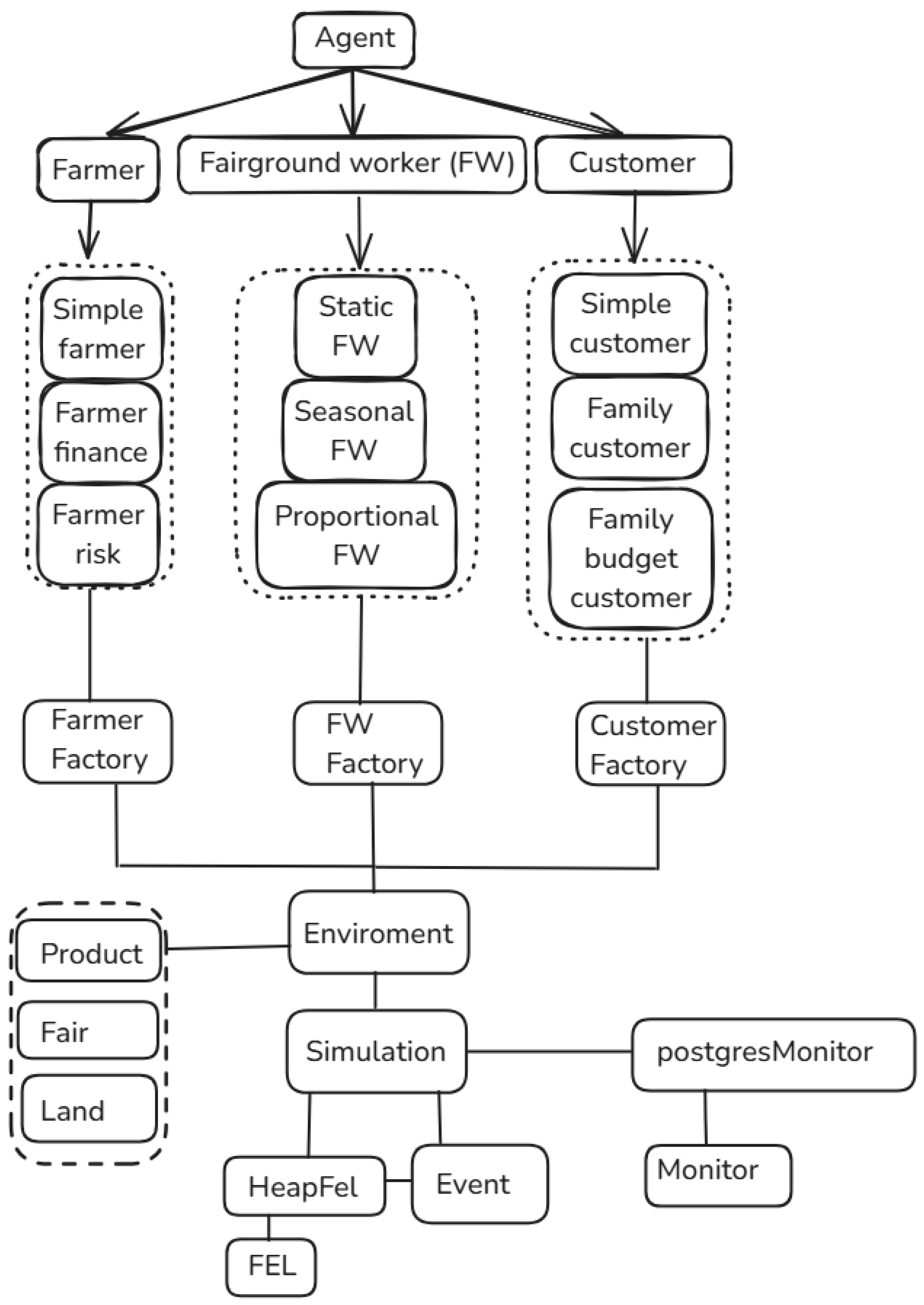
Figure 3 shows the main classes of our simulator. The Simulation class initializes the Environment class, reads parameters and configurations from Json files. It also manages the execution of events and routes them to the corresponding agents. The Environment class manages the instances of the entities (fairs, products, and land) and agents (consumers, fairground workers, and farmers). In addition, it manages the life cycle of the fairs and is responsible for making information available to the entities and agents during the simulation. The Agent class is an abstract class that is the basis for all the types of implemented agents. The Farmer, Fairground Worker (FW), and Consumer classes—rectangles with dotted lines—are abstract classes that define the general life cycle of each agent. For each type of agent, we provide different implementations that can be used for simulation. The Simple Farmer class chooses a random product to grow from those available each month. The Farmer Finance class uses the cost model (expected profit and cost per square meter multiplied by the land size) to determine the product that gives the highest profit when choosing a crop. The Farmer Risk class follows the risk model described in the following section.

The Static Fairground Worker (FW) class randomly chooses the number of products (defined in the configuration file) and iterates over the farmers to decide who to buy from. The Seasonal FW class randomly chooses the products to market based on their availability for sale, depending on the month of the year. The Seasonal FW class additionally uses the probability of consumption to select the products to sell. The Proportional FW class estimates the probability that a purchase will occur between the FW and a farmer for a given product, based on the average sale between them and the total volume traded during the previous year. The Simple Consumer class chooses the products and the number of products to buy at random. Although the Family Consumer class chooses the products at random, it buys a proportional amount based on the number of inhabitants in their home. The number of inhabitants per home for each customer is randomly chosen when the agent is created, based on census distributions. Finally, the Consumer Family Budget class limits the number of products that can be purchased according to the family’s budget. The Factories classes are responsible for initializing the correct type of agent. This allows for changing the behavior of the agents from the configuration file.

The Product class is used to represent the simulated products. Each product has an ID, months of sowing and consumption, probability of consumption, and purchase volumes (for FW and consumer). The Fair class represents the simulated open-air fairs obtained from Geoportal de Chile for the metropolitan city of Santiago (https://www.geoportal.cl (accessed on 11 July 2025)). They have an ID, the name of the location, and the number of FW. For the sixth region of Chile, we use the data provided by the digital library ODEPA (https://bibliotecadigital.odepa.gob.cl/handle/20.500.12650/73143 (accessed on 11 July 2025)). The Land class represents the agricultural land in the region. In addition to the surface, it also maintains vulnerabilities to different pests.

The HeapFEL class stores the events. It inherits from an abstract FEL class, since different versions were tested. In this work, we use the heap implementation provided by the stl library of C++. The PostgresMonitor class is in charge of parsing the events as they are consumed and computing the statistics. It also saves the results in an external postgresql database. The Event class is used to implement the simulated events. It also keeps track of the agent that should process it.

4.1. Risk Submodel

We compute the risk perceived by farmers when evaluating the crops to be cultivated as follows:

$$Risk=Threat\ast Vulnerability.$$

(1)

This risk is directly proportional to the threat and vulnerability. The threat is the level of danger associated with the occurrence of a potentially disastrous event. For the purposes of the simulation, the possible values of different threats (heatwaves, droughts, frosts, and pests) are classified into three levels: none(0), low (1), medium (2), and high (3).

• FrostsTo determine the threat level of frosts for each month of the year, we compute the probability of at least one frost during the month, along with the probability that the minimum temperature of a frost falls within a specific range (from below −7 °C to 0 °C). These values can be observed in Figure 4 and Figure 5. These data are obtained from official reports from the Dirección General de Aeronáutica Civil, Chile (https://climatologia.meteochile.gob.cl/application/publicaciones/documentoPdf/heladas/heladas004PUDAHUEL.pdf (accessed on 11 July 2025)) and also from official reports published by the Government of Chile (https://climatologia.meteochile.gob.cl/publicaciones/heladas/heladas007TANUME.pdf (accessed on 11 July 2025)). Then, the threat levels for each range of values are shown in

  Table 2. Frost intensity and corresponding threat level.

  Frost Intensity [°C]	Threat Level
  0 a −0.9	Low
  −1 a −1.9	Low
  −2 a −2.9	Medium
  −3 a −3.9	Medium
  −4 a −4.9	High
  −5 a $-inf$	High

  .
• Drought. To model drought periods, we use the Standardized Precipitation Index (SPI). This index allows for describing moisture or drought conditions through a single value. It is constructed based on historical precipitation amounts. Since the values obtained in the index calculation process are typically derived using a normal distribution, values around zero indicate normal drought and moisture conditions, while negative values represent various drought conditions. The drought values and levels are obtained from [32].

  Table 3. SPI ranges and their corresponding threat levels, obtained from [32].

  SPI Value	Description	Threat Level
  greater than 0	Normal or rainy	None
  between 0 and 0.5	Normal	Low
  between 0 and −0.5	Slightly dry	Low
  between −1 and −1.5	Moderately dry	Medium
  between −1.5 and −2	Dry	Medium
  less than −2	Extremely dry	High

  shows the corresponding SPI values, drought levels, and associated threats.
• Heatwave. The number of days experiencing heatwaves is calculated for each individual month with data obtained from the Dirección General de Aeronáutica Civil, Chile (https://climatologia.meteochile.gob.cl/application/historico/temperaturaHistoricaAnual/330020 (accessed on 11 July 2025)). This is achieved through a prediction of maximum temperature values using an ARIMA model [33,34].

  Table 4. Number of days in a month with a heat wave and the associated threat level.

  Range of Number of Days	Threat Level
  1 to 3 days	Low
  4 to 7 days	Medium
  8 or more days	High

  shows the ranges with the number of days in a month affected by a heatwave and the associated threat level.
• Pests. This threat level is randomly generated when each land is instantiated. We simulate pests such as Bagrada hilaris, Painted bug, Halyomorpha halys, Stink bug, Bacterial wilt, and Spotted wing drosophila (https://www.sag.gob.cl/ambitos-de-accion/plagas-y-enfermedades (accessed on 11 July 2025)).

Figure 4. Percentage of probability of at least one frost occurring in the month, (a) based on data recorded between 1991 and 2020 in the metropolitan city of Santiago and (b) based on data recorded between 2000 and 2004 for the sixth region [35].

Figure 4. Percentage of probability of at least one frost occurring in the month, (a) based on data recorded between 1991 and 2020 in the metropolitan city of Santiago and (b) based on data recorded between 2000 and 2004 for the sixth region [35].

Figure 5. Percentage probability that the minimum temperature recorded during a frost is within a certain range of values. The scale ranges from 0 °C to −7 °C, based on the total number of days with frost recorded (a) between 1991 and 2020 in the metropolitan city of Santiago and (b) between 2000 and 2004 for the sixth region [35]. (a) Metropolitan region and (b) sixth region.

Figure 5. Percentage probability that the minimum temperature recorded during a frost is within a certain range of values. The scale ranges from 0 °C to −7 °C, based on the total number of days with frost recorded (a) between 1991 and 2020 in the metropolitan city of Santiago and (b) between 2000 and 2004 for the sixth region [35]. (a) Metropolitan region and (b) sixth region.

To calculate the total risk of planting a product, we use two additional elements. The first one is the impact weight, which assesses the effect of a threat within the total risk and is a real value between 0 and 1. The second one is the product’s vulnerability or impact score under evaluation. The latter follows the classification levels of the threat: low (1), medium (2), or high (3). Finally, the total perceived risk for planting a product p is computed as:

$$Ris{k}_p=\sum _{i=1}^{i=4}{A}_i\ast {\alpha }_i\ast V_{i,p},$$

(2)

where $A_i$ represents the threat level of factor i, ${\alpha }_i$ represents the weight of factor i within the total risk, and $V_{i,p}$ represents the vulnerability of product p to factor i. If we replace the weights of each risk factor, the total risk calculation is as follows:

$$Riesg{o}_p=A_{hel}\ast 0.3\ast V_{hel,p}+A_{seq}\ast 0.3\ast V_{seq,p}+A_{oc}\ast 0.1\ast V_{oc,p}+A_{plg}\ast 0.3\ast V_{plg,p}$$

(3)

where $hel$ refers to frost, $seq$ to droughts, $oc$ to heat waves, and $plg$ to potential pests.

4.2. Time Series

We use time series to estimate the prices of the products. We use a neural network with an architecture based on transformers. We trained a model based on the architecture proposed by [36] for long-term time series forecasting. In this architecture, a time series decomposition process is used to enrich the internal layers of the network and improve information utilization. The decomposition blocks extract data on the seasonality and trends, which are then used to enhance the processes in subsequent blocks.

A single model was generated that takes 24 months of context and the type of product to which the series belongs. This model consists of 32 encoder layers and 32 decoder layers and is capable of predicting 12 months. We tested different network sizes, and this one produced the best results. We used a 70/30 train–test split and 5697 training series (across all products), each consisting of 36 data points, constructed from historical price data obtained from the official sources provided by ODEPA [37]. It contains the price records for the trade of fruits and vegetables in the metropolitan city of Santiago, Chile. The same prices are used for the sixth region of Chile. These data represent the nominal prices of the products listed in Table 1, excluding VAT. For some products, prices can be obtained either per unit or per kilogram. These series start from January 1994 onward; however, some products have missing months, while others have a shorter history, such as carrots with data available since 2004. We used linear interpolation to compensate for missing months in some products. Additionally, to increase the volume of data available to train the network, we concatenated the annual series, and we tested samples of fixed length, varying the initial month in each sample.

Figure 6 presents the symmetric mean absolute percentage error (sMAPE), an accuracy metric based on percentage errors, along with the mean absolute scaled error (MASE). The figure indicates that the errors fall within the first quadrant, suggesting that the time series model can predict the cost of simulated products with minimal error.

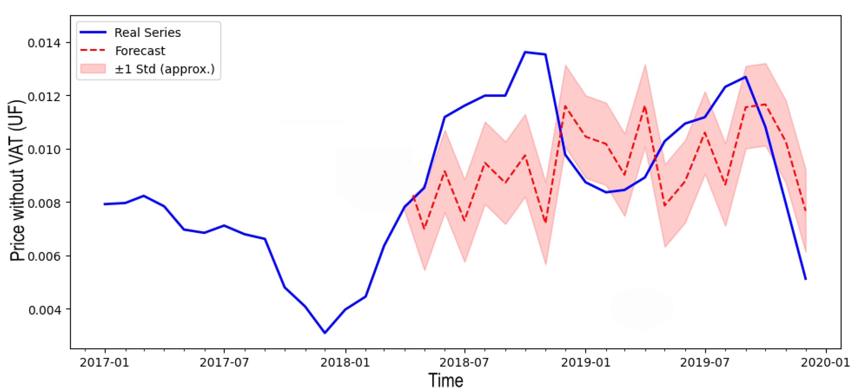
Figure 7 shows the actual price excluding VAT from 2017 to 2020 (blue line). We show the price in UF, which is a financial unit adjustable according to inflation, used in Chile. We also show the predicted values and their corresponding standard deviation, which is notably small. The results demonstrate that the predicted values closely align with the actual prices.

5. Parallel Simulation

In this work, we parallelize our proposed simulation model using an approximate optimistic approach [7]. We partition the simulation model into N logical processes (LPs), where each LP maintains a subset of entities that interact with one another.

When we parallelize the proposed simulation model, a balance problem arises. Note that the communication patterns among farmers, fairground workers, and consumers may vary depending on the products and the season. Certain fruits and vegetables are harvested at specific times of the year. In addition, not all fruits and vegetables are available year-round, and some products are more frequently consumed during hot seasons and others during cold seasons. Therefore, the communication pattern between farmers, FW, and consumers is not uniform and changes throughout the year depending on the season.

To address this problem, we use an optimistic approximate parallel simulation approach based on the Bulk Synchronous Parallel (BSP) model. In the optimistic approximate approach, precision in the results is sacrificed by ignoring the occurrence of straggler events, allowing the simulation to continue advancing while improving execution time and memory usage. In this approach, the error in the results is highly dependent on the simulation model and is controlled through mechanisms that prevent the LPs distributed across processors from advancing too far in simulation time [7].

This approach uses a time window (W), which delimits the simulation time advance in each iteration. Each LP processes and generates events autonomously until reaching the end of the time window. If, during this period, an event targeting an agent assigned to another LP arises, an outgoing message is queued to be dispatched to the destination LP. At the end of each iteration, processors are synchronized and messages are sent.

Algorithm 1 illustrates the approximate parallel simulation protocol. The input parameters are: (1) the time increment per iteration, W; (2) the parameter K, which determines how frequently the global virtual time (GVT) is updated; (3) the future event list ($FEL$); (4) the total simulation time $T_{max}$; and (5) additional configuration parameters such as the number of Logical Processes (LPs), number of processors, etc., grouped under $InputParams$. The global virtual time (GVT) is computed periodically every K iterations to determine whether all LPs have reached the simulation horizon $T_{max}$. The future event list (FEL) maintains all pending events, sorted by their times ($e.time$), which indicates when each event should be executed. In line 4, we initialize the next time window as $W_{next}=W$, meaning that during the first iteration, all events with times $\le W$ will be processed. In line 5, the main loop begins and continues either until the simulation time reaches $T_{max}$ or the FEL becomes empty (i.e., there are no more events to process). In line 6, the algorithm checks whether the local virtual time (LVT) falls within the current time window ($W_{next}$). If so, it retrieves the next event e from the FEL. In line 8, the algorithm updates the local virtual time of the LP, computed as the current value plus the execution time of the event. In other words, it advances the LP’s clock. In line 9, if the event is local, it is executed. Otherwise, it is forwarded to the corresponding LP. In line 11, the time window is incremented in preparation for the next iteration. Then, in line 12, all outgoing messages are sent. In line 13, a synchronization ensures consistency among LPs, and in line 14, incoming messages are received. The GVT is updated every K iterations, calculated as the minimum LVT across all LPs. In line 11, the time window is updated for the next iteration. Then, in line 12, the messages are sent, and finally, in line 13, synchronization occurs. In line 14, messages coming from other LPs are received, and the global virtual time $GVT$ is updated every K steps or iterations. The $GVT$ is computed as the minimum LVT of all the LPs.

Algorithm 1 General parallel simulation algorithm.

1: procedure run_parallel(InputParams, W, $T_{max}$, K, FEL) 2:     $\mathit{InitSim}\left(\mathit{InputParams}\right)$                              ▹ Initialize simulator with input parameters 3:     $S{S}_{count},LVT,GVT\leftarrow 0$ 4:     $W_{next}\leftarrow W$ 5:     while $GVT<=T_{max}$ and $!\mathit{FEL}.\mathit{empty}\left(\right)$ do 6:         while $LVT<=W_{next}$ do 7:            $e\leftarrow FEL.NextEvent\left(\right)$ 8:            $LVT\leftarrow LVT+e.time$ 9:            $\mathit{RouteEvent}\left(e\right)$          ▹ processes or queues the event for sending to another processor 10:         end while 11:         $W_{next}\leftarrow W_{next}+W$ 12:         $\mathit{SendMessages}\left(\right)$ 13:         $\mathbf{bsp}\_\mathbf{sync}\left(\right)$ 14:         $\mathit{ReceiveMessages}\left(\right)$ 15:         if $S{S}_{count}\%K==0$ then 16:            $\mathit{UpdateGVT}\left(\right)$ 17:         end if 18:     end while 19: end procedure

Load Balance Algorithm

The parallelization of the simulator developed for the case study incurs load balance and communication overheads. The sequential simulator accesses data structures located in the RAM memory to process the events related to consulting the farmers’ product stock. That is, the FW iteratively asks the farmers whether they have the products. However, in the case of the parallel simulator, the LPs are distributed among different processors, and consulting the available stock with the farmers may require several iterations, during which messages and synchronizations are required. This undoubtedly generates additional overhead that increases the execution time and causes load imbalance among the processors.

To address this problem, we propose using the simulated annealing (SA) [8] metaheuristic combined with our proposed credit algorithm. We use the SA metaheuristic to distribute the LPs among the processors. Simulated annealing (SA) is an optimization metaheuristic inspired by the annealing process in metallurgy. It explores solutions by probabilistically accepting worse solutions to escape local optima, gradually reducing this probability as the temperature decreases. The algorithm iterates until a minimum temperature is reached. We use the temporal balance objective function, which distributes the workload over multiple time periods, ensuring that all processors maintain a balanced usage at all times. To achieve this, the coefficient of variation ($CV={\displaystyle \frac{\sigma }{\mu }}$) is calculated in each period. Where $\sigma$ is the standard deviation and $\mu$ is the mean load across the partitions. If, in a given period, the mean load drops to zero (i.e., all partitions become inactive), a penalty term is introduced to further discourage the absence of work. The final objective is based on a linear combination of the balance level (measured using the CV in each period), the total workload, and penalties for inactivity.

Additionally, during the execution of the simulations, the credit algorithm works as follows. When an FW initiates a purchase with a farmer, they take a credit assuming that the purchase request will be answered favorably. In this way, transactions are not held up by waiting for the communication response from other LPs. If the response is favorable, the “credit” is cancelled. Otherwise, the FW has a debt on the product, so they cannot restart purchasing for the same product until the debt is canceled.

The credit algorithm uses a log of historical transactions between the FWs and the farmers, recording when the purchase succeeded or when a credit was granted. This information feeds a Bayesian model to estimate the response of agents residing on other processors.

Let S and F be the total number of successes and failures of the credits, respectively. That is, the number of products requested by a given farmer is successfully responded to or not. The prior probability of success is defined using the Laplace formulae:

$$P\left(s\right)={\displaystyle \frac{S+\alpha }{S+F+2\alpha }},P\left(f\right)=1-P\left(s\right)={\displaystyle \frac{F+\alpha }{S+F+2\alpha }},$$

(4)

where $\alpha$ is a parameter used to adjust observed data counts, effectively addressing the issue of zero-frequency values in categorical data. Setting $\alpha =1$ corresponds to Laplace’s rule of succession, which assumes a uniform prior distribution over all possible events or categories, thereby ensuring that every outcome has a non-zero probability.

For each product i, $S_i$ successes and $F_i$ failures are counted, and for each process j, $s_j$ successes and $f_j$ failures are counted. $\alpha$ is the smoothing parameter, usually set to 1. The conditional probabilities are defined as:

$$P(s\mid {\mathrm{product}}_i)={\displaystyle \frac{S_i+\alpha }{S+2\alpha }},P(f\mid {\mathrm{product}}_i)={\displaystyle \frac{F_i+\alpha }{F+2\alpha }},$$

(5)

$$P(s\mid {\mathrm{process}}_j)={\displaystyle \frac{s_j+\alpha }{S+2\alpha }},P(f\mid {\mathrm{process}}_j)={\displaystyle \frac{f_j+\alpha }{F+2\alpha }}.$$

(6)

We assume that given the state (success or failure), the product and process variables are independent. Thus, the likelihoods for success and failure are defined as:

$$L(s\mid i,j)=P\left(s\right)P(s\mid {\mathrm{product}}_i)P(s\mid {\mathrm{process}}_j),$$

(7)

$$L(f\mid i,j)=P\left(f\right)P(f\mid {\mathrm{product}}_i)P(f\mid {\mathrm{process}}_j).$$

(8)

Finally, applying Bayes’ theorem, the predictive probability of success for the pair $({\mathrm{product}}_i,{\mathrm{process}}_j)$ is computed as:

$$P(s\mid i,j)={\displaystyle \frac{P\left(s\right)P(s\mid {\mathrm{product}}_i)P(s\mid {\mathrm{process}}_j)}{P\left(s\right)P(s\mid {\mathrm{product}}_i)P(s\mid {\mathrm{process}}_j)+P\left(f\right)P(f\mid {\mathrm{product}}_i)P(f\mid {\mathrm{process}}_j)}}.$$

(9)

This probability determines whether a message is sent to another LP and credit is granted to the agent initiating the purchase process. If the estimate is unfavourable, it is assumed that the purchase process will not be successful, and the purchase is canceled. Therefore, the FW selects another farmer to buy the product.

6. Experiments

We perform all experiments with 14,375 FWs, 4695 farmers, and 29,394 consumers for the metropolitan city of Santiago. In the case of the sixth region of Chile, we use 10,284 FWs, 4863 farmers, and 20,568 consumers. To determine the products to be consumed and their quantities, we use the information available in the National Food Consumption Survey that studies consumption patterns in Chileans [38]. In addition, we assume a family budget dedicated to purchases at free markets, ranging from 25,000 to 45,000 Chilean Pesos (CLP). This data was obtained from [39]. We run the experiments on a multicore processor with 32 processors, a 4-bit Intel Core Q9550 2.83GHz, and 64GB of RAM DDR3 1333 MHz.

Multiple experiments were conducted for the agent configurations described in

Table 5. Simulation configurations for different types of farmers, fairgoers, and consumers.

Config ID	Farmer Type	FW Type	Customer Type
1	simple	static	simple
2	simple	static	family
3	simple	static	family budget
4	simple	seasonal	simple
5	simple	seasonal	family
6	simple	seasonal	family budget
7	simple	proportional	simple
8	simple	proportional	family
9	simple	proportional	family budget
10	finance	proportional	simple
11	finance	proportional	family
12	finance	proportional	family budget
13	risk	static	simple
14	risk	static	family
15	risk	static	family budget
16	risk	seasonal	simple
17	risk	seasonal	family
18	risk	proportional	simple
19	risk	seasonal	family budget
20	risk	proportional	family
21	risk	proportional	family budget

. We excluded the configurations involving $\left\{finance\right\}\times \{static, seasonal\}\times \{simple, family, familybudget\}$, as they consistently yielded Mean Absolute Percentage Error (MAPE) values close to 1, indicating poor predictive performance.

6.1. Simulation Model Accuracy Evaluation

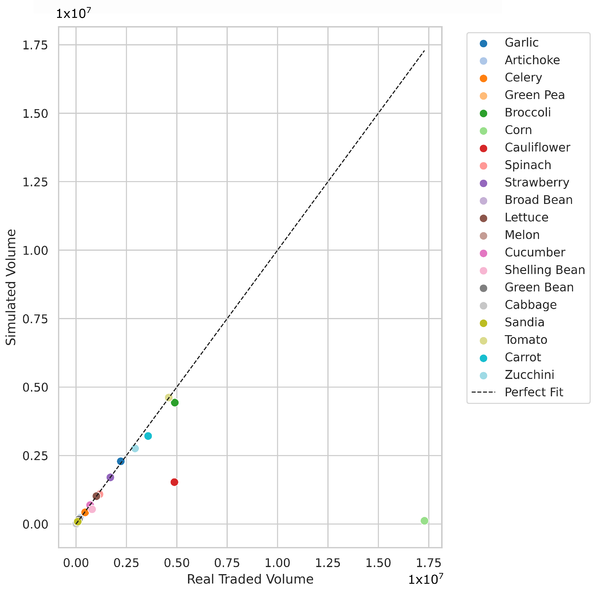
Figure 8 and Figure 9 illustrate the total number of products sold reported by our simulator and in the National Food Consumption Survey, which studies consumption patterns in Chilean people [38]. Figure 8 shows results for the metropolitan city of Santiago and Figure 9 shows the results obtained for the sixth region of Chile. The dotted line represents the case where the simulation reports the same number of products sold as the real data. Results show that most products are close to the dotted line. Only corn shows a greater difference than the simulated case.

Figure 10 shows the Mean Absolute Percentage Error (MAPE) for different simulation configurations. That is when the simulator is executed with different combinations of farmers (simple, finance, risk), FWs (static, seasonal, proportional), and consumers (simple, family, family budget). Figure 10a shows results for the metropolitan city of Santiago, and Figure 10b shows the results obtained for the sixth region of Chile. Results show that the MAPE is below 11% in all cases, demonstrating that our simulator can reproduce the real values with a small error.

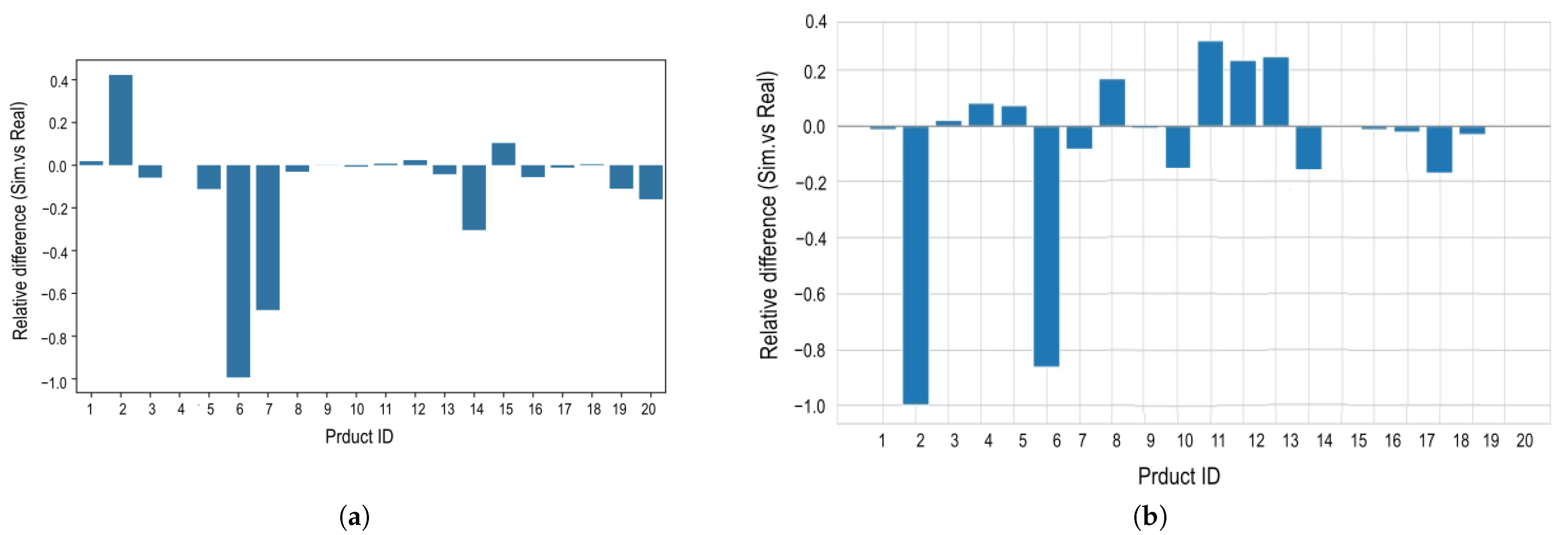
Figure 11 shows the relative difference in traded volumes for all simulated products. Figure 11a shows results for the metropolitan city of Santiago and Figure 11b for the sixth region of Chile. The results show that most products can be simulated with high accuracy, with relative differences of less than 1%. Products such as corn ($x=6$) and cauliflower ($x=7$) are underrepresented, indicating that fewer transactions were simulated than expected for the metropolitan city of Santiago. Artichokes ($x=2$) are overrepresented in the simulated traded volumes, as this product reports a lower purchase volume per vendor, which makes it easier for purchase requests to be fulfilled. In the case of the sixth region of Chile, Artichokes ($x=2$) and corn ($x=6$) are underrepresented, meanwhile lettuce ($x=11$), melon ($x=12$), and cucumber ($x=113$) are overrepresented.

6.2. Analysis of Environmental Risk Factors

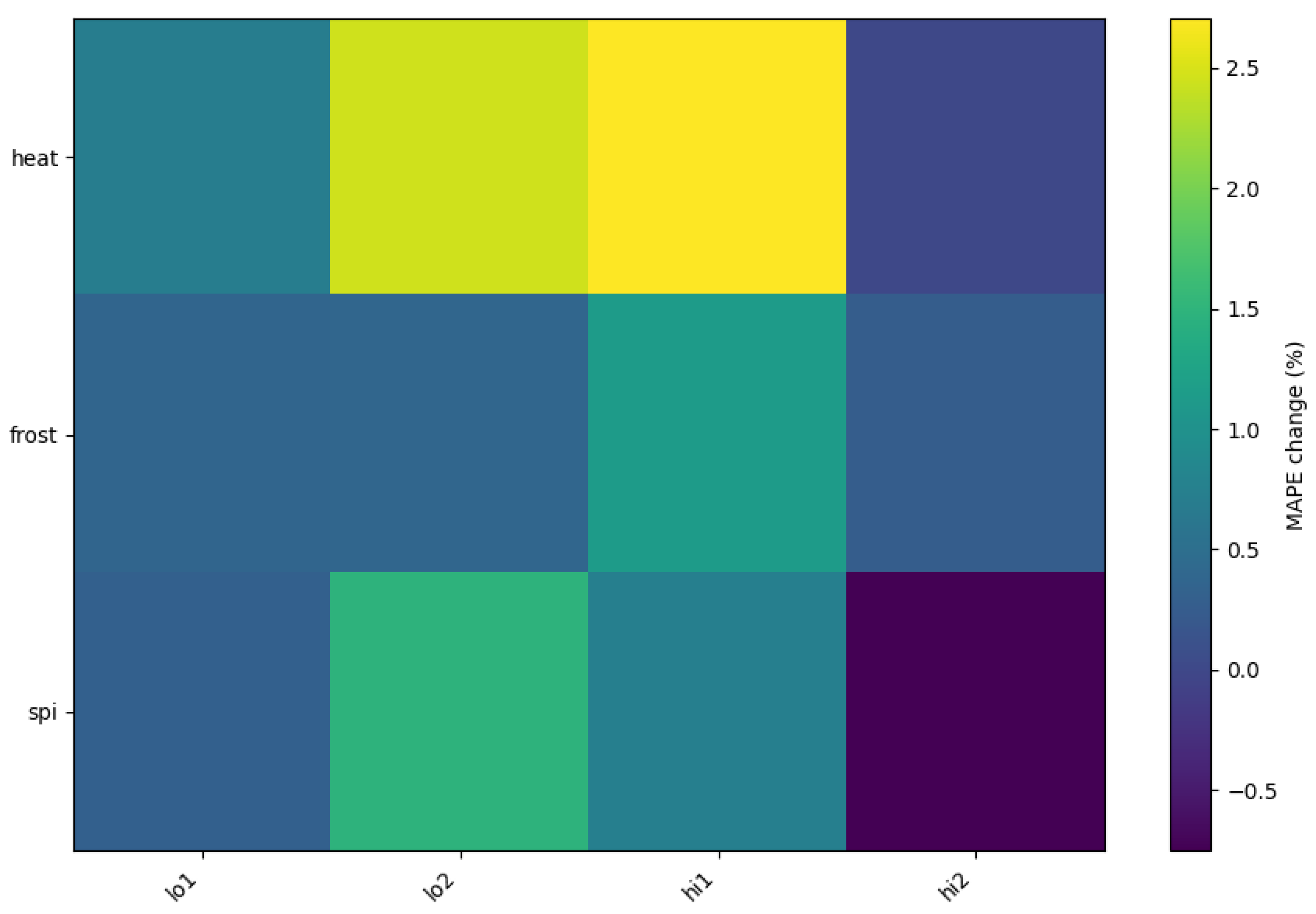
In this section, we analyze the sensitivity of the environmental risk factors such as frosts, droughts, and heatwaves. Figure 12 presents a heatmap showing the percentage variation in the Mean Absolute Percentage Error (MAPE) under different stress test scenarios for environmental risk parameters. The rows represent the three risk dimensions considered in the model—heatwaves, frosts, and droughts (measured via the Standardized Precipitation Index, SPI)—while the columns correspond to scenario intensities: low 1 (lo1), low 2 (lo2), high 1 (hi1), and high 2 (hi2). Each scenario was evaluated while holding all other factors constant (ceteris paribus), modifying only the target variable’s intensity across months. For instance, in the hi2 heatwave scenario, each month was increased by two intensity levels, whereas in the lo1 frost scenario, one level was subtracted per month.

Regarding the heatwave, the MAPE increased substantially in the hi1 and lo2 scenarios, with the highest variation reaching over 2.5% in hi1. This indicates that the model is particularly sensitive to increases in heatwave intensity. Interestingly, reducing heatwave levels (lo1) also increased MAPE slightly, suggesting that both extreme increases and decreases affect the prediction accuracy. The hi2 scenario shows a smaller impact than hi1, possibly due to saturation or threshold effects in the model’s sensitivity.

By evaluating the frosts, the model shows moderate sensitivity to changes in frost intensity. The largest increase in MAPE occurs under the hi1 condition, but remains below 1.5%. The low-impact scenarios (lo1 and lo2) have a minimal effect, suggesting that parameter sensitivity is relatively stable against slight reductions in frost intensity.

Finally, when evaluating the frosts, a notable variation is observed in lo2, with an MAPE increase close to 1.5%, indicating that the parameter is sensitive to reductions in precipitation (more drought-prone scenarios).

6.3. Parallel Simulator Assessment

We run the parallel experiments with the configuration $\#19$, which reported the best MAPE results.

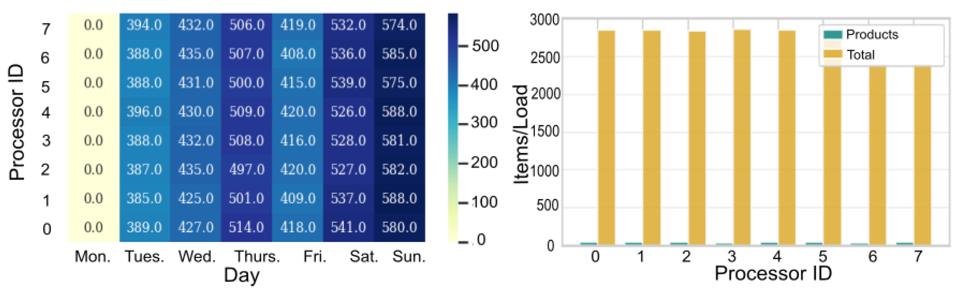
In Figure 13, we show the results obtained by the Simulated Annealing metaheuristic when the simulator is executed in $P=8$ processors. At left, we show the workload reported by each processor. The workload distribution per simulated day and per processor is homogeneous across partitions (processors 0 to 7), although it varies from day to day. Notice that there is no workload on Mondays. This is correct, as open fairs do not operate on the first day of the week. At right, we show the number of product items (open-fairs, farmers, FWs, consumers) assigned to each processor. The orange bars show the average number of items assigned to the processors over the months, and in green, the number of products assigned to each processor. This graph shows that the distribution is similar for each processor.

In the following experiments, we show the results achieved with the baseline simulator (without the credit load balance algorithm) and the credit-based simulator. Additionally, we implemented two versions of the parallel and the sequential simulators. The first one executes atomic events for each task detailed in Figure 1. In the second version, the events associated with the tasks “Purchase between fairground workers and farmers” and “Purchase between fairground workers and customers” are grouped into a single event. This is because using the atomic version, the number of events can easily exceed 300 million; meanwhile, with the grouped version, the number of events averages around 4.3 million.

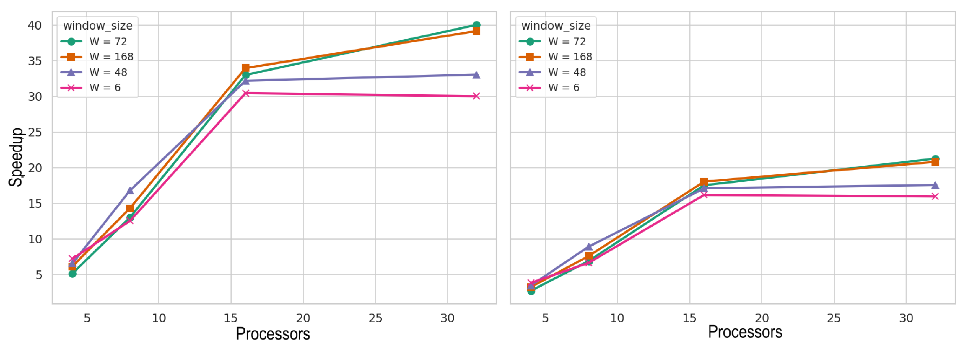
Figure 14 and Figure 15 show the speedup obtained for the baseline parallel simulator when running the atomic (left) and the grouped (right) versions for the metropolitan city of Santiago and the sixth region of Chile, respectively. The x axis shows the number of processors. In both cases, the speedup tends to improve with a greater number of processors. Experiments executed with $W=48$ for the metropolitan city of Santiago produce better results. In the case of the sixth region of Chile, results obtained with $W=48$ report good speedup, but the best speedup is obtained with $W=6$ and $W=24$ with 16 processors. This is because the sixth region involves a smaller number of simulated agents. As a result, increasing the number of processors does not lead to a significant speedup, since the workload is not large enough to fully utilize the available computational resources. 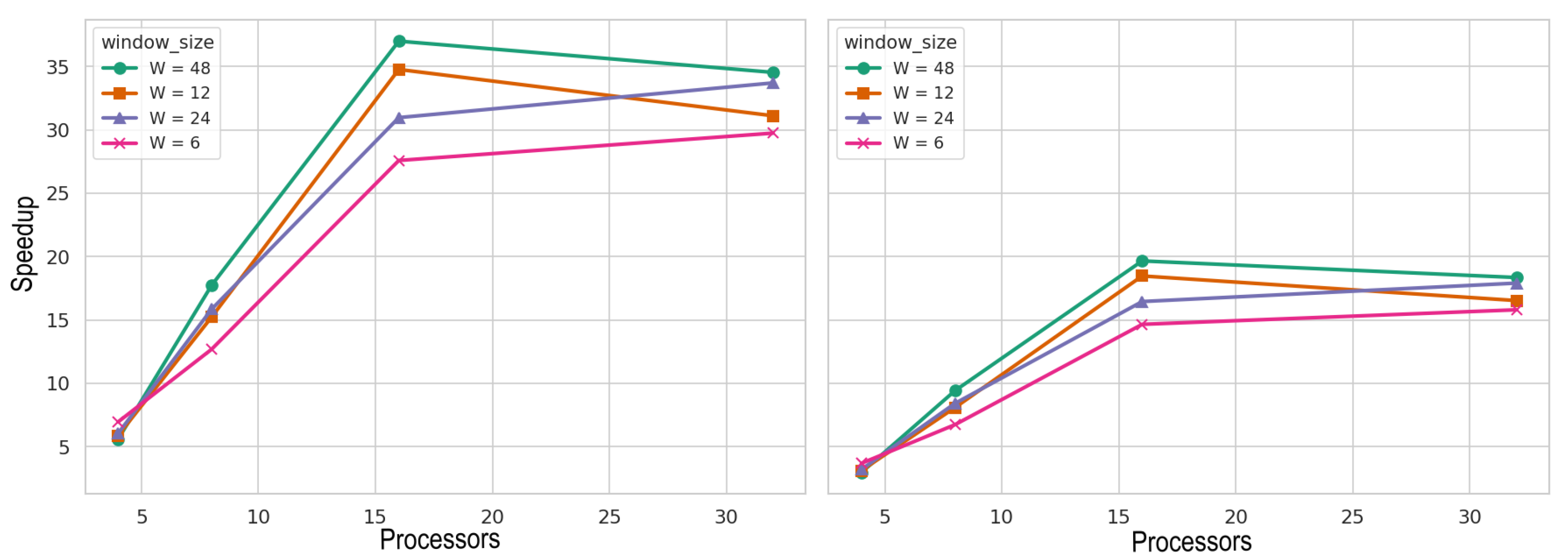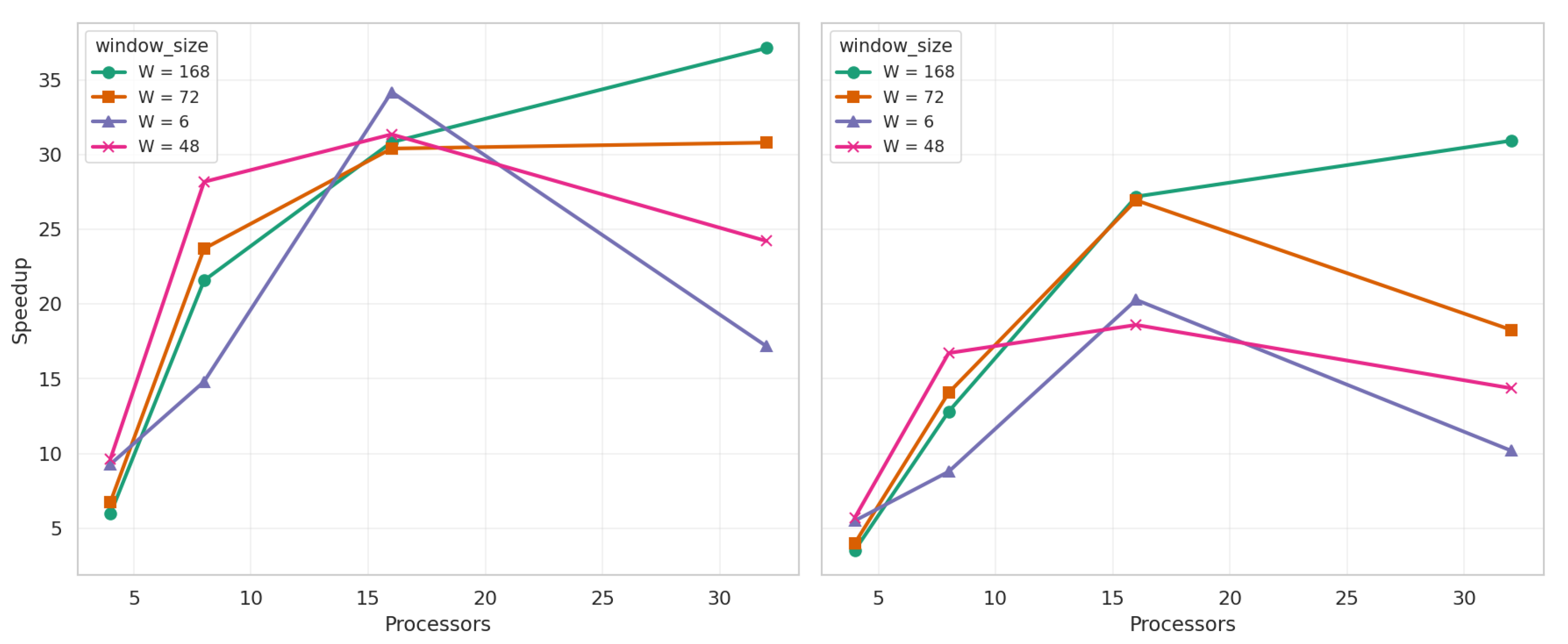Figure 16 and Figure 17 show the speedup for the credit-based parallel algorithm when running the atomic (left) and the grouped (right) versions for the metropolitan city of Santiago and the sixth region of Chile, respectively. In the first case, the values $W=72$ and $W=168$ report the best speedups when using more than 16 processors. With fewer processors, the results tend to be similar, with a slight advantage when using $W=45$. The results for the sixth region indicate that for $P\le 16$, using $W=48$ yields a good speedup. However, when scaling up to $P=32$, the best speedup is achieved with $W=168$. This is primarily because the amount of work on each processor is reduced, and a larger time window decreases the overall number of synchronization operations across processors. Additionally, the credit-based algorithm tends to reduce the number of executed iterations, as it assumes that farmers will have the requested quantity of products. If this assumption is not fulfilled, the farmer is simply penalized by receiving fewer products in the future. In contrast, the baseline algorithm always ensures that farmers have the required quantities before processing a purchase, which demands more communication and a greater number of iterations.

When simulating a large number of agents, as in the case of the metropolitan city of Santiago, both the baseline and the credit-based parallel simulators tend to yield similar results when using a small number of processors ($P\le 16$). However, the credit-based algorithm significantly improves the speedup for P = 32 (see

Table 6. Speedup reported by the parallel simulators.

	Santiago (P = 32)		Sixth Region (P = 16)		Sixth Region (P = 32)
	Atomic	Grouped	Atomic	Grouped	Atomic	Grouped
Credit	38.7	23.4	33.8	26.6	36.1	30.8
Baseline	34.1	18.7	34.3	20.1	24.2	14.8

). Furthermore, all algorithms present near-linear speedup for $P\le 16$. Although each iteration imposes a global barrier, message traffic remains regular, and load imbalance is limited. Additionally, with 20 products, each processor operates on a local FEL of approximate size $N/P$. Since operations on a heap (the data structure used to implement the FEL) have a complexity of $\mathcal{O}(logn)$, the time required for insertion or extraction is reduced from $logN$ to $log(N/P)$. Combined with the lower synchronization frequency characteristic of the credit-based algorithm, this algorithmic efficiency results in a superlinear speedup.

For $P>16$, the number of processors exceeds the number of products, introducing imbalance and causing the speedup curve to flatten or even decrease. This effect is more drastic in the case of the sixth region, which involves a smaller number of simulated agents. However, the use of barriers prevents lightweight processors from becoming completely idle, and the overhead introduced by the credit-based scheme helps avoid unnecessary communication.

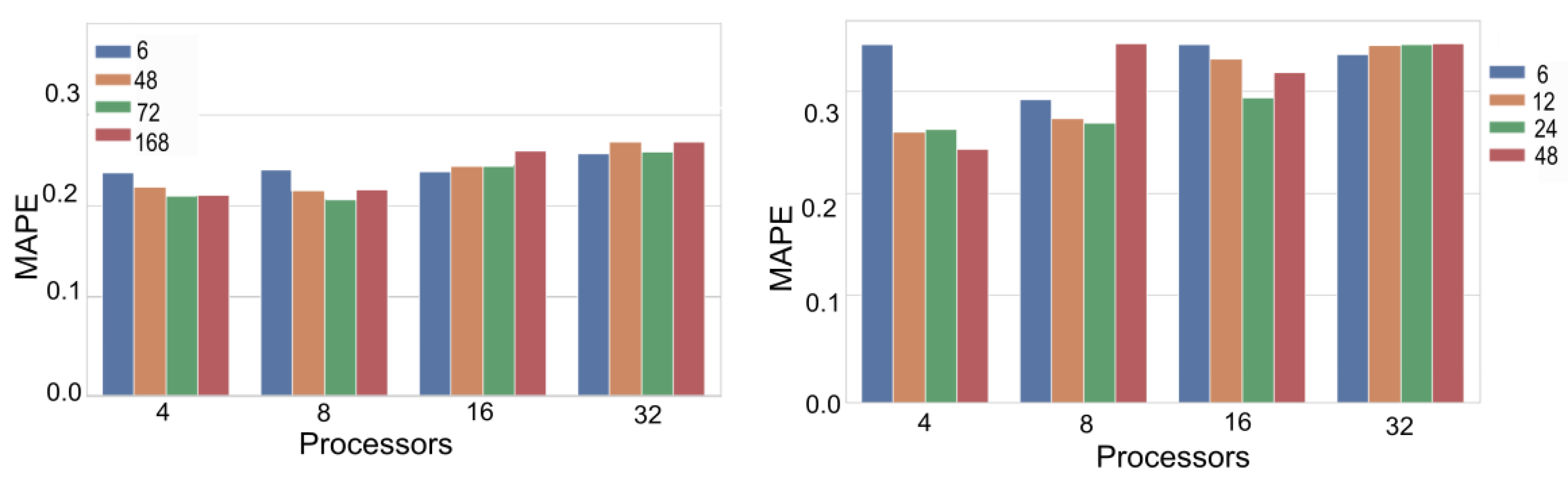
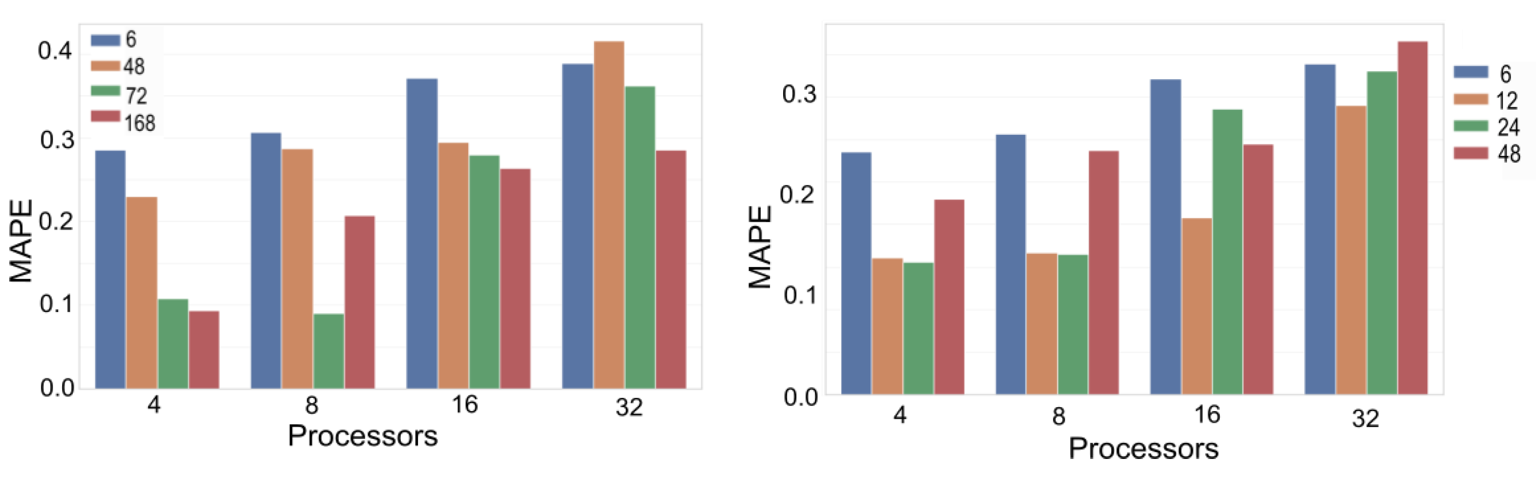
Figure 18 shows the MAPE error of the proposed credit-based parallel simulator (left) and the baseline parallel simulator (right) for the metropolitan city of Chile. As expected, the error tends to increase with a larger number of processors. Results show that our proposal can reduce the error reported by the baseline parallel simulator. The proposal keeps the error below 27% meanwhile the baseline reports errors close to 38%. In Figure 19, we show the results obtained for the sixth region of Chile. Similar to the previous case, our proposal reports lower MAPE values than the baseline for $P=4$ and $P=8$. For $P\ge 16$, the baseline exhibits slightly lower MAPE values.

7. Discussion

The development of simulation tools for analyzing urban agricultural supply chains presents significant challenges, particularly in terms of balancing model complexity, data availability, computational demands, and real-world applicability. Our proposed framework, which integrates agent-based modeling (ABM) with discrete event simulation (DES) and incorporates an approximate optimistic parallel execution strategy, represents a step forward in tackling these challenges.

While our simulator captures key decision-making dynamics among farmers, vendors, and consumers, we acknowledge the inherent trade-offs in behavioral modeling. Real-world consumer behavior is influenced by a wide range of factors—cultural, economic, and situational—which are difficult to capture in their entirety, particularly when working with limited or aggregated data. To mitigate this, we implemented a range of agent profiles (e.g., risk-aware farmers, seasonal fairground workers, and family budget consumers) that allow for more complex behaviors than purely random or rule-based actions. Nonetheless, we recognize the value of further sophistication and have identified this as a priority for future work, including the exploration of reinforcement learning techniques to enable adaptive and evolving behaviors.

A major limitation in modeling informal or semi-formal food markets is the scarcity of fine-grained, high-resolution datasets—particularly concerning purchasing patterns and household-level consumption dynamics. To address this, we relied on the most complete data sources available for Santiago, Chile, and the sixth region of Chile, including historical price data and national consumption surveys.

A recurrent concern in deploying complex simulation systems is the technical barrier to entry. While our simulator was evaluated on a 32-core machine to assess performance under large-scale configurations, the framework supports both sequential and optimized low-cost parallel executions. The dual implementation of atomic and grouped event strategies enables users to adjust the level of computational granularity according to their hardware capacity. Additionally, the model’s modular design and configuration files allow for easy customization without modifying the source code, thus reducing the expertise required for its use.

8. Conclusions

In this work, we present a simulator tool that combines ABS and DES to model and analyze vegetable trade dynamics. We evaluated our proposal using two use cases—the metropolitan city of Santiago and the sixth region of Chile. By integrating agent interactions among farmers, fairground workers, and consumers, our approach captures key decision-making processes in the supply chain, reflecting the real-world complexities of agricultural markets. Our proposal successfully combines the strengths of agent-based and discrete event simulation, enabling a more realistic and granular representation of trade interactions, supply chain fluctuations, and agent behavior in agricultural markets.

Additionally, we parallelize our proposal using an optimistic approximate approach to address the computational demands of large-scale simulations. This method reduces execution time. To tackle the load imbalance produced by the heterogeneous communication patterns, we present a credit-based algorithm, which enhances performance and scalability in multi-agent trade simulations.

Our experimental results show that the proposed hybrid simulation model effectively reduces computational overhead and improves execution efficiency. The integration of an adaptive load balancing mechanism further optimizes resource allocation, ensuring stable and efficient simulation performance.

In future work, we plan to improve the agent behavior models via learning and data-driven strategies. In particular, we plan to explore reinforcement learning techniques to enable adaptive decision-making for farmers and vendors based on evolving market conditions. We also plan to extend our research to additional geographic regions and products, as well as to integrate the framework with real-time or streaming data to enhance predictive and decision-support capabilities.