Abstract
Federated learning (FL) has emerged as a powerful approach for privacy-preserving model training in autonomous vehicle networks, where real-world deployments rely on multiple roadside units (RSUs) serving heterogeneous clients with intermittent connectivity. While most research focuses on single-server or hierarchical cloud-based FL, multi-server FL can alleviate the communication bottlenecks of traditional setups. To this end, we propose an edge-based, multi-server FL (MS-FL) framework that combines performance-driven aggregation at each server—including statistical weighting of peer updates and outlier mitigation—with an application layer handover protocol that preserves model updates when vehicles move between RSU coverage areas. We evaluate MS-FL on both MNIST and GTSRB benchmarks under shard- and Dirichlet-based non-IID splits, comparing it against single-server FL and a two-layer edge-plus-cloud baseline. Over multiple communication rounds, MS-FL with the Statistical Performance-Aware Aggregation method and Dynamic Weighted Averaging Aggregation achieved up to a 20-percentage-point improvement in accuracy and consistent gains in precision, recall, and F1-score (95% confidence), while matching the low latency of edge-only schemes and avoiding the extra model transfer delays of cloud-based aggregation. These results demonstrate that coordinated cooperation among servers based on model quality and seamless handovers can accelerate convergence, mitigate data heterogeneity, and deliver robust, privacy-aware learning in connected vehicle environments.
1. Introduction
Autonomous driving (AD) combines advanced sensing, high-performance computing, and artificial intelligence (AI) to perceive the environment and make control decisions without human intervention, substantially reducing the number of collisions caused by drivers’ errors. At its core, machine learning (ML)—especially deep neural networks—powers essential autonomous functions such as object detection, semantic segmentation, and path planning by extracting rich, hierarchical features from camera, LiDAR, and RADAR data [1].
Modern vehicles are estimated to generate enormous volumes of raw sensor data—up to one gigabyte per vehicle per second [2]—and are increasingly interconnected via vehicle-to-everything (V2X) links [3]. As connected vehicles become more prevalent, vehicular operations are expected to rely not only on locally collected data, but also on shared sensor data across networks of interconnected vehicles [3]. Future autonomous vehicles will perceive their environment through built-in sensors and share this information with other vehicles via wireless communications, collecting substantial amounts of data for distribution [1]. Sharing sensor data is critical for safety applications, such as creating high-definition maps, and for developing ML models that perform autonomous driving tasks like speed adjustment, steering, and traffic sign recognition [4].
Traditionally, vehicular networks have relied on a centralized learning (CL) paradigm: raw sensor outputs are uploaded to a cloud, where powerful ML models—typically deep neural networks—are trained to map inputs (e.g., images, point clouds) to driving outputs (e.g., steering angles, object classes), and the resulting global model is then pushed back to vehicles for on-board inference. However, CL’s dependence on continuous, large-scale data transmission can overwhelm the network bandwidth, introduce latency that undermines safety-critical response times, and expose sensitive sensor data [1]. The widespread distribution of sensor data also raises serious privacy concerns, as it can reveal confidential information about vehicles and occupants. While privacy issues related to sharing vehicle status data have been addressed through methods like data anonymization, these measures have not been fully applied to sensor data sharing [3]. Moreover, conventional data anonymization techniques have seen limited application to high-volume, high-fidelity sensor streams, leaving significant privacy gaps.
To mitigate privacy concerns, federated learning (FL) [5,6] has emerged as a promising solution, enabling clients (e.g., vehicles) to collaboratively develop ML models without sharing confidential raw data. In FL, a server shares the initial model parameters with clients, who train the model on local datasets and return updated parameters. The server aggregates these updates to create a global model, iterating until a predefined level of accuracy is achieved. Since FL is trained on distributed datasets and typically involves numerous communication rounds between clients and the central server to exchange model updates, two major challenges have emerged and attracted significant research focus: improving communication efficiency between clients and the central server and addressing the heterogeneous distribution of local datasets across clients [6].
Existing research on FL has traditionally focused on single-server architectures, where clients repeatedly exchange model updates with a centralized server during each communication round. This interaction strategy can introduce significant communication delays, especially in large-scale FL scenarios where numerous clients may be geographically distant from the central server—delays that are exacerbated when the central server is deployed in the cloud. Moreover, real-world vehicular networks often involve multiple access points, each with its own server, yet previous studies [7,8,9] on FL in vehicular networks have primarily emphasized client-side operations. While the server plays a critical role in orchestrating the learning process by aggregating local model updates and ensuring data privacy and system security, the potential of multi-server architectures—particularly when explicitly considering server performance metrics such as accuracy and loss—remains underexplored.
Given the rising prevalence of delay-sensitive applications, especially in autonomous driving and wearable health monitoring, recent studies have proposed multi-server FL architectures. To effectively reduce the communication latency inherent in traditional FL, two primary multi-server approaches have been explored: (1) hierarchical FL (HFL) [10,11,12,13] and (2) clustered FL (CFL) [14,15,16,17]. HFL adopts a layered structure in which multiple edge servers independently aggregate local model updates from clients within their coverage areas. These edge servers then forward their aggregated models to a central cloud server for global aggregation. However, as model exchanges between edge servers and the cloud server are still necessary, HFL may still experience substantial training delays, especially when the propagation delay between edge servers and the cloud server is considerable. CFL partitions clients into distinct clusters, each training a separate machine learning model. Nevertheless, dynamic re-clustering may be required across multiple communication rounds, significantly increasing computational complexity and overall training time [18,19].
In this paper, we present a novel MS-FL framework specifically designed for vehicular networks, aligning seamlessly with the vehicular edge computing (VEC) architecture by leveraging RSU resources to accelerate ML model training. In this framework, FL servers deployed at RSUs collaboratively exchange and evaluate trained models using multi-cast communication, thereby reducing the network overhead. This collaboration enables quality-driven model exchange, granting greater weight to more reliable contributions and thus accelerating global convergence. The contributions of this paper can be summarized as follows:
- We propose a novel multi-server framework at the RSU level, enabling peer servers to share model updates among neighboring servers. By leveraging inter-RSU collaboration, our framework accelerates convergence and enhances robustness in highly mobile vehicular networks;
- We develop and evaluate server-level, performance-based aggregation strategies whereby each FL server first assesses incoming peer models’ accuracy and loss against its own validation data and then selectively incorporates these updates. Empirical results demonstrate that these performance-driven methods consistently outperform standard baselines. We also employ a statistical model to penalize outliers and reduce the impact of contributions from servers whose data or model updates deviate significantly from the expected behavior. These deviations, or “outliers”, may indicate malicious activity, faulty data, or other anomalous behaviors;
- We propose an inter-server handover mechanism for continuous FL that preserves updates that would otherwise be lost as vehicles traverse multiple servers, leveraging migrating clients to accelerate global convergence. Our approach also incorporates a server-side evaluation module that assesses and weights each newly arrived client’s update—taking into account its origin server—before integrating it into the global model aggregation;
- We show via experiments that our solution provides remarkable performance gains compared to (1) baseline FL at each server, where servers train and aggregate only their own local updates (no inter-server collaboration), referred to as “single-server FL” in this paper; (2) hierarchical FL with cloud synchronization, in which servers periodically send models to—and receive updates from—a central cloud server (incurring a high communication overhead), referred to as “cloud-based FL” in this paper; and (3) methods that do not take model handover between servers into account.
The remainder of this paper is organized as follows. Section 2 reviews recent related work. Section 3 presents our system model and problem definition. In Section 4, we introduce the proposed multi-server FL framework, detailing the server-level evaluation and aggregation algorithms as well as the handover mechanism. Section 5 analyzes the transmission latency of various FL frameworks. The simulation setup and results are discussed in Section 6. Section 7 offers a broader discussion of our findings and outlines directions for future work.
2. Related Work
Federated learning is a new machine learning paradigm that tries to address data privacy concerns in a multi-federated environment, where multiple servers share their training models, and not raw data, in an effort to build a consensus on a global model. Below, we review the prior work most relevant to our study, organized into two categories: multi-server federated learning in general, and multi-server federated learning specifically in vehicular networks.
2.1. Multi-Server Federated Learning
Han et al. [18] propose FedMes, a federated learning framework specifically tailored for cellular networks with multiple edge servers. In conventional edge-based FL, individual edge servers are often hampered by limited client populations and biased data distributions due to their restricted coverage areas. FedMes overcomes these challenges by exploiting the overlapping regions between adjacent edge servers. In these overlapping areas, clients receive models from multiple servers and average them, effectively serving as conduits that synchronize and disseminate updated models across servers, thereby reducing latency and improving convergence in practical deployments.
In a similar vein, Qu et al. [19] introduce MS-FedAvg, another multi-server FL framework that leverages overlapping coverage among regional servers to facilitate model sharing without a central aggregator. In MS-FedAvg, clients situated in overlapping regions download several regional models and compute an initial averaged model before performing local updates via standard SGD. Regional servers then update their models based on these client updates, and the final global model is obtained by aggregating the regional models after a fixed number of communication rounds. While both approaches exploit overlapping areas, MS-FedAvg distinguishes itself by providing a thorough convergence analysis under non-convex settings and by incorporating algorithmic refinements—such as biased client sampling—to enhance both theoretical guarantees and empirical performance in heterogeneous network environments. Despite these promising strategies, both FedMes and MS-FedAvg rely on devices in overlapping regions to act as intermediaries. A potential concern is that since the same devices participate in training across multiple edges, their local models are recalculated by different servers. This can lead to biased updates that may adversely affect the overall global model if not carefully managed.
Rjoub et al. [20] has investigated multi-server federated learning architectures for healthcare applications, such as COVID-19 detection, using IoT devices. In these architectures, knowledge is shared across multiple servers, providing benefits like quicker data access and mitigating the issue of limited data on individual devices. However, these studies do not account for the reliability of the shared knowledge, which could lead to significant declines in global model accuracy if unsuitable models are shared between servers.
2.2. Multi-Server Federated Learning in Vehicular Networks
Taik et al. [17] propose a clustered architecture for vehicular federated learning that integrates both learning and scheduling mechanisms to address the unique challenges of vehicular networks. Their framework leverages vehicular-to-vehicular (V2V) communication to mitigate communication constraints, enabling clusters of vehicles to train models concurrently. In each cluster, vehicles collaborate locally by aggregating their model updates, and only the aggregated output is transmitted to a multi-access edge computing (MEC) server for further global aggregation. This clustered approach not only supports both single-task and multi-task learning, but also accounts for critical factors such as data heterogeneity and mobility constraints. Although the design emphasizes client-side operations and efficient intra-cluster cooperation, its reliance on a centralized MEC server for final aggregation distinguishes it from fully decentralized models, potentially impacting scalability in more dynamic scenarios.
Zhou et al. [10] introduced a two-layer federated learning architecture for the 6G-enabled Internet of Vehicles (IoV), where a central cloud server aggregates model parameters from RSUs based on their contextual information, such as vehicle locations and computational power. At the RSU level, local models from vehicles are aggregated using a weighted mechanism that prioritizes data from nearby vehicles with higher-quality contributions. The cloud server then performs global aggregation, improving model accuracy and convergence speed. While this framework enhances learning efficiency, it relies heavily on frequent communication with the central cloud server, which may introduce latency and centralization bottlenecks.
The authors in [21] proposed a trust-based knowledge-sharing mechanism within a multi-server FL architecture. In this approach, each server calculates trust scores for other servers based on the feedback received from its clients. This method demonstrated improved accuracy and reduced loss, particularly during the initial training rounds. However, the framework selects only one global model for the subsequent training round based on the highest trust score, potentially overlooking valuable contributions from other servers. This limitation can be critical in vehicular networks with non-IID data, where diverse contributions from multiple servers may be necessary to improve the overall model performance.
2.3. Research Gap
Most prior studies focused on single-server FL, cluster-based architectures [17], or cloud-centric designs [10]. A few multi-server FL approaches have been proposed, but they target relatively static environments (e.g., cellular edge servers [18,19] or IoT healthcare scenarios [20]) and do not account for the high mobility and dynamic nature of vehicular networks.
Existing multi-server schemes generally aggregate all received model updates without evaluating their quality. In a dynamic vehicular setting, outdated or compromised updates from peer servers can introduce bias, slow convergence, or even degrade the global model’s accuracy. Prior work on trust-based multi-server frameworks [21] selects only the single “most trusted” model from clients’ perspectives, potentially discarding useful diversity.
Moreover, vehicular clients frequently enter and leave RSU coverage areas, causing non-IID data distributions and uneven update rates. Yet, most multi-server FL frameworks assume stable client populations or rely on static overlap regions for model exchange, overlooking the impact of vehicle mobility on training consistency and convergence.
We introduce MS-FL, a multi-server FL framework for vehicular edge networks. First, each server shares its model with neighboring servers and vehicles, enabling efficient peer-to-peer model exchange across overlapping coverage areas and distributing the current model to vehicles for local training. Next, every server evaluates incoming peer updates on its own validation set, filters outliers, and weights each contribution by its assessed quality before aggregation. Finally, our handover protocol preserves any “lost” updates—when a vehicle crosses into a new server’s coverage, it forwards its pending update rather than dropping it. Together, these mechanisms dynamically adapt to changing client populations, reduce bias from stale or anomalous updates, and integrate multiple reliable models in each round—yielding faster convergence, higher accuracy, and greater robustness in vehicular scenarios.
Table 1 provides a concise comparison of representative FL schemes. We contrast traditional single-server FL, hierarchical FL, and two prior edge-only multi-server approaches [18,21] against our proposed MS-FL framework. Key dimensions of comparison include the communication topology (edge-only vs. edge + cloud), support for client handover, whether models are evaluated before aggregation, and whether aggregation occurs at the server level. For each method, we also summarize its primary advantages and limitations in handling non-IID data, client dropout, overlapping coverage, and end-to-end latency.

Table 1.
Comparison of FL methods. The table contrasts key features—communication latency, support for model handover, and the presence of pre-aggregation evaluation and server-level aggregation—alongside each method’s strengths and weaknesses.
3. System Model and Problem Definition
3.1. System Model
This section outlines the fundamental architecture of the vehicular network under investigation. The system consists of two main components:
- A set of RSUs., each hosting an FL server.
- A set of vehicles across RSUs.
In VEC, RSUs serve as edge servers strategically positioned along roadways, serving as access points that provide extensive communication, computational, and storage resources compared to vehicles. RSUs are responsible for identifying nearby vehicles, aggregating model updates from both vehicles and peer RSUs, and managing overall network operations. Communication between vehicles and RSUs occurs over wireless links and cellular technologies (e.g., 5G, 6G), while RSUs connect to the internet via reliable backhaul links [22,23].
Each vehicle is equipped with advanced communication interfaces that enable Vehicle-to-RSU (V2R) communication, robust onboard computing and storage resources for local processing and training, and a variety of sensors, such as cameras, radars, and GPS that allow it to monitor both internal diagnostics (e.g., engine performance, GPS data) and external conditions (e.g., road status, traffic, environmental data). Vehicles act as data collectors by continuously gathering critical information from both their onboard systems and external environments. This sensor data is then used to train and update machine learning models, typically neural networks that perform essential tasks such as object detection, image classification, and route optimization. By integrating diverse data sources, these models significantly enhance real-time decision-making, ultimately improving driving safety and operational efficiency.
To capture the system dynamics, the network’s operation is divided into discrete time intervals, . At each time step, the system undergoes a series of interactions. The data collected using vehicle during time step is represented as , while the state of the machine learning model within vehicle at the end of that time step is denoted by , the model’s parameters. The state of the machine learning model within server at the end of time step is represented by . An overview of the vehicular network with multiple servers is illustrated in Figure 1.
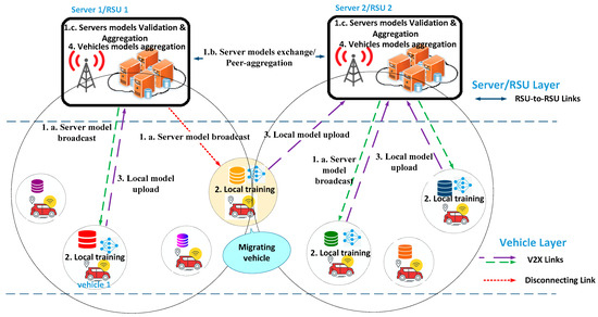
Figure 1.
System model for multi-server FL in vehicular edge computing. Each server broadcasts its global model to nearby vehicles that perform local training and upload their updates via V2X links. Servers exchange their models over RSU-to-RSU backhaul, applying inter-server aggregation using validation-weighted contributions. The framework also supports model handover as vehicles migrate between RSU coverage areas.
For simplicity, we assume that each vehicle is equipped with its own distinct, pre-loaded, and labeled dataset, which is used for real-time training whenever a vehicle is selected by a server. If real-time image capture were used instead, each vehicle would need to either employ a pre-trained object detection and image classification model to label new images or rely on a third-party service for updated annotations. Our current assumptions rely on pre-loaded datasets combined with real-time training on the vehicles.
3.2. Problem Definition
Consider a vehicular edge-computing network with vehicles and servers. Each vehicle generates a local dataset of raw observations (e.g., images) and labels , and each server serves only the vehicles currently within its radio coverage. Our goal is to enable this federation of servers and vehicles to collaboratively train a shared ML/DL model with high accuracy, while ensuring the following:
- Ensuring robust aggregation, despite heterogeneous updates;
- Respecting vehicles’ mobility, which causes frequent handovers and variable participation;
- Minimizing communication overhead, given limited edge-network bandwidth.
In conventional cloud-based FL, a single server aggregates all client updates; here, each server plays that role locally. However, as vehicles (e.g., migrating vehicle in Figure 1) traverse coverage areas, naive aggregation can incur lost updates (when a vehicle moves before uploading its model) and resource under-utilization (when a server has too few clients). To address this, we formalize client–server associations as follows: an association indicator that equals 1 if vehicle is attached to server during communication round , otherwise . The set of active clients of server is therefore . A handover simply corresponds to . We enforce , so that each vehicle is attached to exactly one server in every communication round.
With this formalism in place, we seek an FL protocol that (1) dynamically adapts to the evolving active client sets , (2) assesses and aggregates model updates from both local vehicles and peer servers, and (3) maximizes global models in the face of high vehicular mobility.
4. Proposed MS-FL Framework
In our proposed MS-FL framework for vehicular edge computing, the learning process is divided into two main phases: proposed inter-server model aggregation and intra-server model training. The intra-server training phase is further segmented into vehicle-level training followed by local model aggregation at each server, similar to [5]. These phases occur within a single time interval as the states of both servers and vehicles transition from time step to .
At the beginning of time step t, each server broadcasts a description of its current model—including any specific requirements (e.g., an image classification network for traffic sign detection)—to nearby servers and the vehicles within its coverage. Servers with models that match these requirements respond by sending their matching model parameters, along with identifiers such as their RSU ID, to the requesting server. Concurrently, vehicles that meet the server’s criteria (including factors like required data types, data sizes, computational capabilities, and available bandwidth) send positive feedback along with their unique vehicle identification number (VIN). Based on these responses and available communication resources, the server selects clients to participate in local training. The server then transmits its current model, , to the selected vehicles to initiate the vehicle-level training phase.
4.1. Inter-Server Model Aggregation
At the server level, we introduce the collaborative operation of servers through a decentralized multi-server FL framework. This decentralized framework supports direct exchanges among servers, thereby reducing the dependency on a single central server.
Inter-server model aggregation comprises two main phases: evaluation and aggregation. During the evaluation phase, each server measures the performance of both its own model and the models received from peer servers against a validation dataset. This dataset may be shared among all servers, or each server can maintain its own validation set for model evaluation. In real-world deployments, each server would maintain an evolving validation set that reflects site-specific conditions—lighting variations, sign wear, and background clutter—without relying on private client data. Over time, servers could augment their validation corpus with fresh imagery from designated data-collection vehicles operating under explicit consent, or from third-party vendors and synthetic generation pipelines. When traffic sign distributions and environmental conditions are largely consistent across RSUs, a single shared validation set may suffice; otherwise, each server uses its own tailored subset to ensure that the performance metrics remain relevant and accurate. In our simulations, we simplify this process by assuming comparable signage environments and applying an 80/20 train/validation split of the original dataset. In practice, manufacturers would provision the initial validation corpus and then update it regularly—adding new or modified signs and reflecting changing weather and lighting—to keep evaluations aligned with the actual operating conditions.
This evaluation involves measuring the accuracy and loss of each server model against the validation dataset. Suppose a server wants to evaluate a model, and let be the server’s validation dataset. Then the accuracy of the model against is computed as follows:
where is the model’s output for input , and is the indicator function that returns 1 if the predicted label (obtained via argmax) matches the true label , and 0 otherwise. is the number of validation data samples at server s. Next, in the aggregation phase, the server combines these models using an aggregation method. In this paper, we propose and compare four distinct aggregation strategies: Sequential Aggregation (SA), Binary Aggregation (BA), Dynamic Weighted Averaging Aggregation (DWAA), or Statistical Performance-Aware Aggregation (SPAA).
- Sequential Aggregation (SA)
In this method, server incorporates a peer’s model ) via a weighted average using the equation below:
where controls how much influence the peer’s parameters have. We choose the following:
where and denote the total number of training samples used by peer server ’ and server s, respectively, so that a server trained on more data (for example, in a high-traffic area) contributes more heavily. After forming the candidate update, server evaluates the performance of its new model on its validation dataset using (1). If the updated model shows improved accuracy, the contribution from server is accepted, and the server proceeds to integrate updates from the next peer. If not, the update is discarded, and the server proceeds to the next peer server, without incorporating the parameters from .
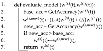
Algorithm 1, termed Sequential Aggregation (SA), describes how a server incrementally incorporates peer model updates in a time step . In this algorithm, the server evaluates the baseline accuracy of its model using the function GetAccuracy (line 2). Then, it computes a candidate-updated model using (2) (line 3). The candidate model’s accuracy is evaluated (line 4); if the new accuracy exceeds the baseline, the server adopts the candidate update; otherwise, it retains its current model (lines 5–7). This process is repeated sequentially for models from different peer servers.
| Algorithm 1: Sequential Aggregation (SA) |
| Input: server model , peer server model (, aggregation parameter ( Output: updated server model |
 |
When a server receives multiple updates at once, it applies them in ascending order of . Starting with low- updates ensures that models trained on smaller samples can still contribute; if high- updates (those based on larger datasets) are applied first, subsequent low- updates may no longer improve the model.
- Binary Aggregation (BA)
In the Binary Aggregation approach, each server first evaluates both its own model and the models received from peer servers using its validation dataset. The evaluation metric (e.g., accuracy) is computed for each model using (1), and the model achieving the highest performance is selected. This best-performing model is then disseminated to the server’s clients for local training. This approach ensures that each server adopts the model that demonstrates the best performance on its validation set at each training round.
- Dynamic Weighted Averaging Aggregation (DWAA)
In Dynamic Weighted Averaging Aggregation, similar to SA and BA, each server first evaluates its own model and the models received from peer servers using its validation dataset. For each model, the server computes the accuracy by comparing the model’s predictions with the true labels in the validation dataset. These accuracy values are then normalized to compute weights for each model, as follows:
where is the accuracy of model . These weights reflect the relative performance of each model on the validation dataset. The server then updates its model as a weighted linear combination of all models, with each model weighted according to its respective accuracy using (5).
This method ensures that models with higher accuracy on the validation dataset contribute more to the server model, while lower-performing models have less influence. By dynamically adjusting the contribution of each model, this approach aims to optimize the aggregation process and improve the overall model performance.
- Statistical Performance-Aware Aggregation (SPAA)
In this method, each server evaluates both its own model and the models received from peer servers, using a Negative Log Likelihood Loss (NLLLoss) performance metric. The NLLLoss is calculated over the validation dataset available at each server and serves as the key criterion for assessing model performance. This approach prioritizes models that produce high-confidence predictions for the correct classes, resulting in lower loss values . For each batch of validation data, the NLLLoss is computed and accumulated to track the overall loss across the entire validation dataset. The total loss is then normalized by the number of samples to calculate the average validation loss for each model. The average validation loss is used to determine how much each model contributes to the final aggregated model at each server. Models with lower validation loss are assigned higher weights in the aggregation process, while those with higher validation loss are penalized using statistical weighting. This penalization helps to minimize the impact of poorly performing models in the aggregation process.
At each server, the validation losses are analyzed statistically to identify underperforming models. The proposed method leverages the -score, a standardized metric that quantifies how far a particular value deviates from the mean, thus effectively capturing each value’s outlier strength. To begin, we compute the mean and standard deviation of all validation losses:
where is the number of models being considered. Each model’s loss is converted into a -score to quantify how much it deviates from the mean loss. Models whose exceeds a selected threshold (e.g., ) are deemed outliers and are penalized to reduce their impact on the final aggregated model. The penalty for each model is computed using a sigmoid function as follows:
where is the penalty for the server s model, which decreases the contribution of models with higher deviations from the mean loss. Once the penalties are applied, the adjusted weights for each model are computed as follows:
The weights are normalized using (10) to ensure that they sum to one. Each server aggregates the models using a weighted sum of their parameters, where models with lower validation loss contribute to the final aggregated model.
This approach ensures that models with significant deviations are penalized, contributing less to the aggregated global model.
In the proposed aggregation models, we primarily utilized accuracy and loss as performance metrics. However, other performance indicators can be incorporated to assess models’ effectiveness and adjust their contribution based on specific performance objectives and system requirements, ensuring adaptability in various application scenarios.
Algorithm 2 details how each FL server in the proposed MS-FL framework—with DWAA and SPAA mechanisms—handles both inter-server collaboration and vehicles’ models’ aggregation at each communication round . Initially, if no pre-trained model exists, the server randomizes its model weights (Line 1). At the beginning of round , the server collects models from its peer servers (Line 3) and evaluates their performance on its validation dataset (Line 4) using accuracy and loss metrics. Then the server normalizes these performance metrics—applying z-score penalties for SPAA—and computes the contribution weights (Line 5). The server then merges the peer models into its current model via a weighted sum (Line 6). Following the server-level aggregation, the server selects clients using a client selection algorithm, (Line 7), and distributes its current model to the chosen vehicles (Line 8). This process repeats until the training rounds reach a preset limit or the server’s model achieves the desired accuracy.
| Algorithm 2: FL server operation in MS-FL using SPAA/DWAA |
| Input: servers’ models (, vehicles’ models (). Output: updated server model |
| #Initialize the model at server |
 |
Table 2 summarizes the key strengths and limitations of each proposed aggregation method.
Table 2.
Comparative summary of aggregation strategies in MS-FL, highlighting each method’s core mechanism, key advantages, and potential limitations.
4.2. Intra-Server Training Phase
4.2.1. Local Training on Vehicles
Every selected vehicle initiates local training on its own dataset for epochs using iterative optimization methods, such as Stochastic Gradient Descent (SGD) [5,6]. During local training, the vehicle’s dataset is partitioned into batches of data points. For each batch, the local model parameters are updated using (11) [5]:
where is the learning rate and is the average gradient computed on vehicle ’s local dataset with respect to the server model . The updated model reflects the improvements made during local training.
4.2.2. Vehicles’ Models’ Aggregation at Server
For simplicity, we assume that the Federated Averaging (FedAvg) [5,6] algorithm is employed at each server to efficiently merge local updates from vehicles; however, other client aggregation approaches would work as well. Once local training is finished, each client sends its updated model to its associated server. The server aggregates these updates through FedAvg, a weighted average that factors in each client’s proportion of the total training data [5]. This process produces an updated server model , which is then distributed back to the clients for the next training round.
In the proposed MS-FL, each server collects both server model updates from its peer servers, and local model updates from vehicles within its coverage area, and uses these updates to refine models. A key element of this process is a model aggregation algorithm that consolidates parameters from different servers to form a comprehensive server model.
In the intra-server training phase, each server enforces a round deadline . At , it aggregates whatever subset of updates has been received; late arrivals are discarded for that round.
During the inter-server phase, models forwarded by server arrive at server after a deterministic backhaul delay . If , that update is applied in the next round.
4.3. Clients’ Movements and Handover
In cellular networks, as a user moves between cells during an ongoing session, a handover procedure must be performed to avoid any interruption in service [24,25,26]. In our FL setting, we face a similar challenge—but instead of radio-control signaling, we must migrate model updates between servers to keep a vehicle’s training continuous and prevent lost gradients.
Federated learning handovers differ fundamentally from traditional cellular handovers in both the data volume exchanged and the service objectives they must achieve. Whereas a cellular handover exchanges only small control and radio link-state messages—typically on the order of a few kilobytes [24], making transfer delay negligible—an FL handover must migrate the vehicle’s model updates, which can range from megabytes to gigabytes of weights or gradient deltas [2,27].
In our scenario, illustrated in Figure 2, vehicles traverse multiple server coverage zones. If a selected vehicle exits its assigned server’s range before uploading its locally trained model, that update is lost. To address this, we introduce an application layer handover that complements the standard cellular handover, ensuring uninterrupted training continuity and preserving model updates. Each migrating vehicle selects its new RSU by evaluating the cellular handover criteria—strongest signal, lowest latency and highest capacity—and then attaches to it. Upon attachment, the new server immediately broadcasts a concise message containing the domain tag (e.g., “traffic sign image classification”), the expected input format (e.g., image resolution, color vs. grayscale), and the model ID/version (to confirm classifier architecture and preprocessing). Then, the vehicle compares these requirements against its local model metadata; if they match, it packages its latest parameters and metadata and uploads them to the new server, which enqueues them into the aggregation pipeline so that the vehicle can resume participation or receive further training tasks. If the requirements do not match, the server rejects the update outright, preventing misaligned contributions from degrading the global model.
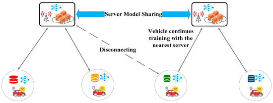
Figure 2.
MS-FL architecture considering mobility and handover.
When a vehicle that was selected by server moves into the coverage area of another server during the communication round , it continues its local training under . Let the following be carried out:
- be the set of vehicles that both started and completed their local updates entirely within server ’s coverage during round t;
- be the set of vehicles that began training under server but crossed into ’s coverage before uploading their update.
Each vehicle produces a locally trained model . Each vehicle produces a locally trained model , where that model was initialized from server ’s state some epochs earlier. At the end of round t, server aggregates the following:
Here, is the nonnegative weight that server assigns to vehicle k’s update. In particular, as follows:
where reflects vehicle k’s fraction of the total samples used in round t at server .
where is the number of training samples at client when it was served by server and is the set of all vehicles that completed training under server in round t. Intuitively, gives proportional weight to servers that host more data. If one sets for every server , then Equation (13) reduces to the standard FedAvg aggregation. Conversely, if for some servers , then none of s’s vehicles’ updates are included in ’s aggregation. In practice, a “crowded” server—i.e., one with more total training samples— receives a larger , thereby granting its updates greater influence on ’s new model.
By combining updates from vehicles that trained fully under and those that handover from any other , Equation (13) ensures that no completed local update is lost when a vehicle moves between coverage areas.
This application layer handover is independent of the link and physical layer handover, which are managed automatically by standardized cellular procedures. Once verified, the vehicle resumes participation by uploading its model updates or receiving further training tasks from the new server.
By integrating this handover mechanism, our framework minimizes update loss and maintains model integrity, even in highly dynamic vehicular environments.
5. Transmission Latency Analysis
In FL, transmission delays overwhelmingly dictate the overall runtime, rendering local computation times relatively insignificant [5,6]. Thanks to advances in Central Processing Unit (CPU) and Graphics Processing Unit (GPU) technologies, on-device training has become highly efficient, shifting the primary bottleneck to communication. Contemporary ML models often require hundreds of megabytes—and in some cases gigabytes—of parameters [2,28,29], and achieving convergence can demand on the order of hundreds of thousands of communication rounds. Consequently, the aggregate volume of exchanged updates can easily reach the petabyte scale over a full training cycle [27]. Unlike centralized training, FL performance is therefore constrained by its communication overhead—a constraint that becomes even more severe under poor network conditions. In the following section, we evaluate transmission latency across three architectures: our proposed MS-FL framework, a conventional single-server FL setup, and a cloud-based FL system.
5.1. MS-FL
In our MS-FL framework, the total transmission latency in each communication round denoted by comprises three key components: the local uploading time from clients to their regional FL servers, the downloading time from regional servers to clients, and the inter-server (RSU-to-RSU) transmission time. Owing to the significantly higher communication capabilities of RSU-to-RSU links compared to client-to-RSU links, the overall latency is predominantly determined by the maximum latency among the clients. Nonetheless, the inter-server latency is also accounted for in the analysis.
- Client-to-RSU Communication: For each client in round , the uploading time to its associated server is given by the following:
As in [18,19], we use Shannon’s formula [30] to model the uplink rate under noise-limited conditions. The uplink rate is given by the following:
where represents the uplink transmit power and denotes the uplink channel gain at time t. The noise power is .
Similarly, the downloading time from server to client is modeled as follows:
where is the size (in bits) of the data that client downloads from server , is the downlink bandwidth allocated by server s to client , and is the achievable downlink rate (in bits/s/Hz) from server s to client i at round t, given by the following:
where is the downlink transmit power and is the downlink channel gain at time t.
- RSU-to-RSU Communication: Although RSUs typically use high-speed backhaul links [31], we include the following general mode for completeness. The latency to exchange a model between two servers at round t is as follows:
- Overall Transmission Latency: Assuming that training must proceed for rounds to reach the target performance, the total transmission latency is simply the sum of the per-round latencies:
Here, is the slowest client upload time at round t. is the slowest client download time at round t. And is the longest RSU-to-RSU transfer time in that round. Since RSU–RSU delays are negligible, the dominant component is the “edge” delay—the sum of the slowest client upload and download times:
5.2. Single-Server FL
In a single-server FL architecture, each client sends its model updates via its local RSU, which then forwards them over the high-speed backhaul to the central server. Because RSU–RSU (backhaul) delays are negligible, the per-round transmission latency reduces to the same “edge” delay defined in the MS-FL subsection—that is, the slowest client’s upload plus download time. If clients were to communicate directly with the central server, increased path loss and lower spectral efficiency over longer distances would substantially raise latency [32,33]. Although various algorithms have been proposed to accelerate convergence in single-server FL [33,34,35], the overall transmission time remains dominated by this edge delay summed over all communication rounds.
5.3. Cloud-Based FL
Hierarchical cloud-based FL [10] architectures incorporate both edge servers and a cloud server, operating two distinct aggregation processes: edge aggregation and global aggregation.
- Edge aggregation: Exactly as in MS-FL and single-server FL, clients exchange updates with their local server. The per-round “edge” delay is therefore the same defined in Section 5.1.
- Global aggregation: After edge aggregation, the cloud server aggregates the models from the various edge servers. The transmission latency for global aggregation is expressed as follows:
Here, and denote the uplink and downlink latencies from edge server to the cloud server in round , respectively.
- Overall Transmission Latency: The end-to-end transmission time to achieve the targeted accuracy is the sum of the latencies over all edge and global aggregation rounds. Assuming the two layer federated learning process requires global aggregation rounds to reach the specified performance level, the total transmission latency is given by the following:
It is important to note that the RSU-to-cloud (global) transmissions typically incur higher latencies due to the longer distances between regional servers and the cloud compared to those between clients and regional servers. Consequently, . This increased latency contributes to a longer overall convergence time for cloud-based FL compared to single-server FL or MS-FL architectures.
In summary, while cloud-based FL enhances scalability and allows for more efficient local aggregation, its overall communication delay is higher due to the additional global aggregation phase and the larger transmission distances involved. This trade-off must be considered when designing FL systems in large-scale networks.
5.4. Handover Latency
As noted in Section 5.1, each round’s latency is driven by the slowest client’s upload + download time ( in (24)). Since that term already captures the worst-case edge delay, we only need to check whether handovers add any extra latency.
Under a standard LTE/5G conditional handover—where Radio Resource Control (RRC) commands are pre-installed and the User Equipment (UE) automatically executes them once a neighbor’s Reference Signal Received Power (RSRP) exceeds the serving RSRP via configured hysteresis for the Time-to-Trigger [24,36]—all control-plane signaling (handover request, verify, ACK, and RRC handover command) is effectively instantaneous, and its latency is negligible in comparison to moving the model update itself. In a symmetric setup (where each RSU allocates equal uplink bandwidth to all its clients), a migrating vehicle simply resumes its upload under the same bandwidth allocation. Therefore, the handover upload delay remains bounded by the usual edge delay , and application-level handovers do not introduce any significant amount of additional delay.
6. Experimental Results
6.1. Simulation Setup
Various simulations were conducted on a GPU server equipped with an NVIDIA A100-PCIE-40GB GPU, running Ubuntu 24.04 LTS (GNU/Linux 6.8.0-36-generic x86_64). The environment was configured with CUDA version 12.2 and PyTorch version 2.3.1 [37]. Our FL framework extends the PyTorch FL implementation provided in [38]. The results were averaged over multiple independent trials using a Convolutional Neural Network (CNN) architecture.
Our experiment employed a CNN due to its superior ability to extract spatial features from image data and its proven effectiveness in image classification tasks. The model consists of two convolutional layers, with the first layer containing 32 channels and the second layer comprising 64 channels, both followed by max pooling layers. Additionally, the network includes a fully connected layer with 512 units and ReLU activation, concluding with a softmax output layer. The entire model contains 1,663,370 parameters.
6.2. Dataset
We evaluated our framework on two standard image-classification benchmarks (Figure 3):
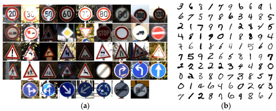
Figure 3.
Sample images from the benchmarks: (a) one example per class from the 43 traffic sign categories in GTSRB [39]; (b) handwritten digits from MNIST [40].
- GTSRB [39] provides 26,640 RGB traffic sign images for training and 12,630 for testing, across 43 classes. Sample images are shown in Figure 3a.
- MNIST [40] contains 60,000 grayscale training images and 10,000 test images of handwritten digits (28 × 28 px, 10 classes). Sample images are shown in Figure 3b.
For each dataset, we first resized all images to 32 × 32 px, then split the original training set into 80% training and 20% validation. This split is stratified by class label: the proportion of examples from each digit or sign category is maintained in the training and validation pools. As a result, every class remains well represented in the validation data that each server uses to assess incoming peer models. This balanced, stratified division guards against evaluation bias—where rare classes might otherwise be under or over-sampled—and provides an accurate measure of each model’s generalization before it contributes to the global aggregation.
6.3. Comparision Schemes
To highlight the advantages of the proposed MS-FL architecture, we benchmark it against two representative baselines:
- Cloud-based FL (hierarchical FL)—following the layered design in [10], edge servers serve as intermediaries between vehicles and a single cloud server. Each client trains locally for epochs and uploads its parameters to its server; the server aggregates these updates, then forwards the result to the cloud. The cloud performs a second-level aggregation across all servers and broadcasts the global model back. Crucially, servers cooperate only through the cloud—no peer-to-peer exchange occurs;
- Isolated single-server FL at each RSU—here, every RSU acts as an independent FL server [5,6]. It trains a model using only the clients in its own coverage area and never exchanges parameters with either peer servers or a cloud node. This baseline captures the performance of a non-collaborative multi-server deployment.
By comparing MS-FL against these two schemes—one that centralizes coordination at the cloud and one that eliminates inter-server collaboration entirely—we can clearly quantify the benefits of direct, cooperative aggregation among servers in our proposed framework.
6.4. Simulation Results
In our experiments, we deployed three FL servers (), each at a distinct RSU, and evaluated two scenarios: a shard-based dataset distribution with 48 clients in total, and a Dirichlet-based distribution with 100 clients in total. The clients were evenly distributed among the servers, with each server responsible for approximately one-third of the clients.
To quantify the recognition quality for the proposed MS-FL framework, we record, for every class, the four canonical outcomes of a classifier:
- True positives (TP)—images that truly belong to a class and are labeled as such by the model (e.g., a “speed-limit-30 km h” sign or a handwritten ‘8’ identified correctly);
- True negatives (TN)—images that do not belong to the class and are correctly rejected;
- False positives (FP)—images that are erroneously assigned to the class (a “speed-limit-50” labeled as “30”; a ‘3’ labeled as ‘8’);
- False negatives (FN)—images that should have been assigned to the class but were missed by the model.
From these counts, we report three widely accepted indicators:
- Precision—the proportion of predicted positives that are indeed correct. High precision shows that the model rarely confuses one traffic sign (or digit) for another;
- Recall—the proportion of actual positives retrieved by the model. A high recall means that very few relevant signs or digits are overlooked;
- F1-score—the harmonic balance between precision and recall, providing a single, robust measure of overall classification effectiveness.
6.4.1. Performance Evaluation of the Proposed Server-Level Aggregation Methods
To benchmark our proposed MS-FL framework against the vanilla FL setup [5]—which does not share knowledge between servers—we adopted the same shard-based non-IID distribution from [5]. Specifically, we sorted the dataset by class label (43 categories), divided it into 96 shards of 222 samples each, and assigned two shards to each of the 48 clients. We then ran 500 training rounds and reported training loss, training accuracy, test accuracy, F1-score, precision, and recall for our MS-FL aggregation methods. For comparison, we include the results for the baseline FL model without any server-level evaluation or aggregation—referred to as the “Without Aggregation” (WA) model.
Table 3 summarizes the performance metrics, average test recall, test accuracy, test precision, and test F1-score for the proposed aggregation methods and vanilla FL in a multi-server FL framework with three servers. The results, averaged across the servers after 500 training rounds, indicate that SPAA outperforms all other methods across all evaluation metrics, achieving the highest test recall (75%), test accuracy (84%), precision (78%), and F1-score (76%). This performance underscores the effectiveness of SPAA’s statistical weighting and aggregation technique in enhancing model performance. DWAA and SA also deliver strong results, surpassing BA and significantly outperforming WA in all metrics, highlighting the benefits of performance-based aggregation methods. Although SPAA, DWAA, and SA exhibit slightly higher runtimes than WA due to additional evaluation and aggregation steps, the substantial gains in accuracy and recall justify the increased computational cost, making SPAA a highly effective method for MS-FL in environments with data heterogeneity.
Table 3.
Performance evaluation on GTSRB dataset after 500 training rounds for MS-FL.
Figure 4 presents comparisons of training accuracy and training loss, between the proposed aggregation methods and vanilla FL [4] over 500 training rounds. The results are averaged across three servers for each method, providing a comprehensive view of model performance in an FL setting. The proposed methods, particularly SPAA and DWAA, demonstrate improved training accuracy compared to vanilla FL (i.e., WA). Additionally, SPAA, DWAA, and SA exhibit better results in terms of training loss compared to vanilla FL.
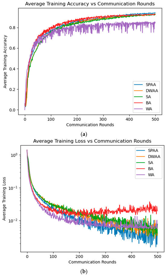
Figure 4.
MS-FL training on GTSRB dataset (shard-based non-IID) over 500 rounds with a CNN: (a) average training accuracy; (b) average training loss (log scale on the y-axis).
To isolate SPAA’s contribution, we disable its z-score penalty—setting every penalty to 1—so that SPAA reverts to a loss-weighted DWAA where weights are proportional to raw loss values. We then compare the average test accuracy curves to reveal the impact of the statistical penalty. As Figure 5 shows, SPAA with the z-score penalty delivers slightly higher accuracy at both 50 and 200 rounds—particularly in the early phases—indicating faster convergence. While the absolute difference is modest in our benign setting, we expect the penalty to provide substantially larger benefits under adversarial or high-noise conditions.
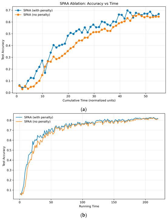
Figure 5.
Ablation of SPAA’s outlier penalty on the GTSRB dataset (Dirichlet split, ). Test accuracy versus normalized time units (one unit = one communication round), averaged across three RSUs: (a) over 50 rounds, (b) over 200 rounds.
6.4.2. Comparative Experiments: MS-FL vs. Baselines
To evaluate and compare three FL architectures—single-server FL, cloud-based FL, and our proposed MS-FL—we distributed each client’s data by sampling class proportions from a Dirichlet distribution (concentration parameter ) and assigning images accordingly. Figure 6 shows the average test accuracy on MNIST after 5, 10, and 15 communication rounds. Across all rounds, MS-FL consistently outperforms single-server FL, and closely tracks cloud-based FL. While cloud-based FL retains a small accuracy lead—~93% vs. ~91% at 15 rounds—MS-FL avoids the additional communication with the cloud server for every training round, thereby saving communication bandwidth and reducing transmission latency.
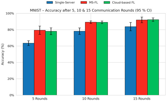
Figure 6.
Average test accuracy (%) on the MNIST dataset (non-IID split with Dirichlet α = 0.1) after 5, 10, and 15 communication rounds under three FL frameworks—single-server FL, the proposed MS-FL with DWAA, and cloud-based FL. Error bars denote the 95% confidence interval across five independent runs.
Figure 7 shows test accuracy, precision, recall and F1-score for the three FL frameworks after five and ten communication rounds (five runs, 95% CI). At both checkpoints, MS-FL dramatically outperforms the single-server baseline—improving every metric by roughly twenty percentage points—and matches the performance of cloud-based FL within its confidence intervals. The gap between MS-FL and cloud-based FL is consistently small (around one to three percentage points), demonstrating that MS-FL achieves near-cloud accuracy while avoiding per-round global aggregation.
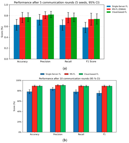
Figure 7.
Performance comparison of three FL frameworks—single-server FL, proposed MS-FL with DWAA, and cloud-based FL—on MNIST with a Dirichlet non-IID split ( = 0.1). Bars denote the mean accuracy, precision, recall, and F1-score after (a) 5 communication rounds and (b) 10 rounds (averaged over five runs).
Table 4 reports the average performance of the three FL frameworks on the GTSRB dataset (Dirichlet non-IID split, α = 0.1) using a CNN model after 50 communication rounds. Each value is averaged over the three servers. Our MS-FL framework with DWAA achieves the highest accuracy (73.29%), precision (62.32%), recall (62.26%), and F1-score (60.45%), compared to cloud-based FL and single-server FL.
Table 4.
Performance evaluation on GTSRB dataset (non-IID split via Dirichlet, = 0.1) with a CNN model after 50 communication rounds.
Figure 8 extends this comparison to 200 communication rounds, averaged over 30 independent runs (95% CI). After 200 rounds, cloud-based FL marginally outperforms MS-FL in all four metrics, but it incurs significantly higher transmission latency (as shown in Figure 7). In contrast, MS-FL with DWAA converges faster, achieving near-peak performance well before 200 rounds.
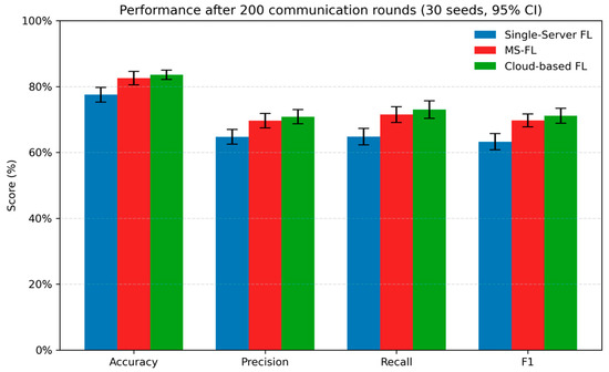
Figure 8.
Performance comparison of three FL frameworks on GTSRB with a Dirichlet non-IID split ( = 0.1). Bars denote the mean accuracy, precision, recall, and F1-score after 200 communication rounds (averaged over 30 independent runs). Error bars indicate 95% confidence intervals.
6.4.3. Convergence Speed Under Latency Constraints
We adopt the normalization from [41] by fixing the ratio of edge communication to the local computation time at 10 and then setting the normalized edge round cost to 1. Similarly to [18], we use the cloud to edge latency ratio as , which is greater than 1 because client–edge–cloud communication in hierarchical FL is substantially slower than client–edge communication. Consistent with [10,41], we use and for cloud-based FL.
Concretely, we model each edge server round as 1 ms of wireless transmission plus 0.1 ms of local computation (so 1.1 ms per round) for both MS-FL and single-server FL. For the cloud-based hierarchy scheme, we use a 5 ms and 10 ms end-to-end client–cloud latency plus 0.1 ms of computation, yielding 5.5 ms and 10.5 ms per round. These settings—drawn from [10,18,19,41]—allow us to compare convergence speed under realistic network and processing delays.
Figure 9 compares test accuracy over cumulative running time for three FL schemes on both MNIST and GTSRB. In both plots, the DWAA-based MS-FL (orange curve) achieves near-final accuracy in far fewer time units than the other methods. On MNIST (Figure 7a), DWAA reaches over 90% accuracy within roughly 10 ms, whereas single-server FL (blue) needs about 30 ms and the two cloud-based variants (green and red) lag behind. On the more challenging GTSRB dataset (Figure 7b), the same ordering holds: DWAA converges most rapidly, single-server FL follows, and cloud-synchronized FL suffers the greatest delay.
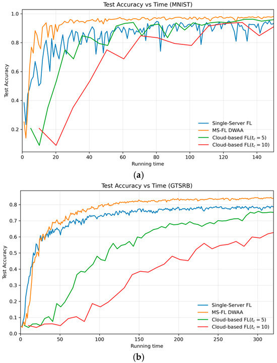
Figure 9.
Test accuracy vs. normalized running time for single-server FL, MS-FL (DWAA), and cloud-based FL with and , on (a) MNIST and (b) GTSRB.
6.4.4. Mobility and Handover Effects
Figure 10 shows the average test accuracy of single-server FL, cloud-based FL, and MS-FL (DWAA) under three mobility scenarios: none, dropout, and handover. In the none scenario—where all vehicles stay within their original server’s coverage—single-server FL achieves 76% accuracy, cloud-based FL 88%, and MS-FL 87%. Introducing a 40% dropout, in which randomly selected vehicles fail to upload their updates, reduces accuracy to 61% for single-server FL, 85% for cloud-based FL, and 83% for MS-FL. When handover is enabled, so that migrating vehicles can successfully transfer their models, accuracy rebounds to 81% for single-server FL and to 91% for both cloud-based FL and MS-FL.
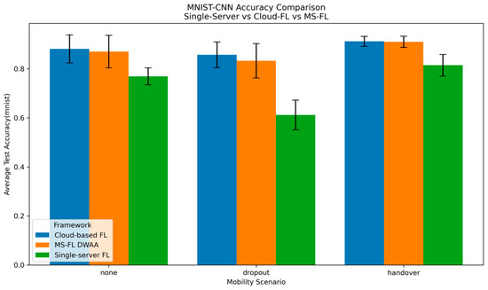
Figure 10.
Average test accuracy under a Dirichlet (α = 0.1) non-IID split, comparing single-server FL, cloud-based FL, and MS-FL (DWAA) across three mobility scenarios—none, dropout, and handover after 10 communication rounds.
Notably, the 95% confidence intervals for cloud-based FL (0.8915–0.9321 under handover vs. 0.8239–0.9382 under none) and MS-FL (0.8875–0.9328 vs. 0.8039–0.9372) overlap almost completely, indicating that both frameworks perform equivalently in the none and handover scenarios. Single-server FL benefits from handover—its CI-high rises from 80% in the none scenario to 85% under handover—because handover enables indirect model sharing across RSUs, which does not occur when vehicles remain within one RSU’s coverage throughout the training process. These additional cross-server updates allow the global model to learn more quickly from diverse client data, producing the accuracy gain.
Figure 11 plots the test accuracy and loss versus normalized running time on the MNIST dataset for each FL framework under three conditions: none, dropout, and handover. In the none scenario (solid lines), MS-FL with SPAA achieves the highest accuracy and lowest loss, converging in just 20 rounds. In the dropout scenario (40% drop rate), because only 10% of clients participate each round—and those clients are evenly distributed across three RSUs—a 40% dropout corresponds to losing just one client’s update per server. As a result, all frameworks experience some performance degradation, but MS-FL with SPAA still converges by round 20 to nearly the same accuracy and loss levels, demonstrating resilience to occasional missing updates. When handover is enabled—so migrating vehicles can successfully upload their models to the new RSU—both MS-FL and cloud-based FL recover performance close to the none baseline. Interestingly, single-server FL also benefits under handover: indirect model exchanges among RSUs improve its convergence compared to the none case, where no inter-server interaction occurs.
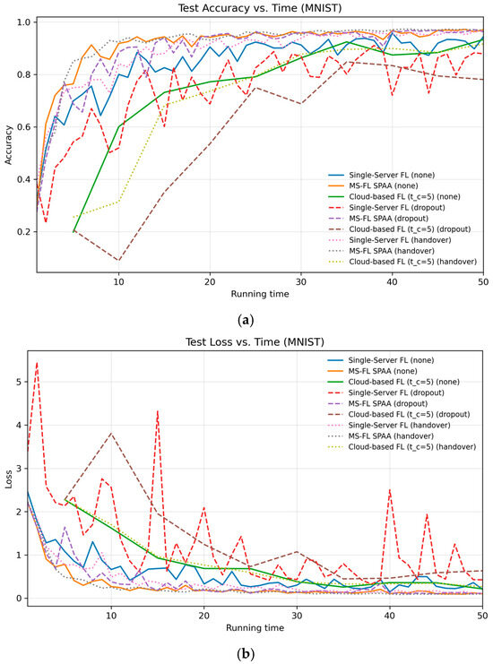
Figure 11.
Test performance on MNIST versus normalized running time, comparing single-server FL, MS-FL (DWAA), and cloud-based FL () under three conditions—none, dropout, and handover. (a) Accuracy over time, (b) loss over time.
Figure 12 plots the test accuracy versus normalized running time on GTSRB (we set the cloud round latency factor to , with edge server latency = 1 unit and computation = 0.1, as detailed in Section 6.4.3). Here, both single-server FL and MS-FL DWAA (plotted for dropout and handover) converge much more quickly than cloud-based FL: the cloud-based curves start at a larger time offset (reflecting the edge–cloud round delay) and take significantly longer to plateau. In contrast, MS-FL DWAA achieves around 0.80 accuracy by and nearly 0.85 by , whereas single-server FL lags behind. Enabling handover (dashed lines) further boosts accuracy, most notably for single-server FL, demonstrating that preserving and forwarding “lost” updates can meaningfully mitigate the effects of client mobility.
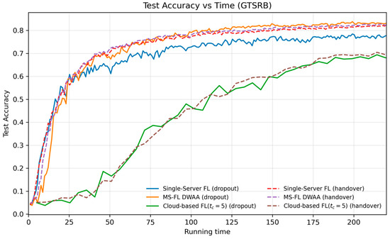
Figure 12.
Test accuracy versus normalized running time on the GTSRB dataset, comparing single-server FL, MS-FL (DWAA), and cloud-based FL () under dropout (solid lines) and handover (dashed lines) scenarios.
7. Discussion and Future Directions
To enhance privacy in autonomous vehicle machine learning, this paper proposed a novel MS-FL framework designed specifically for the data heterogeneity and mobility of autonomous vehicle networks. By enabling neighboring servers to exchange model updates directly—rather than routing everything through a central cloud—MS-FL achieves faster convergence and superior predictive performance compared to both single-server FL and hierarchical edge cloud-based FL. Crucially, MS-FL edges out the cloud-based approach without requiring any RSU–cloud communication, slashing end-to-end latency and conserving backbone bandwidth.
Our MS-FL framework overcomes the limitations of prior edge-only and cloud-based schemes through two core innovations. First, at the server level, each server evaluates peer models on its own validation data and aggregates them using performance-driven strategies (BA, SA, DWAA, and SPAA), ensuring that only high-quality contributions shape the global model and avoiding blind averaging under non-IID data. Second, MS-FL enables seamless handover with lost update preservation: when vehicles migrate between coverage areas, their local updates are retained and forwarded to the next server, preventing wasted training effort and maintaining the continuity of learning. By sharing and weighting these high-quality updates from diverse locations—filtering out outliers and stale models before they can degrade performance—MS-FL accelerates convergence in highly heterogeneous vehicular environments.
Under a “dropout” failure scenario—where migrating vehicles fail to upload their updates—enabling handover speeds up convergence in MS-FL, particularly during the early communication rounds. Introducing handover into single-server FL produces even larger relative gains, as it facilitates the indirect exchange of model updates among servers and significantly improves its convergence speed.
Across both shard-based and Dirichlet-based non-IID data splits—and under both dropout and handover mobility scenarios—MS-FL consistently delivers superior accuracy, precision, recall, and F1-scores compared to vanilla FL. SPAA, in particular, shines by dynamically weighting updates according to their statistical reliability, while DWAA and SA also significantly outperform the baseline, demonstrating that even simple performance-based filtering can yield substantial gains.
For future work, we will extend our evaluation to real-world mobility scenarios, using driving simulators to measure end-to-end performance under dynamic RSU handovers, variable link latency, and evolving data streams. We will also assess MS-FL’s resilience to adversarial threats—such as model poisoning and inference attacks—and develop incentive mechanisms to ensure sustained client participation, which is essential for fairness and scalability in federated settings. Finally, incorporating privacy-preserving techniques like differential privacy or secure aggregation will further safeguard user data, laying the groundwork for efficient, secure, and scalable FL in next-generation connected vehicles.
Author Contributions
Conceptualization, S.S.H. and K.E.-K.; methodology, F.M., S.S.H. and K.E.-K.; software, F.M.; validation, F.M., S.S.H. and K.E.-K.; formal analysis, F.M.; investigation, F.M.; resources, S.S.H. and K.E.-K.; data curation, F.M.; writing—original draft preparation, F.M.; writing—review and editing, F.M., S.S.H. and K.E.-K.; visualization, F.M.; supervision, S.S.H. and K.E.-K.; project administration, S.S.H.; funding acquisition, S.S.H. and K.E.-K. All authors have read and agreed to the published version of the manuscript.
Funding
NSERC Grant RGPIN/004408-2019.
Data Availability Statement
The original contributions presented in this study are included in the article. Further inquiries can be directed to the corresponding author.
Conflicts of Interest
The authors declare no conflict of interest.
References
- Grigorescu, S.; Trasnea, B.; Cocias, T.; Macesanu, G. A survey of deep learning techniques for autonomous driving. J. Field Robot. 2020, 37, 362–386. [Google Scholar] [CrossRef]
- Brown, T.B.; Mann, B.; Ryder, N.; Subbiah, M.; Kaplan, J.; Dhariwal, P.; Neelakantan, A.; Shyam, P.; Sastry, G.; Askell, A.; et al. Language models are few-shot learners. arXiv 2020, arXiv:2005.14165. [Google Scholar] [CrossRef]
- Lu, Y.; Huang, X.; Zhang, K.; Maharjan, S.; Zhang, Y. Blockchain empowered asynchronous federated learning for secure data sharing in Internet of Vehicles. IEEE Trans. Veh. Technol. 2020, 69, 4298–4311. [Google Scholar] [CrossRef]
- Häfner, B.; Jiru, J.; Schepker, H.; Schmitt, G.A.; Ott, J. Proposing cooperative maneuvers among automated vehicles using machine learning. In Proceedings of the 24th International ACM Conference on Modeling, Analysis and Simulation of Wireless and Mobile Systems (MSWiM ’21), Alicante, Spain, 22–26 November 2021; Association for Computing Machinery: New York, NY, USA, 2021; pp. 173–180. [Google Scholar]
- McMahan, B.; Moore, E.; Ramage, D.; Hampson, S.; y Arcas, B.A. Communication-efficient learning of deep networks from decentralized data. In Proceedings of the 20th International Conference on Artificial Intelligence and Statistics (AISTATS), Fort Lauderdale, FL, USA, 20–22 March 2017; pp. 1273–1282. [Google Scholar]
- Kairouz, P.; McMahan, H.B.; Avent, B.; Bellet, A.; Bennis, M.; Bhagoji, A.N.; Bonawit, K.; Charles, Z.; Cormode, G.; Cummings, R.; et al. Advances and Open Problems in Federated Learning. arXiv 2021, arXiv:1912.04977. [Google Scholar] [CrossRef]
- Moon, S.; Lim, Y. Client selection for federated learning in vehicular edge computing: A deep reinforcement learning approach. IEEE Access, 2024; in press. [Google Scholar]
- Cha, N.; Chang, L. Multi-objective distributed client selection in federated learning-assisted Internet of Vehicles. Sensors 2024, 24, 4180. [Google Scholar] [CrossRef] [PubMed]
- Albelaihi, R. Mobility prediction and resource-aware client selection for federated learning in IoT. Future Internet 2025, 17, 3. [Google Scholar] [CrossRef]
- Zhou, X.; Liang, W.; She, J.; Yan, Z.; Wang, K.I.-K. Two-layer federated learning with heterogeneous model aggregation for 6G supported Internet of Vehicles. IEEE Trans. Veh. Technol. 2021, 70, 5308–5317. [Google Scholar] [CrossRef]
- Lim, W.Y.B.; Luong, N.C.; Hoang, D.T.; Jiao, Y.; Liang, Y.-C.; Yang, Q.; Niyato, D.; Miao, C. Federated learning in mobile edge networks: A comprehensive survey. IEEE Commun. Surv. Tutor. 2020, 22, 2031–2063. [Google Scholar] [CrossRef]
- Liu, L.; Zhang, J.; Song, S.; Letaief, K.B. Client-edge-cloud hierarchical federated learning. In Proceedings of the IEEE International Conference on Communications (ICC), Dublin, Ireland, 7–11 June 2020; pp. 1–6. [Google Scholar]
- Wang, J.; Wang, S.; Chen, R.-R.; Ji, M. Local averaging helps: Hierarchical federated learning and convergence analysis. arXiv 2020, arXiv:2010.12998. [Google Scholar]
- Xie, M.; Long, G.; Shen, T.; Zhou, T.; Wang, X.; Jiang, J. Multicenter federated learning. arXiv 2020, arXiv:2005.01026. [Google Scholar]
- Lee, J.-W.; Oh, J.; Lim, S.; Yun, S.-Y.; Lee, J.-G. Tornadoaggregate: Accurate and scalable federated learning via the ring-based architecture. arXiv 2020, arXiv:2012.03214. [Google Scholar]
- Duan, M.; Liu, D.; Chen, X.; Liu, R.; Tan, Y.; Liang, L. Self-balancing federated learning with global imbalanced data in mobile systems. IEEE Trans. Parallel Distrib. Syst. 2020, 32, 59–71. [Google Scholar] [CrossRef]
- Taïk, A.; Mlika, Z.; Cherkaoui, S. Clustered vehicular federated learning: Process and optimization. IEEE Trans. Intell. Transp. Syst. 2022, 23, 25371–25383. [Google Scholar] [CrossRef]
- Han, D.-J.; Choi, M.; Park, J.; Moon, J. FedMes: Speeding up federated learning with multiple edge servers. IEEE J. Sel. Areas Commun. 2021, 39, 3870–3885. [Google Scholar] [CrossRef]
- Qu, Z.; Li, X.; Xu, J.; Tang, B.; Lu, Z.; Liu, Y. On the convergence of multi-server federated learning with overlapping area. IEEE Trans. Mob. Comput. 2023, 22, 6647–6662. [Google Scholar] [CrossRef]
- Rjoub, G.; Wahab, O.A.; Bentahar, J.; Bataineh, A. Trust-driven reinforcement selection strategy for federated learning on IoT devices. Computing, 2022; in press. [Google Scholar]
- Mazloomi, F.; Shah Heydari, S.; El-Khatib, K. Trust-based knowledge sharing among federated learning servers in vehicular edge computing. In Proceedings of the International ACM Symposium on Design and Analysis of Intelligent Vehicular Networks and Applications, Montreal, QC, Canada, 30 October–3 November 2023; Association for Computing Machinery: New York, NY, USA, 2023; pp. 9–15. [Google Scholar]
- Liu, L.; Chen, C.; Pei, Q.; Maharjan, S.; Zhang, Y. Vehicular edge computing and networking: A survey. arXiv 2019, arXiv:1908.06849. [Google Scholar] [CrossRef]
- Liu, S.; Yu, J.; Deng, X.; Wan, S. FedCPF: An efficient-communication federated learning approach for vehicular edge computing in 6G communication networks. IEEE Trans. Intell. Transp. Syst. 2021, 23, 1616–1629. [Google Scholar] [CrossRef]
- 3GPP. Evolved Universal Terrestrial Radio Access (E-UTRA); Radio Resource Control (RRC); Protocol Specification (Release 16), 3GPP TS 36.331 V16.5.0; 3GPP: Sophia Antipolis, France, 2021; Available online: https://www.3gpp.org/ftp/Specs/archive/36_series/36.331/ (accessed on 15 May 2025).
- Han, J.; Wu, B. Handover in the 3GPP Long Term Evolution (LTE) systems. In Proceedings of the 2010 Global Mobile Congress (GMC), Shanghai, China, 18–19 October 2010; IEEE: Piscataway, NJ, USA, 2010; pp. 1–6. [Google Scholar]
- Ekiz, N.; Salih, T.; Küçüköner, S.; Fidanboylu, K. An overview of handoff techniques in cellular networks. Database 2005, 318, 6069. [Google Scholar]
- Zhou, Y.; Ye, Q.; Lv, J. Communication-efficient federated learning with compensated Overlap-FedAvg. IEEE Trans. Parallel Distrib. Syst. 2022, 33, 192–205. [Google Scholar] [CrossRef]
- Huang, G.; Liu, Z.; Van Der Maaten, L.; Weinberger, K.Q. Densely connected convolutional networks. In Proceedings of the IEEE Conference on Computer Vision and Pattern Recognition (CVPR), Honolulu, HI, USA, 21–26 July 2017; pp. 4700–4708. [Google Scholar]
- Xie, S.; Girshick, R.; Dollar, P.; Tu, Z.; He, K. Aggregated residual transformations for deep neural networks. In Proceedings of the IEEE Conference on Computer Vision and Pattern Recognition (CVPR), Honolulu, HI, USA, 21–26 July 2017; pp. 1492–1500. [Google Scholar]
- Shannon, C.E. A mathematical theory of communication. Bell Syst. Tech. J. 1948, 27, 379–423. [Google Scholar] [CrossRef]
- Vieira, E.; Almeida, J.; Ferreira, J.; Dias, T.; Vieira Silva, A.; Moura, L. A roadside and cloud-based vehicular communications framework for the provision of C-ITS services. Information 2023, 14, 153. [Google Scholar] [CrossRef]
- Tran, T.X.; Pompili, D. Joint task offloading and resource allocation for multi-server mobile-edge computing networks. IEEE Trans. Veh. Technol. 2018, 68, 856–868. [Google Scholar] [CrossRef]
- Karimireddy, S.P.; Jaggi, M.; Kale, S.; Mohri, M.; Reddi, S.; Stich, S.U.; Suresh, A.T. Breaking the centralized barrier for cross-device federated learning. In Advances in Neural Information Processing Systems; Curran Associates, Inc.: Red Hook, NY, USA, 2021; Volume 34. [Google Scholar]
- Li, X.; Huang, K.; Yang, W.; Wang, S.; Zhang, Z. On the convergence of FedAvg on non-IID data. In Proceedings of the International Conference on Learning Representations (ICLR 2019), New Orleans, LA, USA, 6–9 May 2019. [Google Scholar]
- Karimireddy, S.P.; Kale, S.; Mohri, M.; Reddi, S.; Stich, S.U.; Suresh, A.T. SCAFFOLD: Stochastic controlled averaging for federated learning. In Proceedings of the 37th International Conference on Machine Learning (ICML 2020), Virtual, 13–18 July 2020; pp. 5132–5143. [Google Scholar]
- 3GPP. NR. Radio Resource Control (RRC); Protocol specification (Release 15), 3GPP TS 38.331 V15.6.0; 3GPP: Sophia Antipolis, France, 2020; Available online: https://www.3gpp.org/ftp/Specs/archive/38_series/38.331/ (accessed on 15 May 2025).
- Paszke, A.; Gross, S.; Massa, F.; Lerer, A.; Bradbury, J.; Chanan, G.; Chintala, S. PyTorch: An imperative style, high-performance deep learning library. In Advances in Neural Information Processing Systems 32 (NeurIPS ’19); Curran Associates: Red Hook, NY, USA, 2019; pp. 8024–8035. [Google Scholar]
- Ashwin, R.J. Federated Learning PyTorch, GitHub Repository, Commit 26eaec40fa8beb5A6777feb89756f6401c28c4736. 2021. Available online: https://github.com/AshwinRJ/Federated-Learning PyTorch/tree/26eaec40fa8beb5A6777feb89756f6401c28c4736 (accessed on 23 May 2025).
- Stallkamp, J.; Schlipsing, M.; Salmen, J.; Igel, C. Man vs. computer: Benchmarking machine learning algorithms for traffic sign recognition. Neural Netw. 2012, 32, 323–332. [Google Scholar] [CrossRef] [PubMed]
- Lecun, Y.; Bottou, L.; Bengio, Y.; Haffner, P. Gradient-based learning applied to document recognition. Proc. IEEE 1998, 86, 2278–2324. [Google Scholar] [CrossRef]
- Reisizadeh, A.; Mokhtari, A.; Hassani, H.; Jadbabaie, A.; Pedarsani, R. FedPAQ: A communication-efficient federated learning method with periodic averaging and quantization. In Proceedings of the International Conference on Artificial Intelligence and Statistics (AISTATS 2020), Vienna, Austria, 26–28 August 2020; pp. 2021–2031. [Google Scholar]
Disclaimer/Publisher’s Note: The statements, opinions and data contained in all publications are solely those of the individual author(s) and contributor(s) and not of MDPI and/or the editor(s). MDPI and/or the editor(s) disclaim responsibility for any injury to people or property resulting from any ideas, methods, instructions or products referred to in the content. |
© 2025 by the authors. Licensee MDPI, Basel, Switzerland. This article is an open access article distributed under the terms and conditions of the Creative Commons Attribution (CC BY) license (https://creativecommons.org/licenses/by/4.0/).