AUV Trajectory Planning for Optimized Sensor Data Collection in Internet of Underwater Things

Abstract

Efficient and timely data collection in Underwater Acoustic Sensor Networks (UASNs) for Internet of Underwater Things (IoUT) applications remains a significant challenge due to the inherent limitations of the underwater environment. This paper presents a Value of Information (VoI)-based trajectory planning framework for a single Autonomous Underwater Vehicle (AUV) operating in coordination with an Unmanned Surface Vehicle (USV) to collect data from multiple Cluster Heads (CHs) deployed across an uneven seafloor. The proposed approach employs a VoI model that captures both the importance and timeliness of sensed data, guiding the AUV to collect and deliver critical information before its value significantly degrades. A forward Dynamic Programming (DP) algorithm is used to jointly optimize the AUV’s trajectory and the USV’s start and end positions, with the objective of maximizing the total residual VoI upon mission completion. The trajectory design incorporates the AUV’s kinematic constraints into travel time estimation, enabling accurate VoI evaluation throughout the mission. Simulation results show that the proposed strategy consistently outperforms conventional baselines in terms of residual VoI and overall system efficiency. These findings highlight the advantages of VoI-aware planning and AUV–USV collaboration for effective data collection in challenging underwater environments.

1. Introduction

The growing demand for natural resources and the rising interest in space exploration have intensified global attention on underwater research [1,2,3,4]. In response, the Internet of Underwater Things (IoUT) has emerged as a transformative paradigm, enabling the exploration of previously inaccessible and unexplored underwater environments. Representing a major advancement in marine technology, IoUT facilitates intelligent, interconnected sensing and communication across underwater networks, thereby expanding the possibilities for research, monitoring, and resource management in underwater domains [1,5].

The Underwater Acoustic Sensor Network (UASN) is a fundamental component of the IoUT framework. It consists of strategically deployed sensor nodes that provide the essential infrastructure for underwater sensing and communication [5,6,7,8]. These nodes gather environmental data from the underwater environment and transmit it to surface units or mobile data collectors [1,7,9]. UASNs are critical for various applications, including environmental monitoring, marine resource exploration, underwater infrastructure inspection, and national defense operations [10,11,12].

UASNs primarily use acoustic signals for underwater communication, as radio and optical waves attenuate rapidly in water, severely limiting their effective range [11,13,14]. In contrast, acoustic signals can support long-range communication over several kilometers, making them a practical and widely adopted choice for underwater wireless networks [9,14]. Despite these advantages, acoustic communication faces several challenges that limit its efficiency under certain conditions. Most notably, it offers limited bandwidth and the slow propagation speed of sound in water introduces considerable transmission delays [1,6,8,9]. These constraints hinder the timely and efficient transfer of large volumes of data over long distances [6]. Moreover, underwater acoustic communication requires significantly higher transmission power than radio-based systems, while recharging the batteries of submerged sensors remains a difficult and energy-intensive task [8].

Autonomous Underwater Vehicles (AUVs) have become crucial for enhancing the efficiency and flexibility of underwater sensor networks [6,15]. Unlike stationary sensor nodes, AUVs can follow either predefined or adaptive trajectories, enabling them to approach sensor nodes directly and collect data for subsequent offloading to a relay node [5,6,7,15,16]. This feature reduces the energy consumption of sensor nodes by eliminating the need for energy-intensive, long-range multi-hop transmissions, thereby extending the overall lifespan of the UASN [7,10,15,16].

Additionally, an Unmanned Surface Vehicle (USV) can serve as a relay node within a UASN. When operating collaboratively, USVs and AUVs can significantly enhance UASN performance in various ways [17,18,19,20]. In such a configuration, the AUV is responsible for collecting data from sensor nodes and surfacing to transfer the information to the USV at a pre-determined location. The USV subsequently relays the data to onshore operators for further analysis [17]. This integration enhances the mobility and flexibility of UASNs, effectively addressing the inherent limitations of static sensor deployments.

In underwater sensing applications, the significance of collected data varies. Frequently monitored data, such as normal temperature or pressure, are generally non-urgent and have less importance [1,7,11]. Conversely, data exhibiting anomalous values are highly time-sensitive and may indicate impending disasters or emergencies, such as toxic chemical spills or natural calamities, requiring prompt intervention [1,6,7,11]. As the former data type is consistently observed, the latter is not commonly encountered but requires rapid uploading due to its critical significance and the urgent need to mitigate potential threats [1,6,7,11].

To quantify the importance of sensor data, considering both its value and timeliness, the concept of the Value of Information (VoI) is introduced. High-VoI data must be delivered to the surface promptly before its value significantly decays, thereby enabling timely responses and informed decision-making [1,8,9,10]. Significant delays in delivering such data can prevent timely intervention. Notably, the rate of VoI attenuation tends to increase for more critical data and decrease for less important information [1,6,7,8]. Therefore, the trajectory planning of the AUV responsible for data collection must consider the data importance value and urgency as primary objectives, ensuring that critical nodes are visited early and high-value data are retrieved before their importance diminishes.

To address the need for the timely collection of high-value data in a UASN, this study proposes a novel VoI-based trajectory planning method for a single AUV operating in collaboration with a USV. The AUV’s trajectory is formulated as an optimization problem that aims to maximize the total residual VoI collected from sensor nodes by the time it is delivered to the USV. Solving this problem yields both the AUV’s optimal path and the USV’s starting and ending positions, which together maximize the total residual VoI available upon mission completion.

To address the optimization problem, the forward Dynamic Programming (DP) approach [21] is employed. This recursive method solves multistage decision problems by decomposing a complex task into smaller, interconnected subproblems that are addressed sequentially. The DP method is selected for its ability to guarantee globally optimal waypoint sequencing, in contrast to heuristic or greedy methods that may offer faster convergence but lack optimality guarantees [22]. This property is essential for maximizing residual VoI in time-critical underwater missions. In this study, the forward DP algorithm identifies the optimal sequence for visiting the nodes, ensuring that data are collected and delivered before their value significantly decays. The method offers both computational efficiency and reliability, making it well-suited for missions where node positions and information values are known in advance.

Moreover, to further enhance the method, the AUV’s energy consumption is addressed through careful path design. Since the underwater travel distance has a significant impact on energy usage, minimizing the path length is essential [23]. To this end, a path design that accounts for the AUV’s kinematic constraints is integrated to determine energy-efficient motion. This approach not only reduces energy consumption but also helps preserve residual VoI by minimizing delays caused by inefficient movements along the trajectory.

1.1. Contribution

The primary contributions of this paper are as follows:

• A trajectory planning method is proposed for a single AUV operating in collaboration with a USV to support data collection in UASNs and enable IoUT. The method ensures that essential data with important information from all sensor nodes is delivered to the surface before it loses its value to enable timely intervention.
• This paper utilizes the VoI concept to quantify the time-sensitive importance of data based on its abnormality and urgency. Important data experiences rapid value decay, whereas normal data diminishes more slowly [1]. A realistic VoI formulation, as proposed in [1], is adopted to accurately capture this behaviour.
• An optimization problem is formulated to maximize the total residual VoI collected from sensor nodes by the time it is delivered to the USV. A forward DP algorithm is used to solve this problem, providing the AUV’s optimal waypoints and their best visiting order and the USV’s starting and ending positions. This collectively maximizes the total residual VoI at mission completion.
• To minimize the AUV’s energy consumption and avoid long travel distances, a path design, as in [24], is proposed to reduce unnecessary movement. The AUV first determines the optimal turning angle to align with the next waypoint. If alignment is achieved, it proceeds directly to the next position, following the shortest feasible trajectory.
• The communication range of sensor nodes is adjusted to facilitate data transmission without requiring the AUV to reach the exact node location or hover for extended periods. The AUV only needs to navigate within the communication region and remain there just long enough to complete the transmission. This ensures successful data delivery while minimizing travel time, hence maintaining residual VoI.
• The proposed method is assessed using MATLAB R2022b simulations and benchmarked against alternative approaches to validate its performance.

1.2. Related Work

Efficient data collection strategies for UASNs in IoUT applications have attracted increasing attention due to the challenges of the harsh underwater environment, including limited bandwidth, high latency, and energy constraints [25,26]. A range of recent studies has explored the use of Unmanned Aerial Vehicles (UAVs) to address these challenges. In [27], the authors propose a hybrid collaborative data collection (HCDC) scheme using hierarchical deep reinforcement learning, which significantly reduces UAV flight time and data acquisition delays. Authors in [28] develop an energy-efficient UAV scheduling strategy based on a knowledge transfer-enhanced particle swarm optimization algorithm, achieving improved energy balance and extended network lifetime. Similarly, ref. [29] introduces a bilevel optimization approach that jointly optimizes UAV deployment and trajectory planning to minimize energy expenditure during data retrieval.

However, these UAV-based solutions are inherently limited to surface-level operations, constraining their ability to directly access deeply located underwater sensors. To overcome this limitation, several studies have explored the use of AUVs as mobile data collectors. AUVs can operate closer to underwater nodes, thereby enhancing data transmission reliability, reducing communication delays, and conserving energy [30,31,32,33].

A notable advancement in AUV-based data collection is the incorporation of the VoI framework, which quantifies both the importance and timeliness of data to guide trajectory planning [34,35]. The definition and modeling of VoI vary significantly across the literature. A common approach assigns VoI based on data importance and urgency, where initial values are inferred from historical data distributions. Under this framework, rare or highly irregular events, such as tsunamis, are assigned high initial VoI scores that diminish rapidly to reflect their urgency [1]. Similarly, some studies adopt probabilistic frameworks that relate VoI to the likelihood of event occurrence. For example, ref. [7] models the collected data using a Poisson distribution, where infrequent occurrences in historical records imply greater rarity and, hence, greater importance. Another related method applies anomaly detection, where VoI is elevated for data that deviates significantly from known patterns, emphasizing information novelty in heterogeneous underwater wireless sensor networks (H-UWSNs) [10].

In contrast, a different class of VoI models focuses exclusively on time-based decay, disregarding event rarity. These approaches embed VoI decay directly into the decision-making process for AUVs. In [9], VoI is treated as a non-increasing function that decays exponentially over time, with the decay rate reflecting the urgency of the observed event. This formulation allows AUVs to prioritize visits to sensor nodes producing high-urgency data. Similarly, ref. [6] introduces a unified metric that combines time decay and data importance to guide sink node selection and AUV trajectory optimization. More recent approaches, such as [11], incorporate a normalized VoI metric into the reward function of a multi-agent reinforcement learning (MARL) framework, enabling agents to learn routing policies that dynamically favor more valuable data. Likewise, ref. [16] proposes a composite VoI model that integrates signal relevance, age-based exponential decay, and expected utility. This model is embedded within a deep reinforcement learning framework to coordinate the collaborative paths of multiple AUVs. Collectively, these approaches highlight the dynamic and multi-dimensional role of VoI in optimizing underwater sensing missions.

VoI-driven trajectory planning has proven to be an effective strategy for enhancing data collection efficiency. In [8], the authors propose a dynamic path planning method that steers AUVs to maximize accumulated VoI, prioritizing the collection of both timely and significant data. Their approach uses fuzzy control to adaptively adjust AUV trajectories in response to real-time VoI evaluations and energy constraints. Multi-AUV coordination has also demonstrated benefits in this regard. The authors in [15] introduce an integrated sensing and communication model in which AUVs strategically navigate overlapping sensor communication zones to reduce energy consumption and enhance network throughput. Their framework incorporates dynamic path adjustments and reinforcement learning for real-time obstacle avoidance and trajectory optimization. Similarly, ref. [11] presents a routing protocol based on MARL, enabling nodes to make cooperative routing decisions that consider both VoI and residual energy, thereby reducing latency and improving energy efficiency. In [36], the authors apply a VoI-to-energy optimization model to develop distributed, adaptive path planning strategies that respond to dynamic ocean currents and support effective coordination among multiple AUVs.

Beyond multi-AUV cooperation, recent research has explored the integration of AUVs with USVs to enhance underwater communication and mission performance. For instance, ref. [17] proposes a joint navigation framework in which a USV maintains acoustic connectivity with a mobile AUV while avoiding collisions. The study in [19] further demonstrates that communication performance can be improved by dynamically adjusting the USV’s position to strengthen the acoustic link quality. In a related effort, the authors in [18] employ optimal control techniques to plan USV trajectories that enhance network connectivity, underscoring the advantages of integrated AUV–USV systems for reliable underwater operations. In a further development, ref. [20] introduces a localization-aware MPC-based path planning strategy, where a USV coordinates a team of AUVs to improve energy efficiency, exploration coverage, and localization accuracy under acoustic communication constraints.

1.3. Article Organization

The remainder of this article is organized as follows. Section 2 presents the materials and methods, including the system model, key definitions, the problem formulation, and the proposed solution. Section 4 reports the results and discussion, evaluating the effectiveness of the proposed method. The final section concludes the study and outlines potential directions for future research.

2. Materials and Methods

This section presents the models, assumptions, and algorithmic framework underlying the proposed method. It includes a detailed description of the system components and constraints, a formal definition of the optimization problem, and the development of a solution designed to effectively address it.

2.1. System Model

This subsection presents the system model and outlines the core elements that form the foundation of the problem under investigation.

2.1.1. Network Architecture

The UASN architecture used in this study is illustrated in Figure 1 [1]. In such a network, $U$ sensor nodes, labeled as $j=1,2,\dots ,U$, are randomly distributed within a 3D underwater area. These sensor nodes collect environmental data and forward it via acoustic signals to neighboring nodes or directly to the AUV [1]. The sensor nodes are generally assumed to be stationary, with their positions known using underwater localization techniques [1,9,37]. Additionally, the seafloor on which the nodes are deployed is uneven, leading to variations in their individual depth values.

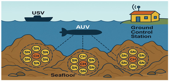
Figure 1. Overview of the UASN system with sensor nodes (SNs) on an uneven seafloor.

To facilitate communication, a clustering method is applied to group the sensor nodes into $M$ clusters. One node in each cluster is designated as a cluster head (CH), forming a set of $M$ CHs labelled as $i=1,2,\dots ,M$ [5]. The set of CHs can be reselected in each data collection round to balance energy consumption among nodes, using methods such as those presented in [6,7,13,38,39]. Each CH collects data from the sensor nodes within its cluster and transmits it to the AUV. Given the focus on AUV trajectory planning, this paper considers only CH–AUV communication and assumes that data transmission from sensor nodes to CHs has already been completed.

The AUV navigates along a horizontal plane above the CHs to collect their aggregated data. Upon mission completion, the AUV offloads the collected data to a USV, which serves as the surface sink [1]. The USV then relays the data to a ground control station using radio communication. This study specifically focuses on the data transmission process from the underwater CHs to the USV [1].

2.1.2. AUV Kinematic Model

Consider an AUV fitted with suitable receivers and deployed to perform data collection tasks in a UASN. The AUV begins its mission at the surface point $S_s=(x_{{USV}_s},y_{{USV}_s},0)$, where the USV is initially stationed. It then descends to a predefined depth $z_d$, navigates along a horizontal plane to collect data from the CHs, and finally returns to the USV at a different surface location $S_f=(x_{{USV}_f},y_{{USV}_f},0)$. The depth $z_d$ of the horizontal plane must satisfy the constraint:

$$z_d\le 0,$$

(1)

to ensure the AUV remains below the sea surface. Additionally, $z_d$ must be selected such that its vertical distance from the highest point of the seafloor, denoted by $\delta \left(t\right)$, is greater than a safety distance ${\delta }_{safe}$ and within the allowable depth range of the AUV at:

$$\delta \left(t\right)>{\delta }_{safe} \forall t\in [0,T],$$

(2)

where $T$ denotes the total duration of the mission. This constraint in (2) ensures that the AUV does not descend close to the seafloor, even in the most challenging terrain conditions. The kinematic equations describing the AUV’s motion in the horizontal plane are given by [17]:

$$\dot{x}\left(t\right)=u\left(t\right) \mathrm{c}\mathrm{o}\mathrm{s} \psi \left(t\right)$$

$$\dot{y}\left(t\right)=u\left(t\right)\sin \psi \left(t\right)$$

$$\dot{z}\left(t\right)=\omega \left(t\right)$$

$$\dot{\psi }\left(t\right)=r\left(t\right).$$

(3)

The AUV’s state at time $t$ is defined by its position $\left(x\right(t), y(t), z(t\left)\right)$, where $z\left(t\right)=z_d$ and its yaw angle $\psi \left(t\right)\in [0, 2\pi )$. Its motion is governed by three key control inputs: the surge speed $u\left(t\right)\in (0,u_{\max }]$, the heave speed $\omega \left(t\right)\in (0,{\omega }_{\max }]$, and yaw rate $r\left(t\right)\in [-r_{\max }, r_{\max }]$. When the yaw rate $\omega \left(t\right)$ is nonzero, the AUV follows a curved path with a turning radius defined as:

$${\kappa }_i\left(t\right)=\left({\displaystyle \frac{u\left(t\right)}{\left|r\left(t\right)\right|}}\right).$$

(4)

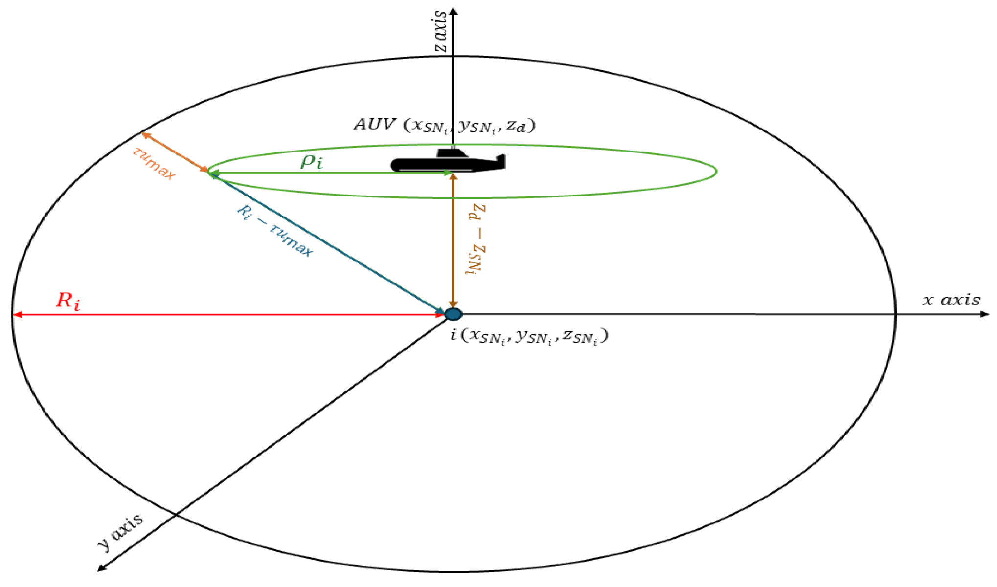
2.1.3. Communication Region Model

Let the coordinates of the CHs be denoted as $(x_{{CH}_i}, y_{{CH}_i}, z_{{CH}_i})$, for $i=1,2,\dots ,M$. These CHs are stationary; however, their depth values $z_{{CH}_i}$ vary due to deployment over an uneven seafloor. Each CH communicates using acoustic signals and can connect with the AUV within a communication range $R_i>0$ [11]. Within this communication region, data transmission between the AUV and the corresponding CH takes place.

Although transmission time may vary due to factors such as distance, data size, and channel quality, this study simplifies the model by assuming a fixed transmission duration for all CHs [6,7]. Let $\tau >0$ denote the minimum time the AUV must remain within the communication range of any CH $i$ to successfully complete data transmission. A successful connection with CH $i$ is said to be established at time $t_i$ if, during the interval $[t_i-\tau , t_i]$, the AUV remains within the communication region $R_i$. This means that the distance $d_i\left(t\right)$ between the AUV and CH $i$ must satisfy $d_i\left(t\right)\le R_i$ for all $t$ in that period.

Given that the maximum surge speed of the AUV is $u_{\max }$, it cannot move more than $\tau u_{\max }$ meters in $\tau$ seconds. Therefore, if the AUV is within a distance of $R_i-\tau u_{\max }$ from CH $i$ at time $t_i$, it is guaranteed to remain within the full communication sphere of radius $R_i$ during the interval $[t_i-\tau ,t_i]$. The corresponding horizontal constraint on the AUV’s position, projected onto the plane $z\left(t\right)=z_d$, is given by:

$${\rho }_i=\sqrt{{\left(R_i-\tau u_{\max }\right)}^2-{\left(z_d-z_{{CH}_i}\right)}^2}.$$

(5)

If the AUV lies within a circle of radius ${\rho }_i$, centered at $(x_{{CH}_i},y_{{CH}_i},z_d)$ at time $t_i$, its 3D distance to node $i$ is less than $R_i-\tau u_{\max }$. This ensures that the AUV remains within the communication range for the entire duration $\tau$, enabling a successful data transmission (refer to Figure 2). This condition holds under the assumption:

$$R_i>\left|z_d-z_{{CH}_i}\right|+\tau u_{\max } \forall i,$$

(6)

which guarantees that the square root is real, and the projected region is nonempty.

Figure 2. The design of the horizontal communication region for sensor node i.

It is important to note that Equation (5) shows that as the vertical distance between the CH’s altitude $z_{{CH}_i}$ and the AUV’s altitude $z_d$ decreases, the radius ${\rho }_i$ of the horizontal communication circle increases. This increase in ${\rho }_i$ allows the AUV to maintain a greater horizontal distance from the CH while still successfully completing the data transmission. In the context of an uneven seafloor, this is beneficial because a larger ${\rho }_i$ reduces the need for the AUV to approach the uneven terrain of the seafloor where the CH is located, hence lowering the risk of collision. Thus, in addition to satisfying constraint (2), Equation (5) implicitly contributes to collision avoidance by enabling communication at a safer distance from CHs located on elevated regions of the seafloor.

2.2. Problem Formulation

This subsection presents the mathematical formulation of the trajectory planning problem, establishing the foundation for the proposed solution.

2.2.1. Objective Function

This work investigates the problem of planning an optimal trajectory for a single AUV assigned to collect data from $M$ CHs deployed across the UASN. The AUV begins and ends its mission at two distinct surface locations, $S_s$ and $S_f$, both associated with a USV. The objective is to determine the optimal starting and ending locations, along with the most efficient visiting sequence of CHs and corresponding waypoints, such that the total residual VoI of the collected data is maximized. This enables the timely delivery of critical information to the USV for rapid response to abnormal events.

Several studies [6,7,8,9,11] have proposed different VoI definitions for underwater data, considering importance, timeliness, and rarity. In this paper, we adopt a model similar to that in [1], which classifies data as emergency or routine and utilizes an adaptive decay function that links value loss to data significance. It also computes the initial VoI based on historical data, offering a practical and realistic approach [1].

To illustrate the adopted VoI concept, consider a typical underwater pipeline surveillance scenario. Emergency events such as leaks are often indicated by sudden pressure drops or abnormal chemical readings [6,9]. In contrast to routine measurements, these events are rare and carry high importance, requiring urgent data transmission to prevent serious consequences. In such cases, a normal distribution can be applied to historical data to capture the rarity and significance of these events when calculating the VoI [1].

Let $C$ denote the set of measured data, where $C_{kj}$ represents the $k$-th reading obtained by the $j$-th sensor node in cluster $i$. Here $k=1,2,\dots$, and $j=1,2,\dots ,U$. Each sensor node $j$ maintains historical data characterized by a mean ${\mu }_j$ and standard deviation ${\sigma }_j$. The abnormality of a reading is quantified using an importance score $\mathcal{I}\left(C_{kj}\right)$, defined as [1]:

$$\mathcal{I}\left(C_{kj}\right)={\displaystyle \frac{1}{{\sigma }_j\sqrt{2\pi }}}{\int }_{-\infty }^{{\mu }_j+\left|C_{kj}-{\mu }_j\right|}{e}^{{\displaystyle \frac{-{(c-{\mu }_j)}^2}{2{{\sigma }_j}^2}}}dc,$$

(7)

where $c$ is the integral variable. Equation (7) captures the degree of deviation of a reading $C_{kj}$ from the historical norm. The most abnormal reading from sensor node $j$ is determined as $\mathcal{I}\left(C_j\right)={\max }_k\left\{\mathcal{I}\left(C_{kj}\right)\right\}$ [1]. The CH then computes the cluster’s data importance as ${\mathcal{I}}_i={\max }_j\left\{\mathcal{I}\left(C_j\right)\right\}$ based on the data received from all sensor nodes, to identify the most important data in cluster $i$ [1].

At this point, the initial VoI corresponding to the data from cluster $i$, denoted by ${\mathcal{V}}_{{int}_i}$, is calculated using [1]:

$${\mathcal{V}}_{{int}_i}=2 {\mathcal{I}}_i-1.$$

(8)

Equation (8) highlights the relationship between data abnormality and its importance, where a higher value of ${\mathcal{V}}_{{int}_i}$ indicates higher urgency of the data [1]. To reflect how urgency decreases over time, a decay-based VoI model is constructed. When the AUV collects data with initial VoI ${\mathcal{V}}_{{int}_i}$ from CH $i$ and delivers it to the USV at time $t_c$, the residual VoI is computed as [1]:

$$V_{r_i}\left(t_c\right)={{\mathcal{V}}_{{int}_i}(1-\beta {\mathcal{I}}_i)}^{t_c},$$

(9)

where $\beta$ is the decay coefficient and $t_c$ is the time duration from the start of data collection to its delivery to the USV. Equation (9) reflects that data with higher abnormality, i.e., greater deviation from historical norms $\left|C_{kj}-{\mu }_j\right|,$ undergoes more rapid value decay [1]. Hence, the objective is to plan a trajectory that preserves the maximum possible residual VoI.

To enable trajectory planning for residual VoI maximization, let ${\mathcal{C}}_i$ denote a horizontal circle of radius ${\rho }_i$ around each CH, centered at $(x_{{CH}_i},y_{{CH}_i},z_d)$, for each $i=1,2,\dots ,M$. This circle defines the horizontal communication region within which the AUV can successfully transmit data to CH $i$ at the horizontal plane $z=z_d$. Furthermore, define ${\mathcal{B}}_i$ as the corresponding closed disk with the same center and radius. It is assumed that for any given index $i$, there exists at least one index $\alpha \ne i$, with $\alpha \in \{1,2,\dots ,M\}$, such that:

$${\mathcal{B}}_i\bigcap {\mathcal{B}}_{\alpha }=\varphi .$$

(10)

Let ${\mathcal{Q}}_i=\{q_{1_i},q_{2_i},\dots ,q_{L_i}\}$, where $q_{l_i}=(x_{q_{l_i}},y_{q_{l_i}},z_d)$ for $l=1,2,\dots ,L$, be a finite set of $L$ candidate waypoints uniformly distributed along the circumference of the horizontal circle ${\mathcal{C}}_i$. Each $q_{l_i}\in {\mathcal{C}}_i$ lies at a horizontal distance ${\rho }_i$ from the center. The AUV must visit one waypoint per CH, and the sequence in which the CHs are visited significantly affects the overall performance due to information decay over time.

Let $\widehat{\mathsf{\Phi }}$ denote the set of all permutations of the index set $\{1,2,\dots ,M\}$, which contains $M$! elements. Each permutation $\mathsf{\Phi }=(s\left(1\right),s\left(2\right),\dots ,s\left(M\right))$, where $\mathsf{\Phi }\in \widehat{\mathsf{\Phi }}$, represents a unique visiting sequence of the $M$ circles. For each permutation $\mathsf{\Phi }$, the set of all possible combinations of candidate waypoints, one per CH, is defined as the Cartesian product:

$${\mathcal{Q}}_{\Phi }={\mathcal{Q}}_{s\left(1\right)}\times {\mathcal{Q}}_{s\left(2\right)}\times \cdot \cdot \cdot \times {\mathcal{Q}}_{s\left(M\right)}.$$

(11)

This results in $L^M$ candidate paths. Each element $\mathcal{P}\in {\mathcal{Q}}_{\mathsf{\Phi }}$ is a candidate trajectory comprising one waypoint per CH, ordered according to the sequence $\mathsf{\Phi }$:

$$\mathcal{P}=(q_{l_{s\left(1\right)}},q_{l_{s\left(2\right)}},\dots ,q_{l_{s\left(M\right)}}),$$

(12)

where $q_{l_{s\left(i\right)}}\in {\mathcal{Q}}_{s\left(i\right)}$ is the selected waypoint for CH $s\left(i\right)$ in the sequence.

Building on the above definitions, the primary objective function is formulated as follows:

$$\underset{\Phi ,\mathcal{P}}{\max }{\sum }_{i=1}^M{V}_{r_i}\left(t_c\right)={\sum }_{i=1}^M{{\mathcal{V}}_{{\mathrm{int}}_i}(1-\beta {\mathcal{I}}_i)}^{t_c}.$$

(13)

The AUV trajectory planning problem is thus defined as the task of selecting the optimal visiting sequence of CHs, along with their corresponding data collection waypoints, in order to maximize the objective function in (13). It is assumed that the AUV has complete knowledge of the VoI associated with each CH at the start of the mission from its initial surface position $S_s$.

2.2.2. Problem Statement

This paper addresses the problem of selecting surface points $S_s$ and $S_f$, and planning a trajectory for the AUV (3) that starts at $S_s$, traverses a sequence of waypoints to collect data from the $M$ CHs, and ends at $S_f$, such that the objective function (13) is maximized, subject to constraints (1), (2), and (6).

2.3. Proposed Solution

This subsection outlines the proposed solution, including the AUV trajectory optimization algorithm and the path design for feasible movement between waypoints.

2.3.1. AUV Trajectory Optimization Algorithm

To solve the trajectory planning problem defined in (13), this work proposes a forward DP approach that maximizes the total residual VoI collected during the mission. The method simultaneously determines the optimal sequence for visiting the $M$ CHs and selects one waypoint per CH from a candidate set located along its horizontal communication circle of radius ${\rho }_i$. It systematically explores all feasible combinations of CH visiting orders and waypoint assignments while accounting for travel time, data degradation, and AUV motion constraints. A complete summary of the algorithm is provided in Algorithm 1.

Given each combination $(\mathsf{\Phi },\mathcal{P})$, the travel time between consecutive waypoints is computed using the kinematic model in (3) and the path design strategy described in the next section. In this work, the residual VoI is evaluated over the time interval beginning with the AUV’s arrival at the first CH and ending upon its return to the USV at the end of the mission. Accordingly, the forward DP algorithm searches for the optimal waypoint sequence and selection that maximizes the total residual VoI over this operational window.

Algorithm 1. Forward DP-based Algorithm for AUV Trajectory Optimization
Input: Candidate waypoint sets {${\mathcal{Q}}_1, {\mathcal{Q}}_2,\dots , {\mathcal{Q}}_M$}, all permutations $\mathsf{\Phi }\in \widehat{\mathsf{\Phi }}$, VoI parameters: ${\mathcal{V}}_{{\mathrm{int}}_i}$ and ${\mathcal{I}}_i$ for each CH i, decay factor β.
Output: Optimal CH visit sequence ${\mathsf{\Phi }}_{\mathrm{opt}}$, optimal waypoint path ${\mathcal{P}}_{\mathrm{opt}}$, and maximum total residual VoI $V_{{r\mathrm{totalBest}}_{\mathsf{\Phi }}}$.
1	Initialize $V_{{r\mathrm{totalBest}}_{\mathsf{\Phi }}}:=-\mathrm{\infty }$
2	for each permutation $\mathsf{\Phi }=(s\left(1\right),s\left(2\right),\dots ,s\left(M\right))\in \widehat{\mathsf{\Phi }}$:
3	for stage i = 1
4	for each $q\in {\mathcal{Q}}_{s\left(1\right)}$:
5	Compute $t_q=t_{s\to q}$
6	Compute residual VoI: $V_{r_{s\left(1\right)}}\left(t_q\right)={{\mathcal{V}}_{{\mathrm{int}}_{s\left(1\right)}}(1-\beta {\mathcal{I}}_{s\left(1\right)})}^{t_q}$
7	Set $J\left(1,q\right):=V_{r_{s\left(1\right)}}\left(t_q\right)$  $\mathrm{and} \mathrm{Prev}(1,q):=S_s$
8	for i = 2 to M:
9	for each $q\in {\mathcal{Q}}_{s\left(i\right)}$:
10	for each $\acute{q}\in {\mathcal{Q}}_{s(i-1)}$:
11	Compute travel time: $t_{\acute{q\to }q}$
12	Compute arrival time: $t_q=t_{\acute{q}}+t_{\acute{q\to }q}$
13	Compute new VoI: $V_{r_{s\left(i\right)}}\left(t_q\right)={{\mathcal{V}}_{{\mathrm{int}}_{s\left(i\right)}}(1-\beta {\mathcal{I}}_{s\left(i\right)})}^{t_q}$
14	Update $J(i,q):=\underset{\acute{q}\in {\mathcal{Q}}_{s\left(i-1\right)}}{\max }[J\left(i-1,\acute{q}\right)+V_{r_{s\left(i\right)}}(t_q)]$
15	Store $\mathrm{Prev}(i,q):=\acute{q}$
16	Compute upper bound ${\Gamma }_{\mathrm{up}}(i,q)=\sum _{a=i+1}^M{\mathcal{V}}_{{\mathrm{int}}_{s\left(a\right)}}$
17	If ${J\left(i,q\right)+\Gamma }_{\mathrm{up}}(i,q)<V_{{r\mathrm{totalBest}}_{\mathsf{\Phi }}}$: prune path
18	After stage M, find $q\in {\mathcal{Q}}_{s\left(M\right)}\mathrm{maximizing} J(M,q)$
19	If a new maximum is found, update  $V_{{r\mathrm{totalBest}}_{\mathsf{\Phi }}}$ and record ${\mathsf{\Phi }}_{\mathrm{opt}}$
20	Backtrack from final q using $\mathrm{Prev}(i,q)$ to build ${\mathcal{P}}_{\mathrm{opt}}$
21	Return ${\mathsf{\Phi }}_{\mathrm{opt}}, {\mathcal{P}}_{\mathrm{opt}}$ and $V_{{r\mathrm{totalBest}}_{\mathsf{\Phi }}}$

The core of the proposed solution is the forward DP approach that incrementally constructs the optimal trajectory. The use of a forward DP formulation is essential in this context, as the residual VoI associated with each CH progressively decays over time. Since the reward collected at each waypoint directly depends on its visitation time, the algorithm must traverse the decision space in the same direction as time progresses. This forward traversal enables accurate tracking of elapsed time and proper application of the corresponding VoI decay at each stage. A similar forward DP approach has also been employed in [24].

In this paper, the aim is to evaluate the residual VoI collected from the first CH to the USV’s final position. However, the forward DP procedure is initiated from the AUV’s surface start location $S_s$ and progresses through the visitation sequence, terminating at the final CH. This modeling choice is justified by the symmetry in vertical travel time between the descent from $S_s$ and the ascent to $S_f$. Specifically, these segments are represented as vertical motions at a constant heave speed between the surface $z=0$ and the operational depth $z=z_d$, starting from and ending at waypoints that share the same horizontal coordinates as $S_s$ and $S_f$, respectively. As this vertical traversal time remains constant across all trajectory candidates, it results in a uniform decay period for this portion of the mission. This symmetry ensures a consistent basis for evaluating and comparing all candidate trajectories.

Given the permutation $\mathsf{\Phi }=(s\left(1\right),s\left(2\right),\dots ,s\left(M\right))$, which defines the order of visiting the $M$ CHs, the algorithm constructs a DP table $J(i, q_{l_{s\left(i\right)}})$. Here, $i \in \{1,2,\dots , M\}$ denotes the current stage, and $q_{l_{s\left(i\right)}}$ is a candidate waypoint on ${\mathcal{C}}_{s\left(i\right)}$ around CH $s\left(i\right)$. The value $J(i, q_{l_{s\left(i\right)}})$ stores the maximum cumulative residual VoI collected up to CH $s\left(i\right)$ when the AUV arrives at waypoint $q_{l_{s\left(i\right)}}$. To keep the notation simpler, we use $J(i, q)$ to represent $J(i, q_{l_{s\left(i\right)}})$, where $q\in {\mathcal{Q}}_{s\left(i\right)}$.

At stage $i=1$, the residual VoI for each candidate waypoint $q\in {\mathcal{Q}}_{s\left(1\right)}$ is determined based on the travel time from the initial point $S_s$. Note that if $q=(x_{q_{l_{s\left(1\right)}}},y_{q_{l_{\left(1\right)}}},z_d)$, then the corresponding surface starting point is $S_s=(x_{q_{l_{s\left(1\right)}}},y_{q_{l_{\left(1\right)}}},0)$. The arrival time at $q$, denoted by $t_q$, is computed as the time taken to travel from $S_s$ to $q$, i.e., ${t_q=t}_{s\to q}$. This arrival time is then used to evaluate the residual VoI at $q$. The corresponding residual VoI is:

$$V_{r_{s\left(1\right)}}\left(t_q\right)={{\mathcal{V}}_{{int}_{s\left(1\right)}}(1-\beta {\mathcal{I}}_{s\left(1\right)})}^{t_q}.$$

(14)

This initializes the DP table as:

$$J\left(1, q\right):=V_{r_{s\left(1\right)}}\left(t_q\right),$$

(15)

and the backtracking information is initialized as $\mathrm{Prev}(1,q) :=S_s$.

For each subsequent stage $i=2,\dots M$, and for every candidate waypoint $q\in {\mathcal{Q}}_{s\left(i\right)}$, the algorithm iteratively evaluates all possible transitions from all previous waypoints $\acute{q}\in {\mathcal{Q}}_{s(i-1)}$. The travel time between the two waypoints is denoted by $t_{\acute{q\to }q}$, indicating the time required to move from $\acute{q}$ to $q$. The updated arrival time at $q$ is then calculated as:

$$t_q=t_{\acute{q}}+t_{\acute{q\to }q},$$

(16)

where $t_{\acute{q}}$ is the stored arrival time at the previous waypoint $\acute{q}$. The residual VoI collected at CH $s\left(i\right)$ upon arriving at $q$ is evaluated as:

$$V_{r_{s\left(i\right)}}\left(t_q\right)={{\mathcal{V}}_{{int}_{s\left(i\right)}}(1-\beta {\mathcal{I}}_{s\left(i\right)})}^{t_q}.$$

(17)

The DP table is subsequently updated by selecting the transition from $\acute{q}$ that results in the maximum total residual VoI:

$$J(i, q) :=\underset{\acute{q}\in {\mathcal{Q}}_{s\left(i-1\right)}}{\max }[ J\left(i-1, \acute{q}\right)+V_{r_{s\left(i\right)}}(t_q)].$$

(18)

During each step, the algorithm updates $\mathrm{Prev}(i,q)$ with the previous waypoint $\acute{q}$ that results in the maximum value, i.e., $\mathrm{Prev}(i,q) :=\acute{q}$. This enables recovery of the optimal waypoint sequence via backtracking once the process is complete.

At the final stage, the optimal value corresponding to the current permutation Φ is determined as:

$$V_{{\mathrm{r}\mathrm{total}}_{\Phi }}=\underset{q\in {\mathcal{Q}}_{s\left(M\right)}}{\max }J(M,q).$$

(19)

Following this step, the optimal waypoint sequence is recovered by backtracking through the stored transitions starting from the final waypoint. This procedure is repeated for each permutation $\mathsf{\Phi }\in \widehat{\mathsf{\Phi }}$, and the optimal path is determined as:

$$({\Phi }_{\mathrm{opt}},{\mathcal{P}}_{\mathrm{opt}})=\underset{\Phi \in \widehat{\Phi }}{\mathrm{argmax}}{V}_{{\mathrm{r}\mathrm{total}}_{\Phi }}.$$

(20)

Here, ${\mathsf{\Phi }}_{\mathrm{opt}}$ denotes the optimal CH visiting sequence, and ${\mathcal{P}}_{\mathrm{opt}}$ represents the corresponding set of selected waypoints. The AUV’s surface start and end positions, $S_s$ and $S_f$, which align with the USV’s start and end positions, are determined from the first and last waypoints in ${\mathcal{P}}_{\mathrm{opt}}$, respectively. These surface positions are obtained by setting the $z$-coordinates of the respective waypoints to zero, ensuring they lie on the water surface. Consequently, the USV is positioned directly above the AUV’s initial waypoint at mission start and above the final waypoint at mission end, thereby completing the construction of the optimal trajectory.

It is important to note that, while the ascent segment does not influence the optimization outcome, a post-processing correction may be applied if the residual VoI is to be evaluated over the entire mission duration, from the USV’s start to end positions. The decay incurred during this final vertical segment can then be incorporated by adjusting the residual VoI based on the arrival time at the last waypoint and the known ascent duration.

To address the high complexity of exploring all CH visit permutations and waypoint combinations, this paper applies a pruning approach based on an estimated upper bound of the remaining residual VoI. The idea follows the principles presented in [40,41] and enables the forward DP algorithm to discard unpromising solutions early in the recursion. As a result, the computational burden is significantly reduced without compromising optimality.

At stage $i$, $J(i, q)$ is defined as the total residual VoI accumulated after the AUV has visited CHs $s\left(1\right),s\left(2\right),\dots ,s\left(i\right)$ and is currently located at waypoint $q\in {\mathcal{Q}}_{s\left(i\right)}$. For each such DP state, we introduce an upper bound function ${\mathsf{\Gamma }}_{\mathrm{up}}(i, q)$, which estimates the maximum residual VoI achievable from the remaining CHs $s(i+1),s(i+2),\dots ,s\left(M\right)$, under ideal travel conditions and assuming no information decay. The adopted upper bound is given by:

$${\Gamma }_{\mathrm{up}}(i, q)={\sum }_{a=i+1}^M{\mathcal{V}}_{{int}_{s\left(a\right)}}.$$

(21)

Assuming instant access with no decay, this optimistic estimate in (21) safely bounds the remaining value and avoids early pruning. Let $V_{{r\mathrm{totalBest}}_{\mathsf{\Phi }}}$ denote the global lower bound, defined as the maximum total residual VoI from any fully evaluated trajectory. At each DP stage, the pruning condition is applied as:

$${J\left(i,q\right)+\Gamma }_{\mathrm{up}}(i, q)<V_{{\mathrm{r}\mathrm{totalBest}}_{\mathsf{\Phi }}}.$$

(22)

If the condition in (22) holds, then, even under ideal assumptions, the current trajectory cannot outperform the best solution identified so far. In such cases, the algorithm safely prunes the current permutation and skips the remaining stages of its evaluation. This strategy significantly reduces the number of trajectory branches that must be explored, particularly during the later stages of recursion, where the computational cost of full evaluation is highest. As a result, the algorithm achieves a substantial improvement in runtime efficiency while preserving optimality within the reduced search space.

2.3.2. Path Design

After determining the optimal sequence of waypoints that maximizes the residual VoI from all $M$ CHs, the next step is to develop a trajectory design method based on the AUV’s kinematic model. In this section, we design the path of the AUV to navigate through the selected waypoints, starting from the initial USV position $S_s$ and ending at the final USV position $S_f$ and determine the control input values required for its motion. Knowing these values enables the calculation of the travel time between waypoints, which is essential for implementing the forward DP algorithm.

Let the optimal waypoint set be denoted as ${\mathcal{P}}_{\mathrm{opt}}=\{q_{l_{s^{\mathrm{opt}}\left(1\right)}}^{\mathrm{opt}},\dots , q_{l_{s^{\mathrm{opt}}\left(M\right)}}^{\mathrm{opt}}\}\in {\mathcal{Q}}_{{\mathsf{\Phi }}_{\mathrm{opt}}}$, where $q_{l_{s^{\mathrm{opt}}\left(i\right)}}^{\mathrm{opt}}\in {\mathcal{Q}}_{s^{\mathrm{opt}}\left(i\right)}$ represents the selected waypoint from the $i$-th CH in the optimal permutation ${\mathsf{\Phi }}_{\mathrm{opt}}=\{s^{\mathrm{opt}}\left(1\right),\dots ,s^{\mathrm{opt}}\left(M\right)\}$, and each waypoint is defined as $q_{l_{s^{\mathrm{opt}}\left(i\right)}}^{\mathrm{opt}}=(x_{q_{l_{s^{\mathrm{opt}}\left(i\right)}}}^{\mathrm{opt}},y_{q_{l_{s^{\mathrm{opt}}\left(i\right)}}}^{\mathrm{opt}},z_d)$. Accordingly, the AUV starts from the surface location $S_s=(x_{q_{l_{s^{\mathrm{opt}}\left(1\right)}}}^{\mathrm{opt}},y_{q_{l_{s^{\mathrm{opt}}\left(1\right)}}}^{\mathrm{opt}},z_d)$, descends vertically to the first waypoint $q_{l_{s^{\mathrm{opt}}\left(1\right)}}^{\mathrm{opt}}$, and then follows a horizontal trajectory through all waypoints in ${\mathcal{P}}_{\mathrm{opt}}$. Once the final waypoint $q_{l_{s^{\mathrm{opt}}\left(M\right)}}^{\mathrm{opt}}$ is reached, the AUV ascends vertically to the surface location $S_f=(x_{q_{l_{s^{\mathrm{opt}}\left(M\right)}}}^{\mathrm{opt}},y_{q_{l_{s^{\mathrm{opt}}\left(M\right)}}}^{\mathrm{opt}},z_d)$.

For simplicity, we define a new set $P_{final}=\{p_1,\dots ,p_F\}$, representing the complete sequence of points along the AUV’s path, where the indices are labeled by $\gamma =1,\dots ,F$ and $F=M+2$. This set includes the starting point $S_s$, all waypoints in ${\mathcal{P}}_{\mathrm{opt}}$, and the final point $S_f$. Since we are navigating between discrete waypoints, control inputs are determined for each subtrajectory connecting two consecutive points. Specifically, to move from point $p_{\gamma }$ to point $p_{\gamma +1}$, the control inputs $u_{\gamma }$, ${\omega }_{\gamma }$, and $r_{\gamma }$ are determined, enabling calculation of the corresponding travel time and transition dynamics required for the forward DP algorithm.

The AUV follows a trajectory composed of three phases: a vertical descent from $p_1=S_s$ to $p_2$; horizontal movement through the waypoints $p_2,\dots ,p_{F-1}$ along the horizontal plane at depth $z_d$, and a vertical ascent from $p_{F-1}$ to $p_F=S_f$. During the vertical phases, the control inputs $u_{\gamma }$ and $r_{\gamma }$ are set to zero, while ${\omega }_{\gamma }$ is set to −${\omega }_{\max }$ for descent and ${\omega }_{\max }$ for ascent.

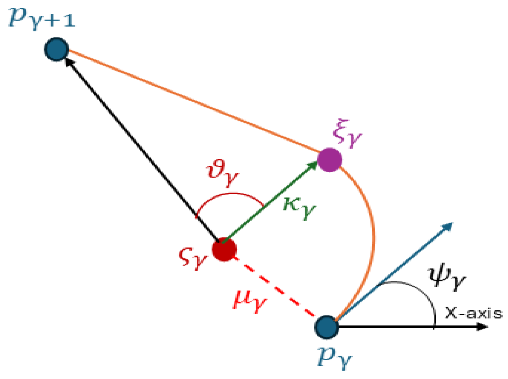
For the horizontal movement, the AUV follows a Dubins-like trajectory design adapted from [24], combining a single arc turn with a straight segment to meet its kinematic constraints. The AUV rotates from its current waypoint $p_{\gamma }$ at a constant yaw rate $r_{\gamma }$, selecting either $r_{\max }$ or $-r_{\max }$ for $\gamma =2,\dots ,F-1$. Rotation continues until the heading ${\psi }_{\gamma }$ aligns with the vector leading to the subsequent waypoint $p_{\gamma +1}$, reaching the tangent point ${\xi }_{\gamma }$ (see Figure 3). At ${\xi }_{\gamma }$, the yaw rate $r_{\gamma }$ is set to zero, and the AUV proceeds straight toward $p_{\gamma +1}$ [24]. Rotation is necessary only if the current heading ${\psi }_{\gamma }$ is misaligned with the direction to $p_{\gamma +1}$; otherwise, $r_{\gamma }$ is set to zero without rotation.

Figure 3. The AUV trajectory design.

Throughout this phase, $r_{\gamma }$ is the only variable control input, which only employed when rotation is necessary. The surge speed is maintained constant at $u_{\gamma }=u_{\max }$ throughout the entire horizontal movement, while the heave speed ${\omega }_{\gamma }$ is set to zero, as there is no vertical movement.

The selection between $r_{\max }$ or $-r_{\max }$ is determined by computing the angle ${\eta }_{\gamma }\in [0,2\pi )$, measured counterclockwise from the x-axis to the vector $\overrightarrow{p_{\gamma }{p}_{\gamma +1}}$. The direction of rotation is then decided by evaluating the angular difference ${\eta }_{\gamma }-{\psi }_{\gamma }\in (-2\pi ,2\pi )$, representing the counterclockwise angle between the AUV’s current heading and the vector $\overrightarrow{p_{\gamma }{p}_{\gamma +1}}$. Based on the evaluated angular difference, the appropriate rotation direction is selected as follows [24]:

$$\left\{\begin{array}{c}no turn, if {\eta }_{\gamma }-{\psi }_{\gamma }=0 \\ turn right, if {\eta }_{\gamma }-{\psi }_{\gamma }\in \left[-\pi ,0\right)\cup [\pi ,2\pi )\\ turn left, if {\eta }_{\gamma }-{\psi }_{\gamma }\in (-2\pi ,-\pi )\cup (0,\pi )\end{array}\right..$$

(23)

To find the position of the tangent point ${\xi }_{\gamma }$ where the AUV stops rotating, a unit vector ${\mu }_{\gamma }$ perpendicular to the current heading ${\psi }_{\gamma }$ is first defined. This vector is used to determine the center ${\varsigma }_{\gamma }$ of the AUV’s circular path, such that ${\varsigma }_{\gamma }$ lies at a distance ${\kappa }_{\gamma }$ from the current position $p_{\gamma }$ along the direction of ${\mu }_{\gamma }$ [24]. Two vectors, $\overrightarrow{{\varsigma }_{\gamma }{p}_{\gamma }}$ and $\overrightarrow{{\varsigma }_{\gamma }{\xi }_{\gamma }}$, represent the directions from ${\varsigma }_{\gamma }$ to $p_{\gamma }$ and ${\xi }_{\gamma }$, respectively. The center ${\varsigma }_{\gamma }$ is computed as [24]:

$${\varsigma }_{\gamma }=p_{\gamma }+{\displaystyle \frac{u_{\gamma }}{r_{\max }}}{\mu }_{\gamma }.$$

(24)

Since the tangent vector $\overrightarrow{{\xi }_{\gamma }{p}_{\gamma +1}}$ is orthogonal to $\overrightarrow{{\varsigma }_{\gamma }{\xi }_{\gamma }}$, their dot product is zero [24].

Moreover, given that $\overrightarrow{{\varsigma }_{\gamma }{\xi }_{\gamma }}$ has magnitude ${\kappa }_{\gamma }$, where ${\kappa }_{\gamma }={\displaystyle \frac{u_{\gamma }}{r_{\max }}}$, and that the tangent vector can be expressed as $\overrightarrow{{\xi }_{\gamma }{p}_{\gamma +1}}=\overrightarrow{{\varsigma }_{\gamma }{p}_{\gamma +1}}-\overrightarrow{{\varsigma }_{\gamma }{\xi }_{\gamma }}$, the orthogonality condition leads to [24]:

$$\overrightarrow{{\varsigma }_{\gamma }{\xi }_{\gamma }}\cdot \left(\overrightarrow{{\varsigma }_{\gamma }{p}_{\gamma +1}}-\overrightarrow{{\varsigma }_{\gamma }{\xi }_{\gamma }}\right)=0.$$

(25)

Now, using (25) the angle between $\overrightarrow{{\varsigma }_{\gamma }{\xi }_{\gamma }}$ and $\overrightarrow{{\varsigma }_{\gamma }{p}_{\gamma +1}}$ is computed as:

$${\vartheta }_{\gamma }=\arccos \left({\displaystyle \frac{\frac{u_{\gamma }}{r_{\max }}}{\left|p_{\gamma +1}-{\varsigma }_{\gamma }\right|}}\right).$$

(26)

Using ${\vartheta }_{\gamma }$ from (26), the unit vector $\overrightarrow{{\varsigma }_{\gamma }{\xi }_{\gamma }}$ can be derived by rotating the unit vector $\overrightarrow{{\varsigma }_{\gamma }{p}_{\gamma +1}}$ counterclockwise by ${\vartheta }_{\gamma }$, as follows [24]:

$${\displaystyle \frac{\overrightarrow{{\varsigma }_{\gamma }{\xi }_{\gamma }}}{\left|\overrightarrow{{\varsigma }_{\gamma }{\xi }_{\gamma }}\right|}}=\left[\begin{array}{cc}\cos {\vartheta }_{\gamma }& -\sin {\vartheta }_{\gamma }\\ \sin {\vartheta }_{\gamma }& \cos {\vartheta }_{\gamma }\end{array}\right] {\displaystyle \frac{\overrightarrow{{\varsigma }_{\gamma }{p}_{\gamma +1}}}{\left|\overrightarrow{{\varsigma }_{\gamma }{p}_{\gamma +1}}\right|}}.$$

(27)

From $\overrightarrow{{\varsigma }_{\gamma }{\xi }_{\gamma }}={\xi }_{\gamma }-{\varsigma }_{\gamma }$, ${\kappa }_{\gamma }=\overrightarrow{{\varsigma }_{\gamma }{\xi }_{\gamma }}={\displaystyle \frac{u_{\gamma }}{r_{\max }}}$, along with (24), the tangent point ${\xi }_{\gamma }$ is expressed as [24]:

$${\xi }_{\gamma }={\varsigma }_{\gamma }+{\displaystyle \frac{u_{\gamma }}{r_{\max }}}\left[\begin{array}{cc}\cos {\vartheta }_{\gamma }& -\sin {\vartheta }_{\gamma }\\ \sin {\vartheta }_{\gamma }& \cos {\vartheta }_{\gamma }\end{array}\right]\times {\displaystyle \frac{p_{\gamma +1}-{\varsigma }_{\gamma }}{\left|p_{\gamma +1}-{\varsigma }_{\gamma }\right|}}.$$

(28)

The tangent point ${\xi }_{\gamma }$, as given in (28), is considered feasible if the vector from ${\xi }_{\gamma }$ to $p_{\gamma +1}$ aligns with the AUV’s departure direction at ${\xi }_{\gamma }$. If this condition is not satisfied, ${\vartheta }_{\gamma }$ is replaced by ${-\vartheta }_{\gamma }$, and a new ${\xi }_{\gamma }$ is selected [24].

3. Results and Discussion

This section evaluates the performance of the proposed method through MATLAB simulations. The results demonstrate its effectiveness in selecting optimal USV start and end positions and in generating an AUV trajectory that enables efficient data collection in UASNs for IoUT applications, while maximizing the total residual VoI. The AUV preserves approximately 64–70% of the total residual VoI upon returning to the USV.

Benchmarking is essential to demonstrate the performance of the proposed method. However, direct comparison with some related approaches is limited due to substantial differences in platforms, assumptions, and system configurations. For instance, many studies rely on UAVs [27,28,29], do not explicitly model time-decaying VoI or distinguish between emergency and non-emergency data [27,31], depend on multi-hop routing [1,16], or involve multi-AUV coordination [16,31].

To provide meaningful insight, the baseline methods selected in this section are intended to highlight specific aspects of the proposed approach. We aim to demonstrate its effectiveness by showing how incorporating kinematic constraints and waypoint flexibility can positively impact residual VoI, and by revealing the limitations of optimizing solely for travel efficiency while ignoring the temporal sensitivity of information value.

In this section, we benchmark the method against three baseline strategies. First, a straight-line path strategy connects waypoints using direct Euclidean paths without considering the AUV’s maneuvering limitations, as presented in [39]. While this approach produces shorter paths, it overlooks the vehicle’s kinematic feasibility. In contrast, our method generates practical trajectories using arc-plus-straight-line motion, reducing overall travel time and improving VoI preservation by respecting the AUV’s motion constraints.

Second, we compare against a strategy in which each CH is represented by a single fixed point located above it on the $z_d$-plane. This approach aligns with prior studies that consider only the node locations and optimize the visiting sequence accordingly, as shown in [42,43]. In contrast, our approach selects from multiple candidate points along the horizontal circle ${\mathcal{C}}_i$ of each CH, offering greater routing flexibility and reducing travel requirements while maintaining efficient data collection performance.

Finally, we benchmark against a conventional Traveling Salesman Problem (TSP)-based approach, which has been widely adopted in prior studies such as [39,44] for planning AUV trajectories for data collection. This method first solves the Euclidean TSP over all candidate waypoints and then applies the proposed Dubins-like trajectory planning. While this method minimizes total travel distance, it remains unaware of VoI dynamics. In contrast, our approach integrates VoI decay, kinematic feasibility, and strategic waypoint selection, resulting in improved mission performance.

The system parameters are set as follows: $u_{\max }=2$ m/s, ${\omega }_{\max }=2$ m/s, $r_{\max }=2$ rad/s, $z_d=-15$ m, $R_i=16$ m, and $\tau =1$ s. The AUV is deployed from a USV that moves from $S_s$ to $S_f$ along the sea surface ($z=0$). The simulation environment is a 3D underwater region defined by $x\in [0, 50]$, $y\in [0, 50]$, and $z<0$, with depth variations generated using a grid combining smoothed noise and sinusoidal patterns, centered around a mean depth of −25 m. The network consists of 100 sensor nodes divided into five clusters ($M=5$), each represented by a designated CH. The importance degree ${\mathcal{I}}_i$ for each CH is assumed to be pre-determined based on input from neighboring sensor nodes and broadcasted to the AUV prior to mission start.

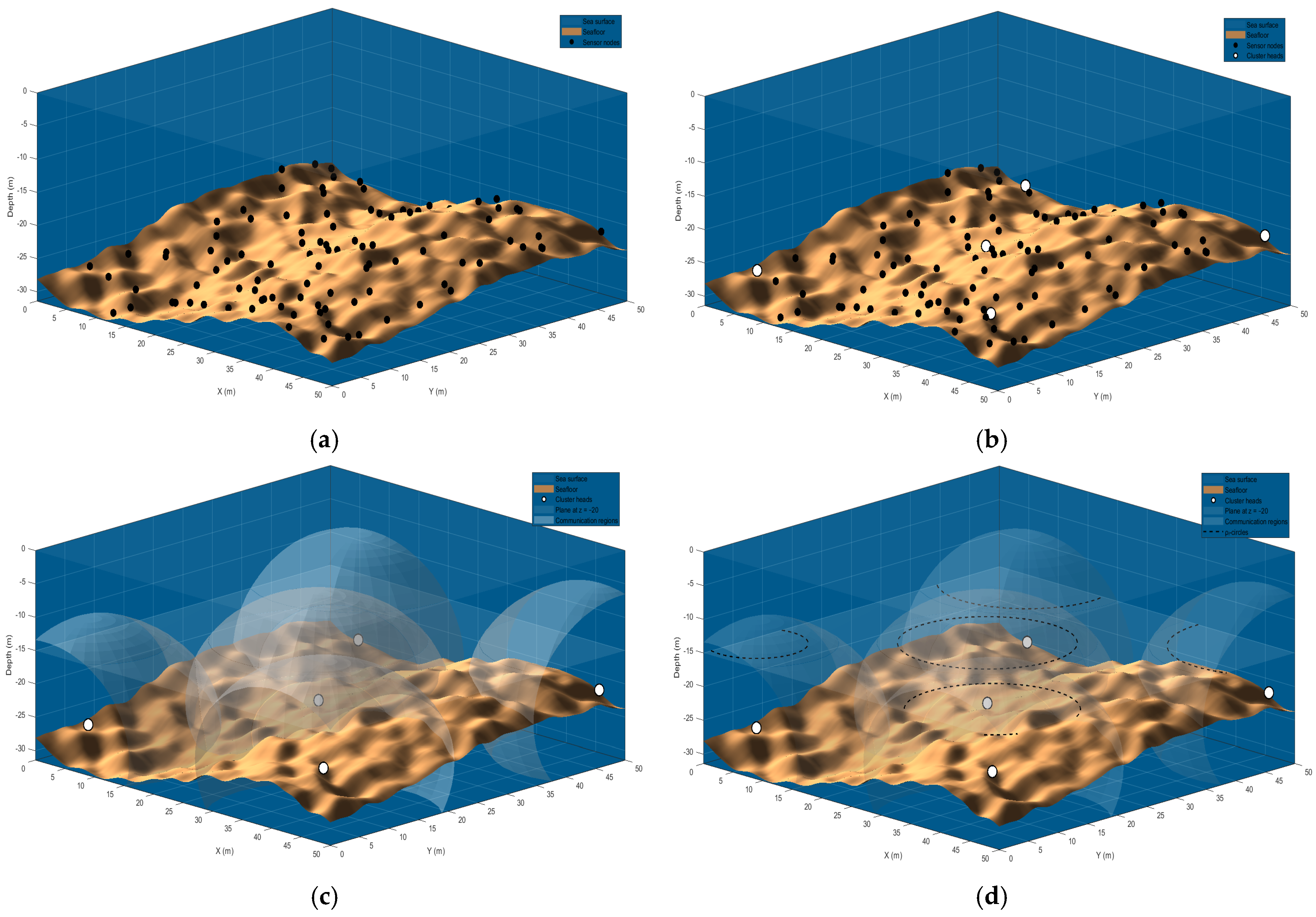
The simulation is conducted based on the UASN model illustrated in Figure 4. Figure 4a displays the target underwater environment, including the sensor nodes and the uneven seafloor. These sensor nodes are clustered using the k-medoids algorithm, and a CH is selected for each cluster, as shown in Figure 4b. Figure 4c depicts the communication sphere of radius $R_i$ for each CH, along with the horizontal plane at depth $z_d$, which defines the AUV’s operating level for data collection. In Figure 4d, each ${\mathcal{C}}_i$ is shown as a dashed circle representing the communication boundary of CH $i$ on the horizontal plane, centered at $(x_{{CH}_i},y_{{CH}_i},z_d)$ with radius ${\rho }_i$. The AUV can collect data from CH $i$ by reaching any point along the circumference of ${\mathcal{C}}_i$.

Figure 4. System overview showing: (a) sensor node distribution (black dots); (b) CH selection (white dots); (c) CH communication spheres intersecting the AUV’s horizontal operation plane; (d) the horizontal communication regions of each CH (dashed black circles).

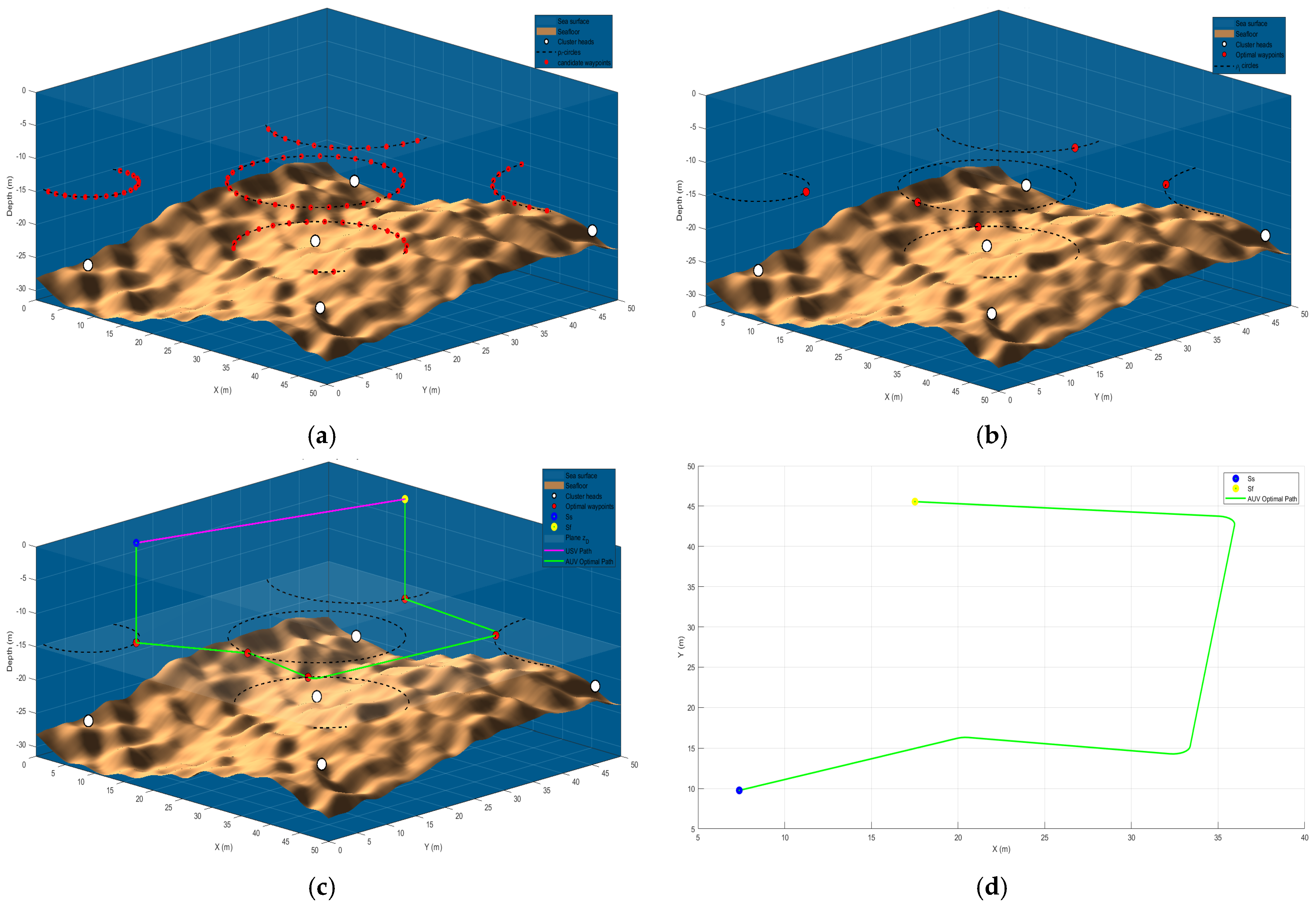
The task is to determine the AUV’s start and end points, along with a trajectory that visits exactly one point on the circumference of each ${\mathcal{C}}_i$, ensuring complete data collection while maximizing the total residual VoI upon returning to the USV on the surface. With all parameters defined, the proposed forward DP algorithm is applied to identify the optimal set of waypoints. A Dubins-like trajectory is then constructed to connect these waypoints.

The first step involves distributing a finite set of $L=30$ candidate waypoints uniformly along the circumference of each ${\mathcal{C}}_i$ (see Figure 5a). Any waypoints that fall outside the area of interest are excluded. The remaining waypoints constitute the state space for each CH, and the forward DP algorithm outlined in Algorithm 1 is employed to efficiently determine the optimal visiting sequence and associated waypoint selection, one point per ${\mathcal{C}}_i$, denoted by $({\mathsf{\Phi }}_{\mathrm{opt}},{\mathcal{P}}_{\mathrm{opt}})$, as illustrated in Figure 5b. The $x$ and $y$ coordinates of the first point in ${\mathcal{P}}_{\mathrm{opt}}$ are assigned to the USV’s starting point $S_s$, with its altitude set to $z=0$ to ensure placement on the sea surface. Likewise, the $x$ and $y$ coordinates of the final point in ${\mathcal{P}}_{\mathrm{opt}}$ define the USV’s endpoint $S_f$, with its altitude also set to $z=0$. Figure 5c illustrates the complete AUV trajectory, starting from $S_s$, marked with a blue dot, continuing through the selected waypoints in the optimal order, and ending at $S_f$, marked with a red dot, following the Dubins-like trajectory design described in Section 2.3.2. Figure 5d shows the 2D view of the final trajectory of the AUV.

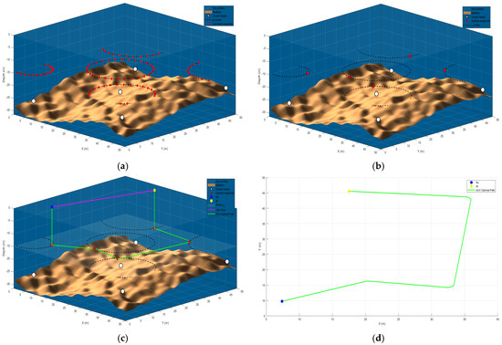
Figure 5. Implementation of the proposed method showing: (a) candidate waypoints distributed on each CH’s horizontal circle (red dots); (b) optimal waypoints selected by the forward DP algorithm (red dots); (c) final 3D trajectories of the AUV (green solid line) and the USV (magenta solid line) from the start point S_s (blue dot) to the end point S_f (yellow dot); (d) the final 2D trajectory of the AUV.

The proposed method demonstrated effectiveness by preserving approximately 66% of the total residual VoI across all CHs. The results further indicate that high-importance data decays more rapidly than medium-importance data. Nevertheless, the method retained around 64% of the high-importance information, which is considered satisfactory (see Table 1). This level of preservation supports the timely detection of abnormal events with minimal information loss, enabling rapid intervention in hazardous situations. However, the performance declines when the AUV operates over a larger area with widely dispersed CHs and a deeper surveillance plane, indicating that further improvements are required to maintain performance in more demanding environments.

Table 1. Final total residual VoI and corresponding preservation ratio.

$\mathit{i}$	$\mathbf{Initial} \mathbf{VoI} {\mathcal{V}}_{{\mathit{i}\mathit{n}\mathit{t}}_{\mathit{i}}}$	$\mathbf{Residual} \mathbf{VoI} {\mathit{V}}_{{\mathit{r}}_{\mathit{i}}}$	$\mathbf{Preserved} \mathbf{VoI} \mathbf{Ratio} \frac{{\mathit{V}}_{{\mathit{r}}_{\mathit{i}}}}{{\mathcal{V}}_{{\mathit{i}\mathit{n}\mathit{t}}_{\mathit{i}}}}$
1	0.8336	0.5507	66.1%
2	0.9626	0.6175	64.1%
3	0.7272	0.4921	67.7%
4	0.6432	0.4437	69%
5	0.9518	0.6121	64.3%
Total	4.1184	2.7161	65.9%

The following subsections present a performance analysis of the proposed method by comparing it against three strategies: straight-line trajectories, single-point CH selection, and traditional TSP-based path planning.

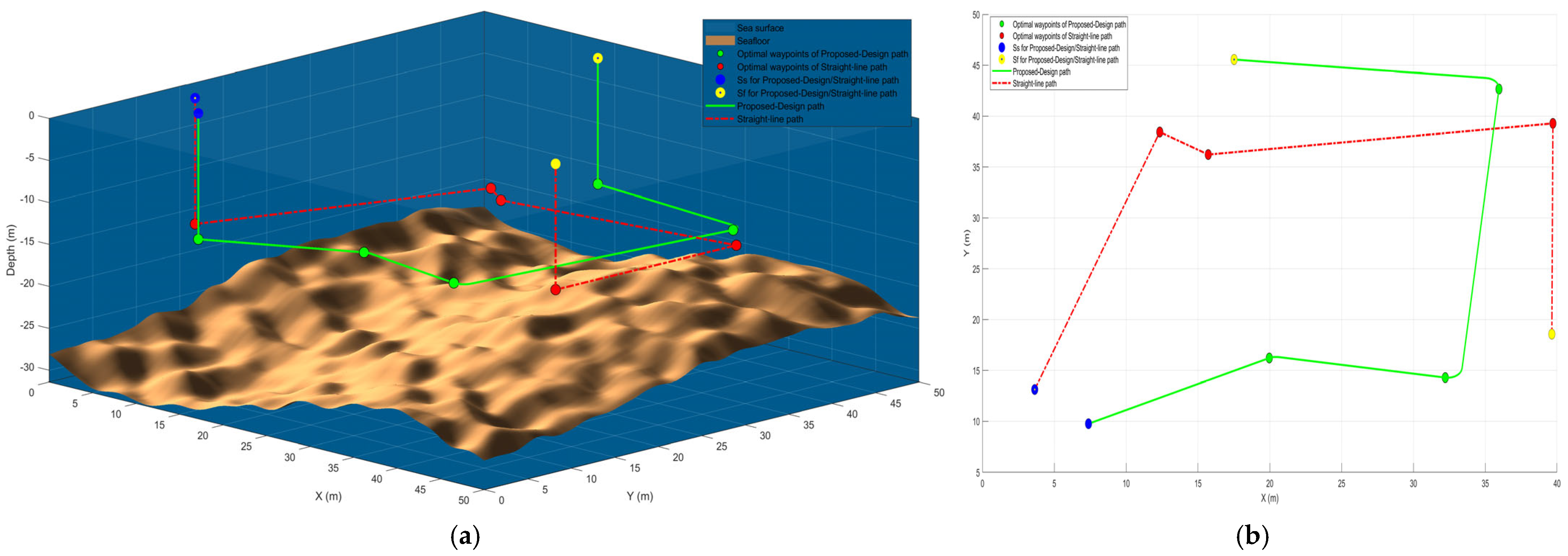
3.1. Straight-Line Trajectory Design Comparison

In the first comparison, we evaluate the impact of using Dubins-like trajectories proposed in this paper versus straight-line paths between waypoints. For each method, travel time is calculated based on the distance travelled and is used to guide the forward DP algorithm in selecting the optimal waypoints and their sequence. The straight-line strategy connects waypoints using Euclidean paths, assuming instantaneous heading changes. In contrast, our approach accounts for the AUV’s turning constraints, generating feasible trajectories that comply with its kinematic limitations.

As shown in Figure 6 and Table 2, the proposed method completes the mission 0.7% faster and preserves 0.3% more VoI, increasing the final VoI ratio from 65.75% to 65.95%. This improvement demonstrates that even small reductions in travel time can yield measurable gains due to the exponential decay of VoI. Moreover, the proposed trajectory avoids mismatches between planned and actual motion, enhancing overall mission efficiency.

Figure 6. Comparison of the proposed (green solid line) and the straight-line (red dash-dot line) path designs: (a) 3D trajectories and USV positions; (b) 2D x–y projection.

Table 2. Comparison of the proposed method with straight-line, single-point, and TSP-based designs.

	Proposed Method	Straight-Line Trajectory	Single-Point Design	TSP-Based Method
Total Residual VoI	2.7161	2.7080	2.0749	2.4568
Total time (s)	45.0167	45.3374	74.1794	55.8793
Preserved VoI Ratio	65.95%	65.75%	50.38%	59.65%

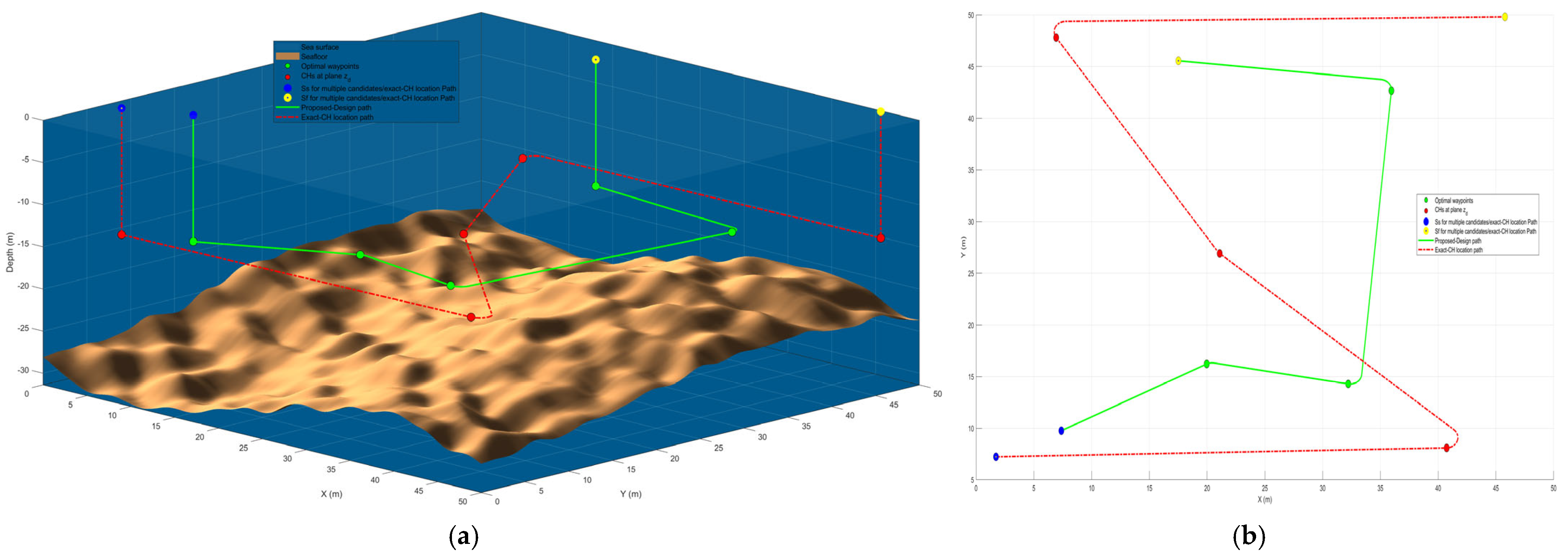
3.2. Single-Point Design Comparison

In this analysis, we investigate the impact of waypoint selection on overall mission performance. The proposed method selects optimal points from multiple candidates distributed along each CH’s horizontal communication circle and is compared with a simplified strategy that uses a single fixed point located directly above each CH. Both strategies use the same forward DP and path-planning framework but differ in waypoint flexibility.

The proposed method offers the forward DP algorithm a broader selection of candidate points, enabling it to identify routes with shorter travel times and improved VoI retention (see Figure 7). In contrast, the single-point approach constrains the AUV to less optimal trajectories, resulting in longer paths and increased VoI decay. The proposed method preserves 65.95% of the total VoI, while the fixed-point method retains only 50.38%, reflecting a 15.6% gain in VoI preservation driven by enhanced routing flexibility and reduced travel distance, which in turn leads to lower mission time and higher data preservation (refer to Table 2).

Figure 7. Comparison of the proposed (green solid line) and the single-point (red dash-dot line) designs: (a) 3D trajectories and USV positions; (b) 2D x–y projection.

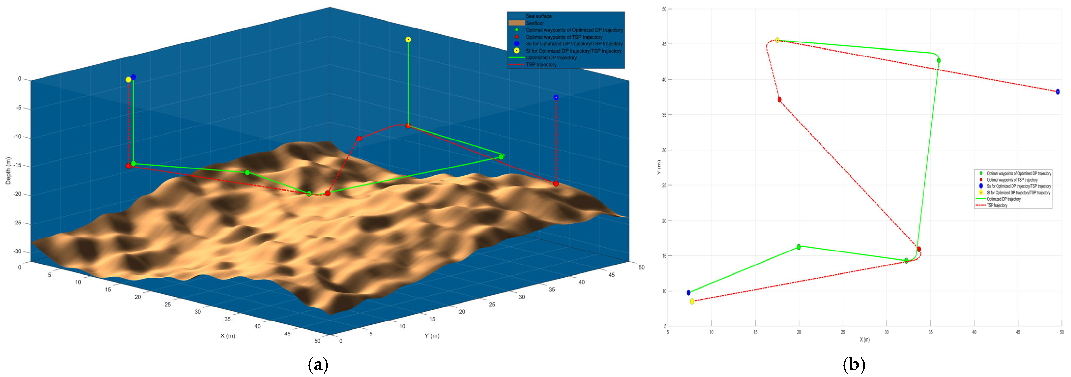
3.3. TSP-Based Method Comparison

In this section, we compare the proposed VoI-aware forward DP method with a conventional TSP-based approach. The TSP method solves the Euclidean Traveling Salesman Problem using the horizontal positions of CH centroids to minimize total travel distance. Once the TSP order is determined, a single waypoint per CH is selected, specifically, the one on its horizontal communication circle with the lowest travel time from the previous point. Both trajectories are executed using the proposed Dubins-like path design, and mission time and residual VoI are evaluated.

Figure 8 illustrates the resulting paths for both methods, highlighting the differences in waypoint selection and routing behavior. As shown in Table 2, the VoI-aware method outperforms the TSP-based approach by effectively prioritizing time-sensitive data. While the TSP method preserves 59.65% of the total VoI, the proposed method retains 65.95%, representing a 6% increase in VoI preservation. This improvement results from the forward DP method’s joint consideration of path feasibility, travel time, and data value, leading to more efficient and information-preserving trajectories. These findings demonstrate that distance-minimizing approaches alone do not necessarily yield the highest residual VoI.

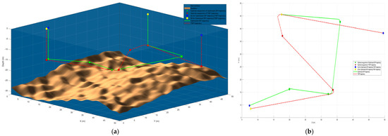
Figure 8. Comparison of the proposed forward DP (green solid line) and the TSP-based (red dash-dot line) methods: (a) 3D trajectories and USV positions; (b) 2D x–y projection.

4. Conclusions

This paper introduces a VoI-based trajectory planning approach for data collection in UASNs, where a single AUV collaborates with a USV to collect data from multiple CHs distributed over an uneven seafloor. The approach formulates an optimization problem aimed at maximizing the total residual VoI at mission completion, based on a VoI model that captures both data importance and timeliness. This problem is solved using a forward DP algorithm, which jointly optimizes the AUV’s trajectory and the USV’s start and end positions while satisfying the AUV’s kinematic constraints. Simulation results demonstrate promising performance in terms of total residual VoI and overall system efficiency compared to standard baselines. However, performance declined in larger and deeper environments with increased communication delays. These findings emphasize the need for enhanced system adaptability and motivate future extensions involving multi-AUV collaboration. Furthermore, accounting for sensing and transmission uncertainties is critical to accurately modeling real-world underwater conditions. Future work should also consider benchmarking the proposed method against state-of-the-art techniques to further validate its effectiveness.

References

- Liu, Z.; Meng, X.; Liu, Y.; Yang, Y.; Wang, Y. AUV-Aided Hybrid Data Collection Scheme Based on Value of Information for Internet of Underwater Things. IEEE Internet Things J. 2022, 9, 6944–6955. [Google Scholar] [CrossRef]
- Jahanbakht, M.; Xiang, W.; Hanzo, L.; Azghadi, M.R. Internet of Underwater Things and Big Marine Data Analytics—A Comprehensive Survey. IEEE Commun. Surv. Tutor. 2021, 23, 904–956. [Google Scholar] [CrossRef]
- Petritoli, E.; Leccese, F. Autonomous Underwater Glider: A Comprehensive Review. Drones 2025, 9, 21. [Google Scholar] [CrossRef]
- Greco, M.; Leccese, F.; Giarnetti, S.; De Francesco, E. A Multiporpouse Amphibious Rover (MAR) as Platform in Archaeological Field. In Proceedings of the 2022 IMEKO TC-4 International Conference on Metrology for Archaeology and Cultural Heritage, University of Calabria, Arcavacata, Italy, 19–21 October 2022; pp. 19–21. [Google Scholar]
- Tang, Y.; Jing, L.; Shi, W.; He, C. Dynamic Data Collection of AUV Based on Deep Reinforcement Learning. In Proceedings of the 2023 IEEE International Conference on Signal Processing, Communications and Computing (ICSPCC), Zhengzhou, China, 14–17 November 2023. [Google Scholar]
- Duan, R.; Du, J.; Jiang, C.; Ren, Y. Value-Based Hierarchical Information Collection for AUV-Enabled Internet of Underwater Things. IEEE Internet Things J. 2020, 7, 9870–9883. [Google Scholar] [CrossRef]
- Liu, Z.; Liang, Z.; Yuan, Y.; Chan, K.Y.; Guan, X. Energy-Efficient Data Collection Scheme Based on Value of Information in Underwater Acoustic Sensor Networks. IEEE Internet Things J. 2024, 11, 18255–18265. [Google Scholar] [CrossRef]
- Yan, J.; Yang, X.; Luo, X.; Chen, C. Energy-Efficient Data Collection over AUV-Assisted Underwater Acoustic Sensor Network. IEEE Syst. J. 2018, 12, 3519–3530. [Google Scholar] [CrossRef]
- Gjanci, P.; Petrioli, C.; Basagni, S.; Phillips, C.A.; Boloni, L.; Turgut, D. Path Finding for Maximum Value of Information in Multi-Modal Underwater Wireless Sensor Networks. IEEE Trans. Mob. Comput. 2018, 17, 404–418. [Google Scholar] [CrossRef]
- Li, Y.; Bai, J.; Chen, Y.; Lu, X.; Jing, P. High Value of Information Guided Data Enhancement for Heterogeneous Underwater Wireless Sensor Networks. J. Mar. Sci. Eng. 2023, 11, 1654. [Google Scholar] [CrossRef]
- Wang, C.; Shen, X.; Wang, H.; Xie, W.; Zhang, H.; Mei, H. Multi-Agent Reinforcement Learning-Based Routing Protocol for Underwater Wireless Sensor Networks With Value of Information. IEEE Sens. J. 2024, 24, 7042–7054. [Google Scholar] [CrossRef]
- Felemban, E.; Shaikh, F.K.; Qureshi, U.M.; Sheikh, A.A.; Qaisar, S.B. Underwater Sensor Network Applications: A Comprehensive Survey. Int. J. Distrib. Sens. Netw. 2015, 11, 896832. [Google Scholar] [CrossRef]
- Khan, M.T.R.; Ahmed, S.H.; Jembre, Y.Z.; Kim, D. An Energy-Efficient Data Collection Protocol with AUV Path Planning in the Internet of Underwater Things. J. Netw. Comput. Appl. 2019, 135, 20–31. [Google Scholar] [CrossRef]
- López-Barajas, S.; Sanz, P.J.; Marín-Prades, R.; Echagüe, J.; Realpe, S. Network Congestion Control Algorithm for Image Transmission—HRI and Visual Light Communications of an Autonomous Underwater Vehicle for Intervention. Future Internet 2025, 17, 10. [Google Scholar] [CrossRef]
- Hu, T.; Zhuo, X.; Tang, L.; Li, Z.; Lu, W.; Qu, F. Multi-AUV Collaborative Data Collection and Trajectory Planning in Integrated Sensing and Communication for Underwater Acoustic Networks. In Proceedings of the IEEE Vehicular Technology Conference, Singapore, 24–27 June 2024. [Google Scholar]
- Wang, J.; Liu, S.; Shi, W.; Han, G.; Yan, S. A Multi-AUV Collaborative Ocean Data Collection Method Based on LG-DQN and Data Value. IEEE Internet Things J. 2024, 11, 9086–9106. [Google Scholar] [CrossRef]
- Savkin, A.V.; Verma, S.C.; Anstee, S. Optimal Navigation of an Unmanned Surface Vehicle and an Autonomous Underwater Vehicle Collaborating for Reliable Acoustic Communication with Collision Avoidance. Drones 2022, 6, 27. [Google Scholar] [CrossRef]
- Françolin, C.C.; Rao, A.V.; Duarte, C.; Martel, G. Optimal Control of a Surface Vehicle to Improve Underwater Vehicle Network Connectivity. J. Aerosp. Comput. Inf. Commun. 2012, 9, 1–13. [Google Scholar] [CrossRef]
- Lv, Z.; Zhang, J.; Jin, J.; Liu, L. Link Strength for Unmanned Surface Vehicle’s Underwater Acoustic Communication. In Proceedings of the 2016 IEEE/OES China Ocean Acoustics (COA), Harbin, China, 9–11 January 2016; pp. 1–4. [Google Scholar]
- Eskandari, M.; Savkin, A.V. Kinodynamic Motion Model-Based MPC Path Planning and Localization for Autonomous AUV Teams in Deep Ocean Exploration. In Proceedings of the 33rd Mediterranean Conference on Control and Automation (MED’ 2025), Tangier, Morocco, 10–13 June 2025. [Google Scholar]
- Bertsekas, D. Dynamic Programming and Optimal Control: Volume I; Athena Scientific: Nashua, NH, USA, 2012; Volume 4, ISBN 1886529434. [Google Scholar]
- Zhao, L.; Bai, Y. Data Harvesting in Uncharted Waters: Interactive Learning Empowered Path Planning for USV-Assisted Maritime Data Collection under Fully Unknown Environments. Ocean Eng. 2023, 287, 115781. [Google Scholar] [CrossRef]
- Huang, M.; Zhang, K.; Zeng, Z.; Wang, T.; Liu, Y. An AUV-Assisted Data Gathering Scheme Based on Clustering and Matrix Completion for Smart Ocean. IEEE Internet Things J. 2020, 7, 9904–9918. [Google Scholar] [CrossRef]
- Huang, H.; Savkin, A.V.; Ni, W. Online UAV Trajectory Planning for Covert Video Surveillance of Mobile Targets. IEEE Trans. Autom. Sci. Eng. 2022, 19, 735–746. [Google Scholar] [CrossRef]
- Almutairi, A.; Carpent, X.; Furnell, S. Recommendation-Based Trust Evaluation Model for the Internet of Underwater Things. Future Internet 2024, 16, 346. [Google Scholar] [CrossRef]
- Kotis, K.; Stavrinos, S.; Kalloniatis, C. Review on Semantic Modeling and Simulation of Cybersecurity and Interoperability on the Internet of Underwater Things. Future Internet 2023, 15, 11. [Google Scholar] [CrossRef]
- Fu, X.; Kang, S. Deep Reinforcement Learning-Based Collaborative Data Collection in UAV-Assisted Underwater IoT. IEEE Sens. J. 2025, 25, 1611–1626. [Google Scholar] [CrossRef]
- Lai, R.; Zhang, B.; Gong, G.; Yuan, H.; Yang, J.; Zhang, J.; Zhou, M. Energy-Efficient Scheduling in UAV-Assisted Hierarchical Wireless Sensor Networks. IEEE Internet Things J. 2024, 11, 20194–20206. [Google Scholar] [CrossRef]
- Han, S.; Zhu, K.; Zhou, M.; Liu, X. Joint Deployment Optimization and Flight Trajectory Planning for UAV Assisted IoT Data Collection: A Bilevel Optimization Approach. IEEE Trans. Intell. Transp. Syst. 2022, 23, 21492–21504. [Google Scholar] [CrossRef]
- Cheng, M.; Guan, Q.; Ji, F.; Cheng, J.; Chen, W. Mobile Relaying-Based Reliable Data Collection in Underwater Acoustic Sensor Networks. IEEE Wirel. Commun. Lett. 2022, 11, 1795–1799. [Google Scholar] [CrossRef]
- Zhang, Z.; Xu, J.; Xie, G.; Wang, J.; Han, Z.; Ren, Y. Environment- and Energy-Aware AUV-Assisted Data Collection for the Internet of Underwater Things. IEEE Internet Things J. 2024, 11, 26406–26418. [Google Scholar] [CrossRef]
- Al-Bzoor, M.; Al-assem, E.; Alawneh, L.; Jararweh, Y. Autonomous Underwater Vehicles Support for Enhanced Performance in the Internet of Underwater Things. Trans. Emerg. Telecommun. Technol. 2021, 32, e4225. [Google Scholar] [CrossRef]
- Nandyala, C.S.; Cho, H.-S. AUV-Aided Isolated Sub-Network Prevention for Reliable Data Collection by Underwater Wireless Sensor Networks. Comput. Netw. 2025, 262, 111154. [Google Scholar] [CrossRef]
- Shi, W.; Tang, Y.; Jin, M.; Jing, L. An AUV-Assisted Data Gathering Scheme Based on Deep Reinforcement Learning for IoUT. J. Mar. Sci. Eng. 2023, 11, 2279. [Google Scholar] [CrossRef]
- Zhuo, X.; Wu, W.; Tang, L.; Qu, F.; Shen, X. Value of Information-Based Packet Scheduling Scheme for AUV-Assisted UASNs. IEEE Trans. Wirel. Commun. 2024, 23, 7172–7185. [Google Scholar] [CrossRef]
- Li, Y.; Sun, Y.; Ren, Q.; Li, S. AUV-Aided Data Collection Considering Adaptive Ocean Currents for Underwater Wireless Sensor Networks. China Commun. 2023, 20, 356–367. [Google Scholar] [CrossRef]
- Cheng, W.; Teymorian, A.Y.; Ma, L.; Cheng, X.; Lu, X.; Lu, Z. Underwater Localization in Sparse 3D Acoustic Sensor Networks. In Proceedings of the IEEE INFOCOM 2008—The 27th Conference on Computer Communications, Phoenix, AZ, USA, 13–18 April 2008; pp. 236–240. [Google Scholar]
- Santhiya, V.; Siron, N.; Simon, J. An Energy Efficient Multi-Level Clustering and Optimized Path Planning with Data Fusion (EEMLC-OPPDF) for Autonomous Underwater Vehicles (AUVs) in Underwater Wireless Sensor Networks. Int. J. Commun. Syst. 2025, 38, e6130. [Google Scholar] [CrossRef]
- Xia, N.; Luo, L.; Wang, Y.; Zhang, K.; Yang, J.; Wu, Q.; Yuan, C. Improved AP-Clustering-Based AUV-Aided Data Collection Method for UWSNs. Electronics 2023, 12, 3116. [Google Scholar] [CrossRef]
- Hart, P.E.; Nilsson, N.J.; Raphael, B. A Formal Basis for the Heuristic Determination of Minimum Cost Paths. IEEE Trans. Syst. Sci. Cybern. 1968, 4, 100–107. [Google Scholar] [CrossRef]
- Lawler, E.L.; Wood, D.E. Branch-and-Bound Methods: A Survey. Oper. Res. 1966, 14, 699–719. [Google Scholar] [CrossRef]
- Guang, X.; Liu, C.; Qu, W.; Qiu, T. A Joint Optimized Data Collection Algorithm Based on Dynamic Cluster-Head Selection and Value of Information in UWSNs. Veh. Commun. 2022, 38, 100530. [Google Scholar] [CrossRef]
- Khan, W.; Hua, W.; Anwar, M.S.; Alharbi, A.; Imran, M.; Khan, J.A. An Effective Data-Collection Scheme with AUV Path Planning in Underwater Wireless Sensor Networks. Wirel. Commun. Mob. Comput. 2022, 2022, 8154573. [Google Scholar] [CrossRef]
- Zhuo, X.; Liu, M.; Wei, Y.; Yu, G.; Qu, F.; Sun, R. AUV-Aided Energy-Efficient Data Collection in Underwater Acoustic Sensor Networks. IEEE Internet Things J. 2020, 7, 10010–10022. [Google Scholar] [CrossRef]
Disclaimer/Publisher’s Note: The statements, opinions and data contained in all publications are solely those of the individual author(s) and contributor(s) and not of MDPI and/or the editor(s). MDPI and/or the editor(s) disclaim responsibility for any injury to people or property resulting from any ideas, methods, instructions or products referred to in the content. |
© 2025 by the authors. Licensee MDPI, Basel, Switzerland. This article is an open access article distributed under the terms and conditions of the Creative Commons Attribution (CC BY) license (https://creativecommons.org/licenses/by/4.0/).