Topology-Aware Anchor Node Selection Optimization for Enhanced DV-Hop Localization in IoT

Abstract

Node localization is a critical challenge in Internet of Things (IoT) applications. The DV-Hop algorithm, which relies on hop counts for localization, assumes that network nodes are uniformly distributed. It estimates actual distances between nodes based on the number of hops. However, in practical IoT networks, node distribution is often non-uniform, leading to complex and irregular topologies that significantly reduce the localization accuracy of the original DV-Hop algorithm. To improve localization performance in non-uniform topologies, we propose an enhanced DV-Hop algorithm using Grey Wolf Optimization (GWO). First, the impact of non-uniform node distribution on hop count and average hop distance is analyzed. A binary Grey Wolf Optimization algorithm (BGWO) is then applied to develop an optimal anchor node selection strategy. This strategy eliminates anchor nodes with high estimation errors and selects a subset of high-quality anchors to improve the localization of unknown nodes. Second, in the multilateration stage, the traditional least square method is replaced by a continuous GWO algorithm to solve the distance equations with higher precision. Simulated experimental results show that the proposed GWO-enhanced DV-Hop algorithm significantly improves localization accuracy in non-uniform topologies.

1. Introduction

As a key component of next-generation information technology, the Internet of Things (IoT) connects physical objects to the Internet via information-sensing devices, forming a ubiquitous network architecture [1]. It bridges the physical and digital worlds, enabling seamless data exchange and communication among devices. This endows systems with intelligent capabilities, including identification, localization, tracking, monitoring, and management. Currently, IoT technology is widely applied across diverse domains—such as smart homes, intelligent transportation, industrial automation, and healthcare—playing a vital role in each [2]. Node localization plays a central role in the core technological framework of the IoT [3]. Accurate determination of IoT device locations is essential for implementing various IoT applications. As a foundational service for environmental sensing, data association, and decision-making optimization, node localization defines the spatial awareness capability of IoT systems. Its performance directly impacts the effectiveness and reliability of IoT applications.

Node localization techniques are generally classified into two categories based on their principles and implementation: range-based and range-free approaches [4]. Range-based methods estimate inter-node distances by measuring physical parameters such as signal strength, time delay, or angle. Representative techniques include Time of Arrival (TOA) [5], Time Difference of Arrival (TDOA) [6], Received Signal Strength Indicator (RSSI) [7], and Angle of Arrival (AOA) [8]. The TOA method calculates distance by measuring the time required for a signal to travel from the transmitting node to the receiving node. It provides high localization accuracy but demands strict time synchronization. The TDOA method determines location by measuring the arrival time differences at multiple receivers, effectively mitigating synchronization errors. The RSSI method estimates distance based on signal strength attenuation, but its accuracy is highly susceptible to environmental interference. The AOA method determines location by measuring the angle of signal arrival; however, it requires specialized hardware and is sensitive to interference in complex environments. In general, while range-based techniques offer higher accuracy, they involve greater complexity and higher implementation costs.

Range-free localization techniques do not require precise distance measurements or additional hardware. Instead, they estimate positions based on network topology or other contextual information. These methods are cost-effective but typically provide lower localization accuracy. Several range-free localization methods have been proposed, including DV-Hop [9], centroid localization [10], fingerprint-based localization [11], and the Approximate Point in Triangulation Test (APIT) [12]. The core principle of DV-Hop is to estimate unknown node positions by computing the number of hops and the average distance per hop. Centroid localization estimates the position of an unknown node as the geometric centre of nearby anchor nodes. Fingerprint-based localization constructs a fingerprint database by collecting signal characteristics at known reference points, and estimates the node position by matching current signal features to those in the database. The APIT algorithm estimates a node position by checking whether it lies within the triangle formed by three anchor nodes.

Compared to other range-free localization methods, the DV-Hop algorithm requires only inter-node communication to perform localization. This characteristic offers significant advantages in hardware requirements, implementation complexity, and network scalability, making DV-Hop a prominent method among range-free localization techniques. The DV-Hop algorithm consists of three main stages: hop count calculation, average hop distance estimation, and position determination of unknown nodes. First, through information flooding, all nodes acquire the positions of anchor nodes and their minimum hop counts to each one. Second, each anchor node calculates its average hop distance and broadcasts this information. Finally, each unknown node estimates its distance to each anchor based on the hop count and average hop distance, and then determines its position. The DV-Hop algorithm assumes a uniform distribution of nodes within the network. Under this assumption, hop counts can reliably approximate physical distances. However, in real-world IoT networks, node distributions are often non-uniform, leading to irregular and complex topologies. Such non-uniformity can cause significant errors in hop count estimation, which further result in inaccurate average hop distance calculations. The accumulation of these errors ultimately leads to a significant decline in the localization accuracy of DV-Hop under non-uniform topologies.

To enhance the localization performance of the original DV-Hop algorithm under non-uniform topologies, we integrate the Grey Wolf Optimization (GWO) algorithm [13] into the DV-Hop framework. Anchor nodes with large distance estimation errors are eliminated, and a subset of high-quality anchor nodes is selected to improve the localization accuracy of unknown nodes. The primary contributions of this study are summarized as follows:

(1)

The impact of non-uniform node distribution on hop count and average hop distance was analyzed. A binary Grey Wolf Optimization (BGWO) algorithm was employed to encode anchor nodes and establish an optimal anchor node selection mechanism.

(2)

During the multilateration stage, a continuous GWO algorithm was applied to replace the least squares method for position optimization, enhancing the accuracy of solving the distance equations.

(3)

The overall performance of the proposed algorithm was thoroughly evaluated through simulation experiments.

The organization of this paper is structured as follows: Section 2 reviews the related research background; Section 3 introduces the fundamental principles of the DV-Hop algorithm and discusses the impact of non-uniform node distribution on localization; Section 4 presents the GWO algorithm and its binary form; Section 5 provides a detailed explanation of the proposed improved algorithm; and Section 6 validates the localization performance of the proposed algorithm through simulations. Finally, Section 7 concludes this paper.

2. Related Works

Several review articles have been published on network node localization [14,15], which classify and introduce various localization algorithms and techniques proposed in recent years. This section focuses on papers related to the DV-Hop algorithm.

Shen et al. [16] proposed a correction strategy to optimize the average hop distance of anchor nodes, thereby improving the accuracy of the anchor node distances. By multiplying the unbiased estimated average hop distance by the hop count, the estimated distance between anchor nodes is obtained. The deviation between the estimated and actual distance is used as a correction factor to adjust the average hop distance of anchor nodes. Liu et al. [17] suggested that errors typically follow a Gaussian distribution and argued that using the minimum mean square error criterion, rather than unbiased estimation, is more suitable for calculating the average hop distance of anchor nodes. However, as sensor nodes are randomly deployed within the monitoring area, varying degrees of influence between anchor nodes should be expected. To address this, Chen et al. [18] used the hop count between anchor nodes as a weight and proposed a method for calculating the average hop distance of anchor nodes based on a weighted minimum mean square error criterion.

Song et al. [19] considered the impact of the average hop distance of anchor nodes across the network for distance estimation and proposed using the network-wide average hop distance of anchor nodes as the average hop distance for unknown nodes. However, in real-world scenarios, it is unlikely that all unknown nodes will share the same average hop distance. Abd EI Ghafour et al. [20] proposed a constraint strategy to limit the number of anchor nodes involved in the calculation, using the average hop distance of anchor nodes within the communication radius of the unknown node as the average hop distance of the unknown node. Furthermore, Chen et al. [21] analyzed the impact of anchor nodes on unknown nodes and assigned different weights to anchor nodes based on network connectivity and hop count. They proposed a weighted method to calculate the average hop distance of unknown nodes. Experimental results showed that the most accurate average hop distance for unknown nodes was achieved when 10% of the anchor nodes were involved in the calculation. Shi et al. [22] proposed a similar path search algorithm to obtain a multi-hop path between anchor nodes, identifying the optimal average hop distance by calibrating the average hop distance from the unknown node to each target anchor node. Ultimately, both the original DV-Hop algorithm and the aforementioned improved strategies use the product of the minimum hop count and average hop distance for distance estimation. In contrast, Sun et al. [23] proposed an accumulated hop distance method for distance estimation, where each anchor node uses the minimum mean square error criterion to obtain the average hop distance, and a weighted strategy is employed to calculate the average hop distance for unknown nodes. The node-to-node distance is then obtained by accumulating the average hop distances of the unknown nodes along the link.

Lv et al. [24] introduced a weighted least squares method to determine the position of unknown nodes, effectively reducing localization errors. To minimize error propagation in solving distance equations, Kumar et al. [25] proposed a localization algorithm called PERLA. This algorithm divides each distance equation by the one formed by the closest anchor node to the unknown node and uses the information generated during the solution to correct the coordinates of the unknown node. Tang et al. [26] designed an improved DV-Hop localization method based on Stephenson iteration. This method uses the localization result of the original DV-Hop as the initial value for the Stephenson iterative model and gradually converges to the true position of the unknown node through continuous iteration. Gui et al. [27] proposed the 3Anchor DV-Hop localization algorithm, which groups all anchor nodes into triplets and selects the best three from each group to locate the unknown node. Kaur et al. [28] argued that the closer an anchor node is to an unknown node, the more reliable the estimated distance between them becomes, and proposed using only the five closest anchor nodes for localization. However, different network parameters and topologies affect the number of anchor nodes involved in localization. In recent years, the rise of intelligent optimization algorithms has provided new approaches to optimizing DV-Hop localization. Scholars have applied various optimization algorithms to globally optimize the position of unknown nodes in the third stage of the original DV-Hop multilateration process. For example, improvements to DV-Hop based on Particle Swarm Optimization [29], Grey Wolf Optimization [30], Genetic Algorithm [31], and Artificial Bee Colony Optimization [32] have been proposed.

Although existing research strives to enhance the localization accuracy of the DV-Hop algorithm, it still faces challenges such as accuracy improvement bottlenecks and limitations in adaptability. This study aims to address critical shortcomings in current DV-Hop-based localization methods for IoT networks: First, the original DV-Hop algorithm is mainly applicable to scenarios with uniformly distributed nodes. In non-uniform networks, its performance deteriorates significantly, and the localization accuracy drops sharply. This study will conduct an in-depth analysis of the impact of non-uniform node distribution on the hop count between nodes and the average hop distance, pointing out that it disrupts the inherent relationship between the hop count and the physical distance. Second, the BGWO algorithm is introduced to establish an anchor node selection mechanism. By performing binary encoding on the participation states of anchor nodes and defining an optimization objective function based on localization error, BGWO can screen out a subset of dominant anchor nodes suitable for localizing unknown nodes in non-uniform networks. Only this subset is used for localization, effectively eliminating the interference from anchor nodes with unreliable estimated distances. Third, the GWO algorithm is adopted to directly minimize the distance error. This not only reduces the sensitivity to distance estimation errors but also avoids the dependence of the least squares algorithm on both estimation accuracy and initial iteration values, thus significantly improving the final localization accuracy. The collaborative innovation in the above three aspects provides a more effective localization method for non-uniform IoT networks.

3. Theoretical Backgrounds

3.1. Original DV-Hop Algorithm

DV-Hop is one of the most widely used localization algorithms due to its simplicity and the fact that it does not require ranging. Its implementation consists of the following three steps:

STEP 1: Calculation of the minimum hop count between sensor nodes

Each anchor node broadcasts data packets to the network in a flooding manner, which include the anchor node’s position and an initialized hop count of 0. When adjacent nodes receive the packet, they retain only the minimum hop count from the same anchor node and forward it, incremented by 1, to neighboring nodes. Once the flooding process is complete, all nodes will know the minimum hop count to each anchor node.

STEP 2: Estimating the distance between nodes

The anchor nodes calculate the average hop distance using an unbiased estimation method, as defined in Equation (1).

$$AH{S}_i={\displaystyle \frac{{\displaystyle \sum _{j\ne i}^{N_a}\sqrt{{\left(x_i-x_j\right)}^2+{\left(y_i-y_j\right)}^2}}}{{\displaystyle \sum _{j\ne i}^{N_a}{h}_{ij}}}}$$

(1)

where AHS_i denotes the average hop distance of anchor node i, N_a is the number of anchor nodes, (x_i, y_i) and (x_j, y_j) represent the position of anchor node i and j, respectively, and h_ij denotes the minimum hop count between anchor node i and j.

Once the average hop distance of anchor nodes is broadcast to the network, unknown nodes use the average hop distance of the first received anchor node as their own. The estimated distance between the unknown node and the anchor node is then calculated using Equation (2).

$$d_{ui}=AH{S}_u\times h_{ui}$$

(2)

where AHS_u denotes the average hop distance of the unknown node u, while h_ui and d_ui represent the minimum hop count and the estimated distance from the anchor node i to the unknown node u, respectively.

STEP 3: Calculation of the unknown node coordinates

Based on the distance estimates from the previous step and the known information of anchor nodes, the following distance equations are derived:

$$\left\{\begin{array}{c}\sqrt{{\left(x_u-x_1\right)}^2+{\left(y_u-y_1\right)}^2}=d_{u1}\\ \sqrt{{\left(x_u-x_2\right)}^2+{\left(y_u-y_2\right)}^2}=d_{u2}\\ ⋮\\ \sqrt{{\left(x_u-x_{N_a}\right)}^2+{\left(y_u-y_{N_a}\right)}^2}=d_{u2}\end{array}\right.$$

(3)

By successively subtracting the last equation from the first N_a − 1 equations, a linearized system of distance equations is derived:

$$\left\{\begin{array}{c}{x}_1^2+y_1^2-x_{N_a}^2-y_{N_a}^2-2x_u\left(x_1-x_{N_a}\right)-2y_u\left(y_1-y_{N_a}\right)=d_{u1}^2-d_{u{N}_a}^2\\ x_2^2+y_2^2-x_{N_a}^2-y_{N_a}^2-2x_u\left(x_2-x_{N_a}\right)-2y_u\left(y_2-y_{N_a}\right)=d_{u2}^2-d_{u{N}_a}^2\\ ⋮\\ x_{N_a-1}^2+y_{N_a-1}^2-x_{N_a}^2-y_{N_a}^2-2x_u\left(x_{N_a-1}-x_{N_a}\right)-2y_u\left(y_{N_a-1}-y_{N_a}\right)=d_{u\left(N_a-1\right)}^2-d_{u{N}_a}^2\end{array}\right.$$

(4)

The unknown node’s position can be determined by solving the above equation using the least squares method:

$$X={\left(A^{T}A\right)}^{-1}{A}^{T}B$$

(5)

where

$$A=2\left[\begin{array}{cc}\left(x_1-x_{N_a}\right)& \left(y_1-y_{N_a}\right)\\ \left(x_2-x_{N_a}\right)& \left(y_2-y_{N_a}\right)\\ ⋮& ⋮\\ \left(x_{N_a-1}-x_{N_a}\right)& \left(y_{N_a-1}-y_{N_a}\right)\end{array}\right]$$

(6)

$$B=\left[\begin{array}{c}{x}_1^2-x_{N_a}^2+y_1^2-y_{N_a}^2+d_{u{N}_a}^2-d_{u1}^2\\ x_2^2-x_{N_a}^2+y_2^2-y_{N_a}^2+d_{u{N}_a}^2-d_{u2}^2\\ ⋮\\ x_{N_a-1}^2-x_{N_a}^2+y_{N_a-1}^2-y_{N_a}^2+d_{u{N}_a}^2-d_{u\left(N_a-1\right)}^2\end{array}\right]$$

(7)

$$X=\left[\begin{array}{c}{x}_u\\ y_u\end{array}\right]$$

(8)

3.2. Effects of Non-Uniform Node Topology on the Localization Accuracy of the DV-Hop Algorithm

The original DV-Hop algorithm estimates the distance between unknown nodes and anchor nodes based on the average hop distance. In networks with uniformly distributed nodes, the average hop distance more accurately reflects the actual physical distance between nodes. In contrast, non-uniform topologies are often affected by obstacles in the monitoring area, which may prevent sensor deployment in specific regions. Obstacles may force nodes that could originally communicate within one or two hops to rely on multiple hops for connection. Changes in shortest routing paths disrupt the correlation between physical distance and hop count. Under such complex network conditions, the original DV-Hop algorithm fails to achieve the localization accuracy required for practical applications.

Although numerous enhancements to the original DV-Hop algorithm have been proposed, their performance often degrades significantly in the presence of irregular network topologies. Figure 1 illustrates the communication paths in a network with a non-uniform topology. It is evident that the hop count from node S to node A₁ is 3, whereas due to obstacles, the hop count from node S to node A₂ increases to 6. However, the actual distance d₁ between node S and node A₁ is evidently greater than d₂, the distance between node S and node A₂. In uniformly distributed networks, it is generally assumed that a higher hop count indicates a greater physical distance. This assumption, however, does not hold in non-uniform topologies, where the correlation between hop count and physical distance is often disrupted. As a result, based on the principles of the original DV-Hop algorithm, the estimated distances between certain unknown nodes and anchor nodes may become unreliable.

4. Grey Wolf Optimization Algorithm and Its Binary Variant

4.1. Continuous Version of the Grey Wolf Optimization Algorithm

In recent years, swarm intelligence optimization algorithms have rapidly emerged, providing effective solutions to a wide range of engineering optimization problems. Among these, continuous GWO, proposed by Mirjalili et al. [13], stands out as a classical algorithm and has attracted considerable attention from researchers. The algorithm is inspired by the strict social hierarchy and cooperative hunting strategies of grey wolves. To simulate hunting and social behavior, the population is categorized into four roles: α, β, δ, and ω wolves. The α wolf serves as the highest-ranking leader, β wolves assist in decision-making, δ wolves follow α and β wolves, and the remaining are classified as ω wolves. During the optimization process, the positions of ω wolves are iteratively updated under the guidance of the top three wolves (α, β, and δ).

During the hunting phase, grey wolves track and encircle their prey, a behavior mathematically defined as follows:

$$D=\left|C\cdot X_p(t)-X(t)\right|$$

(9)

$$X(t+1)=X_p(t)-A\cdot D$$

(10)

where t denotes the current iteration number, while X and X_p represent the position vectors of a grey wolf and the prey, respectively. D represents the distance between a grey wolf and the prey. The coefficient vectors A and C are defined as follows:

$$A=2\cdot a\cdot r_1-a$$

(11)

$$C=2\cdot r_2$$

(12)

$$a=2-2\cdot t/T_{\max }$$

(13)

where r₁ and r₂ are random vectors uniformly distributed in the range [0, 1]. The parameter a is a convergence factor that decreases linearly from 2 to 0 as the number of iterations increases. T_max denotes the maximum number of iterations.

Once the prey is located, the α wolf leads the β and δ wolves to encircle it. This tracking behavior is mathematically defined as follows:

$$D_i=\left|C\cdot X_i-X\right|;i=\alpha ,\beta ,\delta$$

(14)

where X denotes the current position of the grey wolf. C represents a random vector, while Xₐ, Xᵦ, and X_δ indicate the positions of the α, β, and δ wolves, respectively. Dₐ, Dᵦ, and D_δ denote the distances between the α, β, and δ wolves and other individuals.

$$X_j=X_i-A\cdot D_i;i=\alpha ,\beta ,\delta ;j=1,2,3$$

(15)

$$X(t+1)={\displaystyle \frac{X_1+X_2+X_3}{3}}$$

(16)

where X₁, X₂, and X₃ denote the step size and direction of the ω wolf as it moves toward the α, β, and δ wolves, respectively. The final position of the ω wolf is then determined by Equation (16).

The GWO algorithm has advantages such as a small number of control parameters and good robustness [33]. Since its proposal, the GWO algorithm has been successfully applied to solve numerous complex optimization problems. Conducting a theoretical analysis of the convergence of the GWO algorithm contributes to a deeper understanding of its working principle and performance. Reference [34] analyzed the convergence of the GWO algorithm by constructing a mathematical model of a Markov chain based on the convergence criteria of the stochastic search algorithm. We successfully proved that the GWO algorithm can achieve global convergence with probability 1 by means of the martingale convergence theorem [35].

4.2. Binary Grey Wolf Optimization Algorithm

In the GWO algorithm, each grey wolf’s position can be any point in the solution space, which is commonly used to solve continuous problems. For certain problems, such as feature selection, the solutions are restricted to the binary set {0, 1}. To bridge the gap between continuous and binary spaces, Emary et al. [36] proposed the BGWO algorithm to address combinatorial optimization problems in discrete spaces. In the binary space, the grey wolf’s position is updated by replacing values with “0” or “1”. The positions of α, β, and δ are initialized using Equation (17):

$$X_i=\left[x_k\right],x_k=\left\{\begin{array}{c}0\hspace{1em}rand<0.5\hfill \\ 1\hspace{1em}\hspace{1em} else\hfill \end{array}\right.;i=\alpha ,\beta ,\delta ;k=1,2,\cdots ,n$$

(17)

where n represents the dimension of the optimization problem.

In the binary space, the grey wolf’s position is updated between “0” and “1” using a conversion function at each iteration. The conversion function is as follows:

$$S(X_i(t))={\displaystyle \frac{1}{1+\exp (\left|X_i(t)\right|)}};i=\alpha ,\beta ,\delta$$

(18)

$$X_i(t)=\left[x_k\right],x_k=\left\{\begin{array}{c}0\hspace{1em}S(X_i(t))<rand\hfill \\ 1\hspace{1em}\hspace{1em}\hspace{1em} else\hfill \end{array}\right.;i=\alpha ,\beta ,\delta ;k=1,2,\cdots ,n$$

(19)

By applying Equations (18) and (19), continuous problems are transformed into discrete ones. The position of the grey wolf is then updated based on the conversion values from the function using the following equation:

$$X(t+1)=\left\{\begin{array}{c}1\hspace{1em}S({\displaystyle \frac{X_{\alpha }(t)+X_{\beta }(t)+X_{\delta }(t)}{3}})\ge rand\hfill \\ 0\hspace{1em}\hspace{1em}\hspace{1em}\hspace{1em}\hspace{1em}\hspace{1em} else\hfill \end{array}\right.$$

(20)

5. Proposed Algorithm

5.1. Anchor Node Selection Mechanism Using BGWO

In continuous optimization problems, the grey wolf’s position can take any value within a defined range. However, in BGWO for discrete problems, the position vector can only take values of “0” or “1”. To develop an anchor node selection mechanism using BGWO, the grey wolf’s position values must be determined based on the characteristics of DV-Hop localization. Anchor nodes either participate in the localization of unknown nodes or do not. Thus, the position vector of the optimal grey wolf in BGWO indicates whether an anchor node is involved in localization. Assume there are M grey wolves and N_a anchor nodes in the network. The position vector of the i-th grey wolf is represented as follows: X_i = (x_i1, x_i2, …, x_iNa), where the dimensionality of the vector corresponds to the total number of anchor nodes. The position vector is initialized using Equation (17) and updated based on Equation (19) during each iteration. If x_ik = 1, it indicates that the k-th anchor node is a suitable anchor node for localization. If x_ik = 0, the k-th anchor node does not participate in the localization process. To better illustrate the anchor node selection mechanism, consider a non-uniformly distributed network with six anchor nodes. If the grey wolf’s position vector is [0, 1, 1, 0, 1, 0], it means that localization of the unknown node will use only the second, third, and fifth anchor nodes, while the others will not participate.

After determining the values of the grey wolf’s position vector, the coordinates of the corresponding anchor nodes, which have a value of “1”, can be calculated using the least squares method. Additionally, due to the limited available information in the network during the localization phase, only the position coordinates of the anchor nodes and the estimated distances from unknown nodes to anchor nodes are known. Thus, when using BGWO to select anchor nodes, Equation (21) serves as the fitness function to evaluate the quality of the grey wolf’s position.

$$fitness\_bgwo(X)={\displaystyle \frac{{\displaystyle \sum _{i=1}^{N_a}{(\sqrt{{(x_i-x_u)}^2+{(y_i-y_u)}^2}-d_{ui})}^2}}{N_a\cdot R}}$$

(21)

where (x_u, y_u) represents the estimated coordinates of the unknown node u, obtained using the corresponding anchor nodes with a value of “1” in the position vector. (x_i, y_i) represents the position coordinates of the anchor node i, and R is the communication radius of nodes.

The fitness function, corresponding to Equation (21), exhibits high sensitivity to the quality of anchor nodes involved in the calculation. When lower-quality anchor nodes participate in localization, significant deviations arise between the estimated distances from the unknown node u to these anchors and the actual distances. This subsequently leads to a larger fitness function value resulting from the least squares localization solution. Conversely, when all participating anchor nodes are of high quality, the deviations between the estimated and actual distances from the unknown node u to anchor nodes are smaller. In this case, the least squares localization solution yields a relatively smaller fitness function value. Consequently, based on this characteristic, this paper selects Equation (21) as the fitness function and employs the BGWO algorithm for optimization. The position vector of the grey wolf obtained through this algorithm’s optimization determines the final set of anchor nodes participating in the calculation.

5.2. Localization Optimization Using GWO

To enhance the accuracy of the original DV-Hop algorithm, GWO is employed during the localization phase to replace the least squares method for determining the unknown node’s position. Using the proposed anchor node selection mechanism, the grey wolf’s position vector with the minimum fitness value selects the corresponding anchor nodes (with a value of “1”) to participate in the localization, while those with a value of “0” are excluded. In the GWO algorithm, to solve the distance equations formed by the dominant anchor nodes, the position vector of each grey wolf is represented as [x, y], indicating the potential coordinates of the unknown node. The initial position coordinates of each grey wolf are randomly generated within the range [0, 100] and updated in each iteration using Equation (16).

During global optimization with GWO, Equation (22) is used as the fitness function to evaluate the quality of the grey wolf’s position. The smaller the value of fitness_gwo, the closer the grey wolf’s position to the true location of the unknown node. Once the predefined number of iterations is reached, the position of the grey wolf with the minimum fitness value is selected as the final estimated coordinates of the unknown node.

$$fitness\_gwo(X)={\displaystyle \frac{{\displaystyle \sum _{i=1}^K{(\sqrt{{(x_i-x_u)}^2+{(y_i-y_u)}^2}-d_{ui})}^2}}{K\cdot R}}$$

(22)

where K represents the number of dominant anchor nodes selected using the BGWO anchor node selection mechanism.

Due to the inevitable errors in the estimated distances from unknown nodes to anchor nodes, when using the least squares method for multilateration localization, according to Equation (7), the accuracy of the least squares solution depends on the estimation accuracy of d_uNa. If the estimation deviation of d_uNa is large, the deviation generated by the least squares calculation will also increase accordingly. In contrast, when using the GWO algorithm for multilateration localization, Equation (22) is used as the fitness function value. This algorithm directly minimizes the distance measurement error. The minimum value obtained from the algorithm optimization is the localization coordinate of the unknown node. This method not only reduces the sensitivity to distance estimation errors but also avoids the dependence on the initial iteration values, demonstrating unique advantages.

5.3. The Complete Procedure of the Improved Localization Algorithm Is Outlined as Follows

To address the issue of poor distance estimation accuracy caused by non-uniform node distribution in the IoT, the BGWO algorithm is incorporated into the localization phase for anchor node selection. Each anchor node is initially encoded using “0–1” coding. Anchor nodes with large distance estimation errors are excluded based on changes in the fitness values of the grey wolves. In the multilateration localization phase, only the anchor nodes selected by BGWO are used for localizing unknown nodes, and the GWO algorithm replaces the least squares method for estimating the unknown node’s position. While retaining the advantages of the original DV-Hop algorithm, its third phase is optimized and enhanced. The complete flowchart of the improved DV-Hop localization algorithm is presented in Figure 2.

6. Simulation and Results Analysis

6.1. Network Simulation Model

The simulation area is 100 m × 100 m, consisting of 100 nodes, 30 of which are anchor nodes. All nodes have a communication radius of 20 m, and the degree of channel irregularity (DOI) is set to 0.05 [37]. Both the BGWO and GWO algorithms are set to a maximum of 50 iterations, with 30 grey wolves, and their initial positions are randomly generated. The relevant simulation parameters are provided in

Table 1. Simulation parameters.

Parameter	Value
Node deployment	random
Monitoring region	100 m × 100 m
Sensor nodes	100
Anchor nodes	30
Communication range	20 m
Channel Irregularity Degree (DOI)	0.05
Number of iterations in the GWO	50
Population size of the GWO	30

. In comparison to networks with uniformly distributed nodes, IoT networks with non-uniform topologies exhibit several rectangular or hole-like areas where node deployment is not possible. The simulation experiments are based on three classic non-uniform network topologies: C-type, O-type, and W-type, illustrated in Figure 3.

6.2. Performance Evaluation Criteria

(1)

The normalized localization error for a single unknown node

$$LocErro{r}_u={\displaystyle \frac{\sqrt{{(x_u^{true}-x_u^{est})}^2+{(y_u^{true}-y_u^{est})}^2}}{R}}$$

(23)

where ($x_u^{true}$, $y_u^{true}$) represents the actual coordinates of the unknown node u, while ($x_u^{est}$, $y_u^{est}$) denotes its estimated coordinates obtained through the localization algorithm. LocError_u refers to the normalized localization error of the unknown node u.

(2)

Computation of the network-wide normalized average localization error

$$ANLE={\displaystyle \frac{{\displaystyle \sum _{u=1}^{N_u}\sqrt{{(x_u^{true}-x_u^{est})}^2+{(y_u^{true}-y_u^{est})}^2}}}{R\cdot N_u}}$$

(24)

where N_u denotes the number of unknown nodes, and ANLE refers to the normalized average localization error of the network. A higher value indicates poorer performance of the localization algorithm.

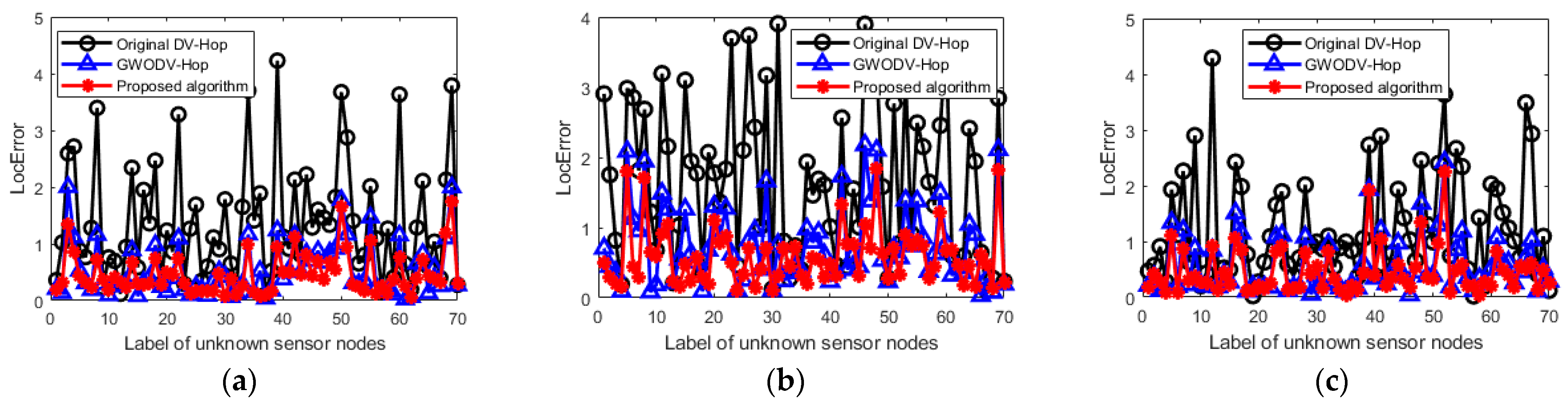
6.3. Comparison of Localization Errors in Non-Uniform Network Topologies

To evaluate the effectiveness of the proposed algorithm, the original DV-Hop [38] and GWODV-Hop algorithms [39] were chosen for comparison. Both the DV-Hop and GWODV-Hop algorithms utilize all anchor nodes for localization, with GWODV-Hop substituting the least squares method with the GWO algorithm to solve the distance equations. In contrast, the proposed algorithm uses the BGWO algorithm to exclude anchor nodes with large distance errors, relying only on a subset of dominant anchor nodes and the GWO algorithm for localization of unknown nodes.

(1)

Normalized localization error of unknown nodes

Figure 4 illustrates the localization errors of unknown nodes for the three comparison algorithms under non-uniform network topologies. As shown in the figure, the original DV-Hop algorithm exhibits the worst localization accuracy in non-uniform networks, while both GWODV-Hop and the proposed algorithm demonstrate significant improvements in accuracy. In C-type and O-type networks, the accuracy of all three localization algorithms fluctuates to varying degrees. Although GWODV-Hop achieves higher accuracy for certain individual unknown nodes, the overall localization error of the proposed algorithm is significantly lower than that of GWODV-Hop. In the W-type network, the normalized localization error of the proposed algorithm fluctuates around 0.5, while some localization results of unknown nodes in GWODV-Hop exhibit larger deviations. The results confirm that network obstacles significantly affect the localization performance of the original DV-Hop algorithm. By utilizing the global optimization capability of intelligent optimization algorithms, localization errors can be minimized. Additionally, applying the proposed algorithm to eliminate anchor nodes heavily influenced by obstacles can further enhance the localization accuracy of unknown nodes.

(2)

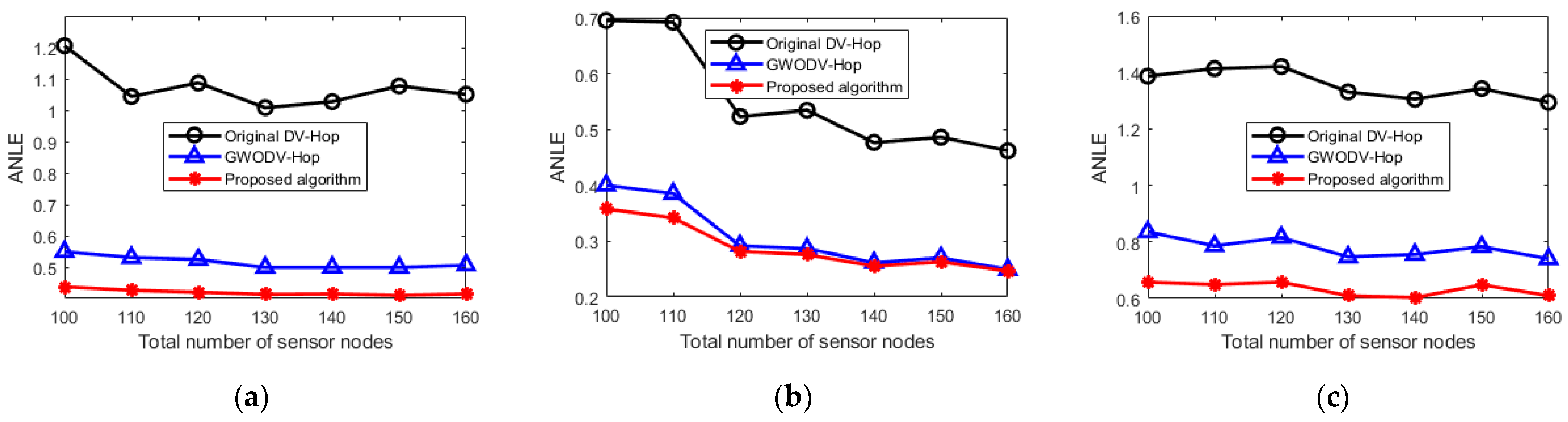
Impact of total number of nodes on localization performance

Under the simulation conditions outlined in Section 6.1, the total number of sensor nodes in the network was gradually increased from 100 to 160, while other parameters remained unchanged. Figure 5 illustrates the normalized localization errors of each algorithm across the three network topologies. As seen in Figure 5, as the total number of nodes increases, the localization errors of the original DV-Hop, GWODV-Hop, and the proposed algorithm decrease, with the proposed algorithm consistently yielding the lowest error. Specifically, in the O-type network, the increase in the total number of nodes has the most significant impact on localization accuracy, with the rate of error reduction being notably faster than in the C-type and W-type networks. Furthermore, the performance gap between the proposed algorithm and GWODV-Hop is more pronounced in the C-type and W-type networks, but the difference in localization errors gradually narrows in the O-type network.

Table 2. Average normalized localization error for each algorithm with 100–160 nodes.

Algorithm	Original DV-Hop			GWODV-Hop			Proposed Scheme
	C-Type	O-Type	W-type	C-Type	O-Type	W-Type	C-Type	O-Type	W-Type
Average value	1.0712	0.5526	1.3565	0.5154	0.3063	0.7808	0.4195	0.2888	0.6339

presents the average normalized localization errors of the original DV-Hop, GWODV-Hop, and the proposed algorithm across the three network topologies for total node counts ranging from 100 to 160. The experimental results confirm that the localization accuracy of all algorithms is sensitive to changes in the total number of nodes, with the proposed algorithm achieving the best performance across all three network topologies.

(3)

Impact of different number of anchor nodes on localization performance

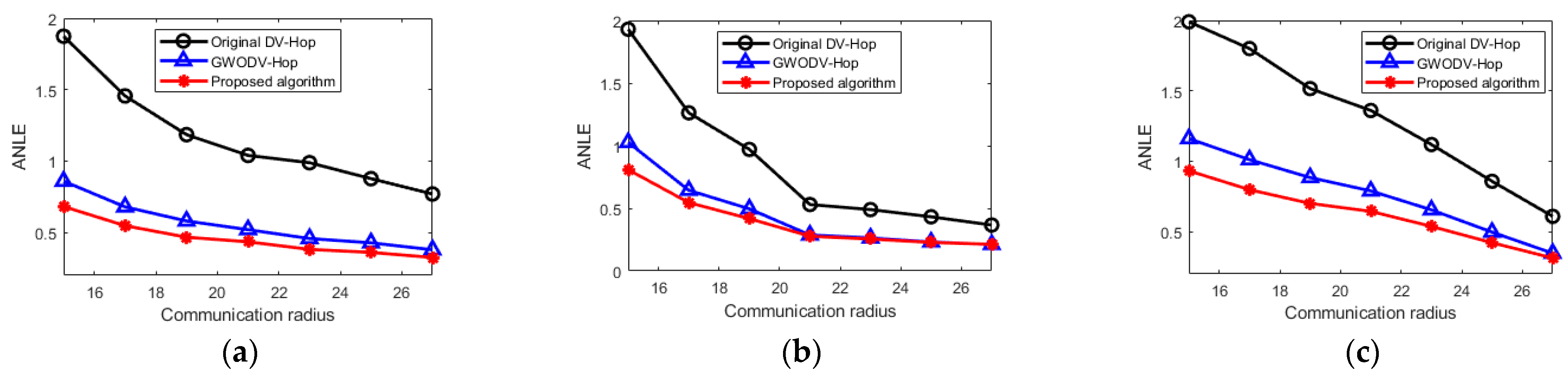
In a network with 100 nodes and a communication radius of 20 m, the proportion of anchor nodes was progressively increased. The performance of each localization algorithm in three network topologies is presented in Figure 6. The figure shows that the original DV-Hop algorithm exhibits the highest localization error, with significant fluctuations in the O-type network, distinguishing it from the other two algorithms. The proposed algorithm and GWODV-Hop show slight fluctuations in localization errors, but the proposed algorithm consistently achieves superior accuracy.

Table 3. Average normalized error of each algorithm with 15–45 anchor nodes.

Algorithm	Original DV-Hop			GWODV-Hop			Proposed Scheme
	C-Type	O-Type	W-Type	C-Type	O-Type	W-Type	C-Type	O-Type	W-Type
Average value	1.1665	0.7373	1.4176	0.5561	0.3950	0.8214	0.4554	0.3603	0.6742

shows the average normalized localization errors for the original DV-Hop, GWODV-Hop, and the proposed algorithm as the number of anchor nodes increases from 15 to 45 in the three network topologies. The average data indicate that all three algorithms perform best in the O-type network, while their performance is comparatively poorer in the W-type network. The simulation results indicate that as the proportion of anchor nodes increases, the proposed algorithm’s anchor node selection mechanism significantly enhances the localization accuracy of the original DV-Hop.

(4)

The impact of different communication radius on localization performance

Figure 7 illustrates the variation in localization errors for each localization algorithm as the communication radius increases, with 100 nodes and 30% anchor nodes across three network topologies. Overall, both the GWODV-Hop and proposed algorithms exhibit significantly lower localization errors than the original DV-Hop, with their errors being similar. In the C-type network, the localization errors of all three algorithms gradually decrease with increasing communication radius. In the O-type networks, the error trends for all three algorithms are similar, initially decreasing rapidly and then stabilizing. In the W-shaped network, the proposed algorithm slightly outperforms GWODV-Hop. The average localization errors of the three algorithms within the communication radius range are shown in

Table 4. Average normalized error of each algorithm within communication radius 15–27 m.

Algorithm	Original DV-Hop			GWODV-Hop			Proposed Algorithm
	C-Type	O-Type	W-Type	C-Type	O-Type	W-Type	C-Type	O-Type	W-Type
Average value	1.1699	0.8545	1.3217	0.5577	0.4512	0.7635	0.4571	0.3920	0.6210

. The experimental results suggest that as the communication radius increases, the proposed algorithm outperforms others in localization across the three network topologies.

6.4. Comparison of Localization Stability Under Non-Uniform Network Topology

Figure 8 presents the cumulative distribution functions of normalized localization errors for the original DV-Hop, GWODV-Hop, and proposed algorithms across three network topologies. A steeper curve indicates stronger stability of the algorithm. The curves for the proposed algorithm and GWODV-Hop rise more rapidly than those of the original DV-Hop. In the O-type network, however, their increase rates are relatively similar. The results indicate that localization stability is highest in the O-type network and lowest in the W-type network for all three algorithms. Furthermore, Figure 8 clearly shows that the curve for the proposed algorithm is always steeper than those for the original DV-Hop and GWODV-Hop across all three networks, indicating superior localization stability.

6.5. Node Localization Time Analysis

Table 5. Average localization time for a single unknown node (unit: ms).

Algorithm	Running Times (s)
Original DV-Hop	8.46
GWODV-Hop	27.38
Proposed algorithm	40.71

presents the average time required to locate a single unknown node for the original DV-Hop, GWODV-Hop, and the proposed algorithm in non-uniform network topologies. The original DV-Hop algorithm benefits from its simple implementation, giving it an advantage in localization time. Both GWODV-Hop and the proposed algorithm use GWO to determine the unknown node’s position, with the convergence speed of GWO affecting the localization time. The processing time required by the GWODV-Hop algorithm is 223.6% more than that of the original DV-Hop algorithm. The increase in computational overhead is mainly because, during the multilateration stage, the GWO algorithm is adopted instead of the least squares method to determine the positions of unknown nodes. This results in additional calculations of the fitness function and updates of the population in the GWO algorithm. The proposed algorithm, compared to GWODV-Hop, filters anchor nodes using BGWO prior to localization, thus resulting in the processing time of the proposed algorithm being approximately 48.7% longer than that of the GWODV-Hop algorithm. As a result, the localization time of the proposed algorithm and GWODV-Hop is increased to a certain extent compared to the original DV-Hop. Although the localization time of the proposed algorithm is extended, the enhanced localization accuracy demonstrates significant application potential for the proposed method in industrial monitoring scenarios with stringent precision requirements. The time data presented in Table 5 were obtained under the stopping criterion of reaching the maximum iteration count. For IoT devices with real-time constraints, an early stopping criterion can be established. The iterative process may be terminated prematurely when the change in the fitness function value over multiple consecutive iterations falls below a predefined threshold, indicating that the proposed algorithm has converged. However, in terms of hardware complexity, the proposed algorithm does not require significant modification to the existing IoT node hardware. Nevertheless, it does demand slightly more memory to store the intermediate data generated during the BGWO-based anchor node selection process. Compared with the overall memory capacity of modern IoT nodes, this additional memory requirement is relatively small. Despite this, the proposed algorithm consistently shows superior localization accuracy and stability across various simulation scenarios with non-uniform network topologies.

7. Conclusions

This paper proposes an enhanced DV-Hop node localization method based on the Grey Wolf Optimization algorithm to mitigate the reduced localization accuracy caused by the non-uniform distribution of nodes in IoT networks. The impact of non-uniform node distribution on hop count and average hop distance is analyzed, and a binary GWO-based anchor node selection mechanism is designed to filter superior anchor nodes, enabling precise localization of unknown nodes. During the multilateration phase, the continuous GWO algorithm replaces the least squares method for localization optimization, greatly enhancing the accuracy of the distance equations. Simulation results demonstrate that the improved algorithm effectively mitigates the cumulative effects of hop count and average hop distance errors caused by non-uniform node distribution, leading to significant improvements in localization accuracy in non-uniform topologies. This approach offers an efficient and precise solution for node localization in IoT networks.

References

1. Čolaković, A.; Hadžialić, M. Internet of Things (IoT): A review of enabling technologies, challenges, and open research issues. Comput. Netw. 2018, 144, 17–39. [Google Scholar] [CrossRef]
2. Perwej, Y.; Haq, K.; Parwej, F.; Mohamed Hassan, M.M. The internet of things (IoT) and its application domains. Int. J. Comput. Appl. 2019, 182, 36–49. [Google Scholar] [CrossRef]
3. Ghorpade, S.; Zennaro, M.; Chaudhari, B. Survey of localization for internet of things nodes: Approaches, challenges and open issues. Future Internet 2021, 13, 210. [Google Scholar] [CrossRef]
4. Singh, P.; Mittal, N.; Salgotra, R. Comparison of range-based versus range-free WSNs localization using adaptive SSA algorithm. Wirel. Netw. 2022, 28, 1625–1647. [Google Scholar] [CrossRef]
5. Chen, H.; Liu, B.; Huang, P.; Liang, J.; Gu, Y. Mobility-assisted node localization based on TOA measurements without time synchronization in wireless sensor networks. Mob. Netw. Appl. 2012, 17, 90–99. [Google Scholar] [CrossRef]
6. Ennasr, O.; Tan, X. Time-difference-of-arrival (TDOA)-based distributed target localization by a robotic network. IEEE Trans. Control Netw. Syst. 2020, 7, 1416–1427. [Google Scholar] [CrossRef]
7. Wang, W.; Liu, X.; Li, M.; Wang, Z.H.; Wang, C. Optimizing node localization in wireless sensor networks based on received signal strength indicator. IEEE Access 2019, 7, 73880–73889. [Google Scholar] [CrossRef]
8. Xu, J.; Ma, M.; Law, C.L. Cooperative angle-of-arrival position localization. Measurement 2015, 59, 302–313. [Google Scholar] [CrossRef]
9. Chen, T.; Hou, S.; Sun, L. An enhanced DV-Hop positioning scheme based on spring model and reliable beacon node set. Comput. Netw. 2022, 209, 108926. [Google Scholar] [CrossRef]
10. Wang, J.; Urriza, P.; Han, Y.; Cabric, D. Weighted centroid localization algorithm: Theoretical analysis and distributed implementation. IEEE Trans. Wirel. Commun. 2011, 10, 3403–3413. [Google Scholar] [CrossRef]
11. Sun, K.; Sun, L.; Chen, T. Indoor Positioning Model Based on Principal Component Extraction of Support Vector Regression. In Proceedings of the 2024 36th Chinese Control and Decision Conference (CCDC), Xi’an, China, 25–27 May 2024; IEEE: Piscataway, NJ, USA, 2024; pp. 2667–2672. [Google Scholar]
12. Liu, J.; Wang, Z.; Yao, M.; Qiu, Z.H. VN-APIT: Virtual nodes-based range-free APIT localization scheme for WSN. Wirel. Netw. 2016, 22, 867–878. [Google Scholar] [CrossRef]
13. Mirjalili, S.; Mirjalili, S.M.; Lewis, A. Grey wolf optimizer. Adv. Eng. Softw. 2014, 69, 46–61. [Google Scholar] [CrossRef]
14. Cheng, L.; Wu, C.; Zhang, Y.; Wu, H.; Li, M.; Maple, C. A survey of localization in wireless sensor network. Int. J. Distrib. Sens. Netw. 2012, 8, 962523. [Google Scholar] [CrossRef]
15. Kuriakose, J.; Joshi, S.; Vikram Raju, R.; Aravind, K. A review on localization in wireless sensor networks. In Advances in Signal Processing and Intelligent Recognition Systems, Proceedings of the first International Symposium on Signal Processing and Intelligent Recognition Systems (SIRS-2014), Trivandrum, India, 13–15 March 2014; Springer: Berlin/Heidelberg, Germany, 2014; pp. 599–610. [Google Scholar]
16. Shen, S.; Yang, K.; Qian, K.; She, Y.; Wang, W. On Improved DV-Hop Localization Algorithm for Accurate Node Localization in Wireless Sensor Networks. Chin. J. Electron. 2019, 28, 658–666. [Google Scholar] [CrossRef]
17. Liu, C.H.; Zhang, L. Optimization of Localization Accuracy of Wireless Sensor Network Based on DV-Hop Algorithm. Laser Optoelectron. Prog. 2021, 58, 2228007. [Google Scholar]
18. Chen, T.; Sun, L.; Wang, Z.; Wang, Y.; Zhao, Z.; Zhao, P. An enhanced nonlinear iterative localization algorithm for DV_Hop with uniform calculation criterion. Ad Hoc Netw. 2021, 111, 102327. [Google Scholar] [CrossRef]
19. Song, G.; Tam, D. Two Novel DV-Hop Localization Algorithms for Randomly Deployed Wireless Sensor Networks. Int. J. Distrib. Sens. Netw. 2015, 11, 187670. [Google Scholar] [CrossRef]
20. Abd EIGhafour, M.G.; Kamel, S.H.; Abouelseoud, Y. Improved DV-Hop based on Squirrel search algorithm for localization in wireless sensor networks. Wirel. Netw. 2021, 27, 2743–2759. [Google Scholar] [CrossRef]
21. Chen, T.; Sun, L. A Connectivity Weighting DV_Hop Localization Algorithm Using Modified Artificial Bee Colony Optimization. J. Sens. 2019, 2019, 1464513. [Google Scholar] [CrossRef]
22. Shi, Q.; Xu, Q.; Zhang, J. Improvement for DV-Hop Based on Distance Correcting and Grey Wolf Optimization Algorithm. Chin. J. Sens. Actuators 2019, 32, 1549–1555. [Google Scholar]
23. Sun, B.; Wei, S.; Li, D. Localization Algorithm for Wireless Sensor Network Based on Accumulated Hop Distance and Calibration Factor. Instrum. Tech. Sens. 2019, 2, 109–113. [Google Scholar]
24. Lv, J.; Long, M.; Yin, K. DV-Hop Location Algorithm Based on Weighted Least Squares Optimization. Chin. J. Sens. Actuators 2020, 33, 450–455. [Google Scholar]
25. Kumar, S.; Lobiyal, D.K. Power efficient range-free localization algorithm for wireless sensor networks. Wirel. Netw. 2014, 20, 681–694. [Google Scholar] [CrossRef]
26. Tang, D.; Wang, Y.; Ma, X. Sensor node localization mechanism based on improved DV-Hop algorithm. J. Jilin Univ. (Eng. Technol. Ed.) 2022, 52, 3015–3021. [Google Scholar]
27. Gui, L.; Val, T.; Wei, A.; Dalce, R. Improvement of range-free localization technology by a novel DV-hop protocol in wireless sensor networks. Ad Hoc Netw. 2015, 24, 55–73. [Google Scholar] [CrossRef]
28. Kaur, A.; Kumar, P.; Gupta, G.P. Improving DV-Hop-Based Localization Algorithms in Wireless Sensor Networks by Considering Only Closest Anchors. Int. J. Inf. Secur. Priv. 2020, 14, 1–15. [Google Scholar] [CrossRef]
29. Chen, X.; Zhang, B. 3D DV–hop localisation scheme based on particle swarm optimisation in wireless sensor networks. Int. J. Sens. Netw. 2014, 16, 100–105. [Google Scholar] [CrossRef]
30. Xu, Z. Wireless Sensor Network Localization Incorporating Gray Wolf Optimization and DVHop Algorithm. IEEE Access 2024, 12, 168594–168606. [Google Scholar] [CrossRef]
31. Sun, H.; Li, H.; Meng, Z.; Dong, W. An improvement of dv-hop localization algorithm based on improved adaptive genetic algorithm for wireless sensor networks. Wirel. Pers. Commun. 2023, 130, 2149–2173. [Google Scholar] [CrossRef]
32. Zhang, W.; Yang, X.; Song, Q. Improved DV-Hop algorithm based on artificial bee colony. Int. J. Control Autom. 2015, 8, 135–144. [Google Scholar] [CrossRef]
33. Zhang, X.; Wang, X. Comprehensive review of grey wolf optimization algorithm. Comput. Sci. 2019, 46, 30–38. [Google Scholar]
34. Zhang, M.; Long, D.; Wang, X.; Yang, J. Research on convergence of grey wolf optimization algorithm based on Markov chain. Acta Anat. Sin. 2020, 48, 1587–1595. [Google Scholar]
35. Sun, L.; Feng, B.; Chen, T. Global convergence analysis of grey wolf optimization algorithm based on martingale theory. Control Decis. 2022, 37, 2839–2848. [Google Scholar]
36. Emary, E.; Zawbaa, H.M.; Hassanien, A.E. Binary grey wolf optimization approaches for feature selection. Neurocomputing 2016, 172, 371–381. [Google Scholar] [CrossRef]
37. Liu, X.; Han, F.; Ji, W.; Liu, Y.; Xie, Y. A Novel Range-Free Localization Scheme Based on Anchor Pairs Condition Decision in Wireless Sensor Networks. IEEE Trans. Commun. 2020, 68, 7882–7895. [Google Scholar] [CrossRef]
38. Niculescu, D.; Nath, B. DV Based Positioning in Ad Hoc Networks. Telecommun. Syst. 2003, 22, 267–280. [Google Scholar] [CrossRef]
39. Sun, B.; Wei, S. DV-Hop Localization Algorithm Based on Grey Wolf Optimization Algorithm with Adaptive Adjutment Strategy. Comput. Sci. 2019, 46, 77–82. [Google Scholar]
Figure 1. Communication paths between nodes in a non-uniformly distributed topology network.
Futureinternet 17 00253 g001
Figure 2. Flowchart of the proposed localization algorithm.
Futureinternet 17 00253 g002
Figure 3. Three representative non-uniform network topologies. (a) C-type network; (b) O-type network; (c) W-type network.
Futureinternet 17 00253 g003
Figure 4. Normalized localization error of unknown nodes. (a) C-type network; (b) O-type network; (c) W-type network.
Futureinternet 17 00253 g004
Figure 5. Localization accuracy under different total numbers of nodes. (a) C-type network; (b) O-type network; (c) W-type network.
Futureinternet 17 00253 g005
Figure 6. Localization accuracy under different number of beacons. (a) C-type network; (b) O-type network; (c) W-type network.
Futureinternet 17 00253 g006
Figure 7. Localization accuracy under different communication radii. (a) C-type network; (b) O-type network; (c) W-type network.
Futureinternet 17 00253 g007
Figure 8. Stability of each localization algorithm under non-uniform network topologies. (a) C-type network; (b) O-type network; (c) W-type network.
Futureinternet 17 00253 g008