Signal Preprocessing for Enhanced IoT Device Identification Using Support Vector Machine

Abstract

Device identification based on radio frequency fingerprinting is widely used to improve the security of Internet of Things systems. However, noise and acquisition inconsistencies in raw radio frequency signals can affect the effectiveness of classification, identification and authentication algorithms used to distinguish Bluetooth devices. This study investigates how the RF signal preprocessing techniques affect the performance of a support vector machine classifier based on radio frequency fingerprinting. Four options derived from an RF signal preprocessing technique are evaluated, each of which is applied to the raw radio frequency signals in an attempt to improve the consistency between signals emitted by the same Bluetooth device. Experiments conducted on raw Bluetooth signals from twentyfour smartphone radios from two public databases of RF signals show that selecting an appropriate RF signal preprocessing approach can significantly improve the effectiveness of a support vector machine classifier-based algorithm used to discriminate Bluetooth devices.

1. Introduction

Signal preprocessing is critical for reliable data analysis, especially in applications such as healthcare [1,2], financial forecasting [3,4], and security [5,6], where high-quality data or signals are essential for accurate decision-making. This process addresses the inherent complexity of data quality deficiencies by employing techniques such as inconsistency removal and missing value imputation, which can improve the classification accuracy by up to 80% [7]. The global data preparation tools market, valued at USD 4.86 billion in 2022, is projected to grow at a CAGR of 16.1% between 2023 and 2030, reflecting its increasing adoption in industries that rely on data-driven insights [8].

One prominent area where the impact of data preprocessing is particularly evident is in the analysis of radio frequency fingerprints (RFFs). These are unique and inherent signatures produced by radio frequency electronic devices during wireless communication and offer immense potential for applications in wireless security, IoT device authentication, and spectrum monitoring [9,10]. Ensuring the reliability of RFF data requires robust signal preprocessing techniques to mitigate challenges such as noise, acquisition inconsistencies, and information loss, which can otherwise compromise the effectiveness of identification and classification systems [11,12]. For this purpose, five data preprocessing paradigms have been identified: data cleaning, data reduction, data transformation, data partitioning, and data scaling [13]. These paradigms are used to improve the quality of raw data, ensuring accurate and efficient analytical results in RFF analysis.

Recent advances in data preprocessing and classification techniques have significantly improved the accuracy of various machine learning applications but also revealed notable challenges. For instance, task-oriented filtering and homomorphic processing combined with SHAP-based classifiers achieved 97.3% accuracy for vehicle-to-everything (V2X) devices. However, these methods have limited generalization [14]. Similarly, Wavelet Transform and differential spectrum analysis using autoencoder-based schemes achieved 98.84% accuracy for LTE device categories, but computational complexity and noise sensitivity restrict scalability [15]. Deep learning models for the RFF identification demonstrate over 90% accuracy under controlled conditions but are susceptible to signal variability in real-world deployments [16]. In energy analysis, semi-supervised learning and data augmentation techniques improve reliability but are constrained by the need for large, labeled datasets and consistent signal preprocessing [13]. Random railings enhancement (RRE) improves minority class representation in unbalanced datasets, but its performance is sensitive to the underrepresentation of certain classes [17]. Supervised contrastive learning-based CNNs (CNN-SCL) achieve 92.68% accuracy with limited samples, although the results depend heavily on the quality of feature encoding [18]. Neural synchronization, which combines signal processing with data-driven learning, improves open-set discrimination. However, its success depends on the quality of the signal preprocessing for generalization [19]. The application of Gramian angular fields (1D/2D) paired with channel-selectable CNNs achieves up to 99.26% accuracy at high SNR, but its effectiveness requires clean signal segments [20]. Similarly, channel-independent spectrograms coupled with deep metric learning offer scalability and robust RFF identification for LoRa devices, although computational overhead remains a limitation for real-time applications. Virtual database generators, such as RiFyFi-VDG, simulate hardware impairments to achieve an average of 94% accuracy; however, they may introduce biases that hinder generalization to real-world scenarios [21]. In another approach, the probability density function (PDF) of noise signals from Bluetooth RF signals was compared using Jensen–Shannon divergence (JSD) for device identification. This statistical method achieved 99.5% accuracy on a dataset of 2400 signals from 16 devices, which were sampled at 5 Gsps [22]. Signal preprocessing steps included bandpass filtering and amplitude scaling to standardize the signals. Despite its high effectiveness in controlled environments, this approach relies on steady-state noise and remains susceptible to misclassification in noisy, real-world conditions. Short-time Fourier transform (STFT) and carrier frequency offset (CFO) compensation have been used for signal preprocessing LoRa signals, achieving 93.85% accuracy for legitimate device classification and 90.23% for rogue device detection using a KNN classifier [23]. However, this method showed limitations in scalability and robustness, with performance degrading under open-set scenarios with high noise levels and increased dataset openness. In contrast, a federated learning (FL) framework has been proposed to construct RFF datasets for IoT, UAVs, and Bluetooth devices. This framework uses logistic regression to improve generalization under privacy constraints. Although FL addresses data heterogeneity and privacy challenges, it introduces complexity in synchronization and is highly dependent on data quality and distribution [24].

Building on the growing body of research highlighting the critical role of signal preprocessing in RFF analysis, this paper evaluates the impact of a signal preprocessing technique on the effectiveness of an SVM-based classifier used to discriminate Bluetooth devices based on their RF fingerprints. This study demonstrates that an RF signal preprocessing technique applied with four approaches implies a low processing time, but it improves the effectiveness of an SVM-based classifier. Specifically, four variants of a scaling signal preprocessing technique are implemented to address problems such as noise and signal variability, which often negatively affect the performance of classification systems when applied in real-world situations. These signal preprocessing variants are normalized raw signal, mean-normalized raw signal, max-normalized raw signal, and min-normalized raw signal. Therefore, this study presents a systematic analysis to know how different variants of the same parameterized technique of RF signal preprocessing can affect the effectiveness of a classification algorithm used to discriminate Bluetooth devices. This approach demonstrates that the intermediate step between acquiring the RF signals and either defining the RF fingerprints of Bluetooth devices or estimating the radio-in-signal traces is critical to the effectiveness of an identification or discrimination strategy. For the purpose of this study, a Bluetooth signal dataset was used, which contains 150 RF signals from each of 16 smartphones, representing eight different models with two smartphones by model. This Bluetooth signal dataset was constructed from the RF signal dataset created by Uzundurukan et al. [25]. In addition, the SVM-based classifier was used considering that it is widely used in fingerprinting research [25].

The paper is divided into five sections. Section 2 provides a comprehensive overview of the RF signal dataset consisting of Bluetooth signals from multiple devices. It provides the definition and characteristics of these signals and details the RF signal preprocessing possibilities derived from a scaling technique. In addition, this section describes the configuration of the SVM-based classifier used to distinguish Bluetooth devices, including the selection of the kernel, and the experimental setup for training and testing. Section 3 presents the effect of each RF signal preprocessing option on the effectiveness of the SVM-based classifier, using confusion matrices and accuracy metrics in the evaluation. This section shows how different RF signal preprocessing options affect the effectiveness of the classifier considering various device classes. Section 4 provides a comprehensive analysis of the results, emphasizing the strengths and limitations of each signal preprocessing option. It explains the causes of misclassifications and evaluates the trade-off between improving accuracy and preserving computational efficiency, comparing the findings with other state-of-the-art works. Furthermore, this section highlights potential areas for improvement, such as increasing the model’s robustness to noise and its ability to generalize effectively across different datasets. Finally, Section 5 summarizes the key findings, emphasizing the importance of RF signal preprocessing in improving the effectiveness of the RFF-based device identification. It discusses the broader implications for IoT security and suggests future research directions, including advanced feature extraction, real-world validation, and the exploration of alternative machine learning models to further improve classification performance.

2. Materials and Methods

2.1. Dataset Description

The RF signal dataset used in this work was extracted from the RF signal dataset created by Uzundurukan et al. [25]. They captured RF signals from 27 smartphones, representing six different manufacturers. For each Bluetooth, they captured 150 RF signals, for a total of 4050 signal recordings. They acquired RF signals under controlled conditions to minimize external interference and to ensure high data quality and consistency. The Uzundurukan dataset includes RF signals recorded at 5 Gsps, 10 Gsps, and 20 Gsps using a TDS7404 oscilloscope manufactured by Tektronix, Inc., located in Oregon, USA. In addition, lower-frequency signals were acquired at 250 Msps using a modular RF front-end system connected to the oscilloscope. To complement the experimental evaluation, we also considered the publicly available dataset by Rusins et al. [26], which focuses on Bluetooth and Bluetooth Low Energy (BLE) communications from wearable devices. This dataset captures the complete communication cycle—including advertising, pairing, data exchange, and disconnection—under highly controlled conditions within an anechoic chamber to ensure RF isolation. A total of 32 wearable Bluetooth devices were used, including smartwatches, fitness bands, and headsets, with each device recorded in both paired and unpaired modes. The recordings were conducted using a USRP X310 software-defined radio (SDR) with a CBX-120 daughterboard, at a sample rate of 100 MHz and saved as complex64 I/Q samples. Each recording lasts approximately 10 to 30 s and includes metadata with precise timing of Bluetooth events. The dataset also includes baseline noise recordings and was specifically designed to support RF fingerprinting, Bluetooth protocol analysis, and cybersecurity research. For this work, a total of 24 device-class radios were selected: 16 smartphones from the Uzundurukan dataset and 8 additional wearable Bluetooth devices from the Rusins dataset. The 16 smartphones were organized into 8 twin pairs, each representing a different brand or model. Each device in a twin pair was treated as a distinct class, even though both belonged to the same model. For example, as shown in

Table 1. Smartphone classes and models in the case study.

Class	Device Name
1	Amazfit Band 5
2	Apple Watch SE
3	Fitbit Charge 5
4	Fitbit Versa 4
5	Garmin Instinct Crossover
6	Garmin Instinct SQ
7	Apple Watch Series 8
8	iPhone 5 - 1
9	iPhone 5 - 2
10	iPhone 6 - 1
11	iPhone 6 - 2
12	iPhone 5s - 1
13	iPhone 5s - 2
14	iPhone 6s - 1
15	iPhone 6s - 2
16	LG G4 - 1
17	LG G4 - 2
18	Samsung Note3 - 1
19	Samsung Note3 - 2
20	Samsung S5 - 1
21	Samsung S5 - 2
22	Samsung Galaxy S20 FE
23	Sony Xperia M5 - 1
24	Sony Xperia M5 - 2

, Class 1 corresponds to “iPhone 5 - 1”, while Class 2 corresponds to its twin, “iPhone 5 - 2”. This approach of categorization was consistently applied to all other smartphone pairs. Similarly, the four wearable devices from the Rusins dataset—each belonging to a different brand and device type—were also assigned to separate classes, resulting in a total of 24 unique classes across both datasets.

Understanding the distinctions between these classes is critical for evaluating RFF performance, as subtle variations between twin devices test the robustness of the classification algorithm. These class distinctions are further explored in the next section, where the definition and characteristics of raw Bluetooth signals are discussed in detail. This provides the foundation for analyzing how these signals can be used to uniquely identify devices within and across classes.

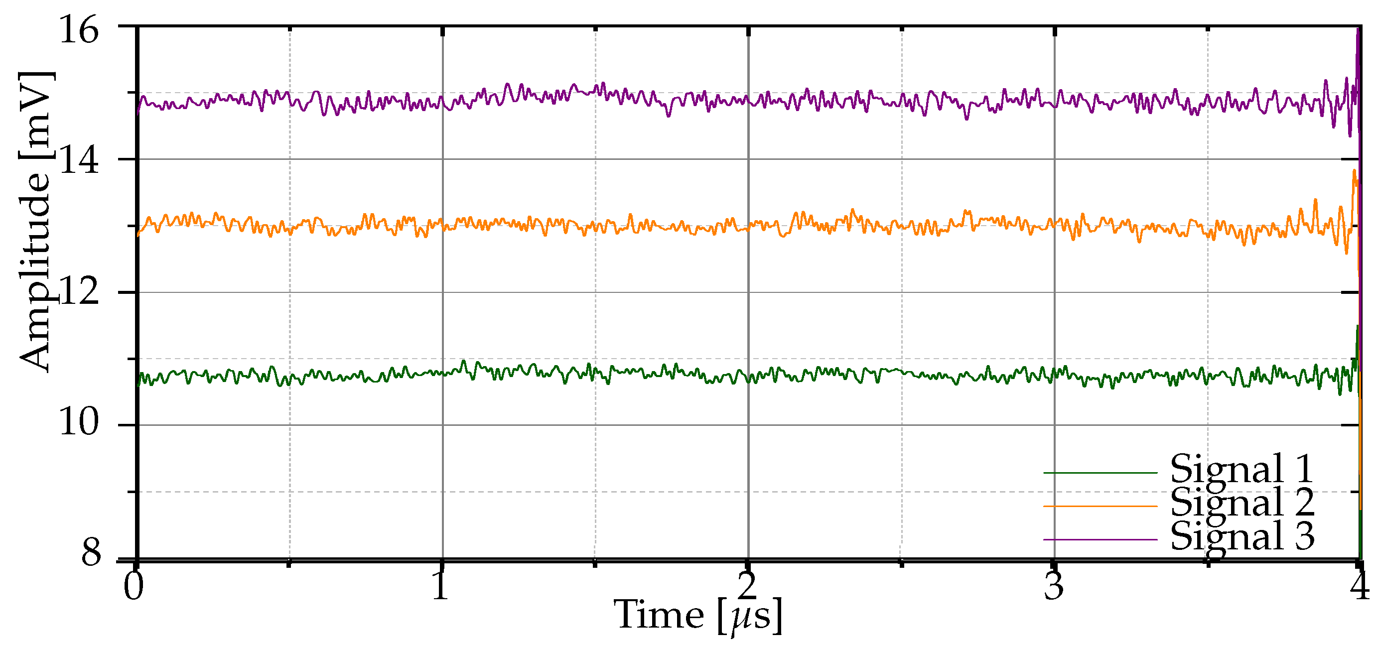
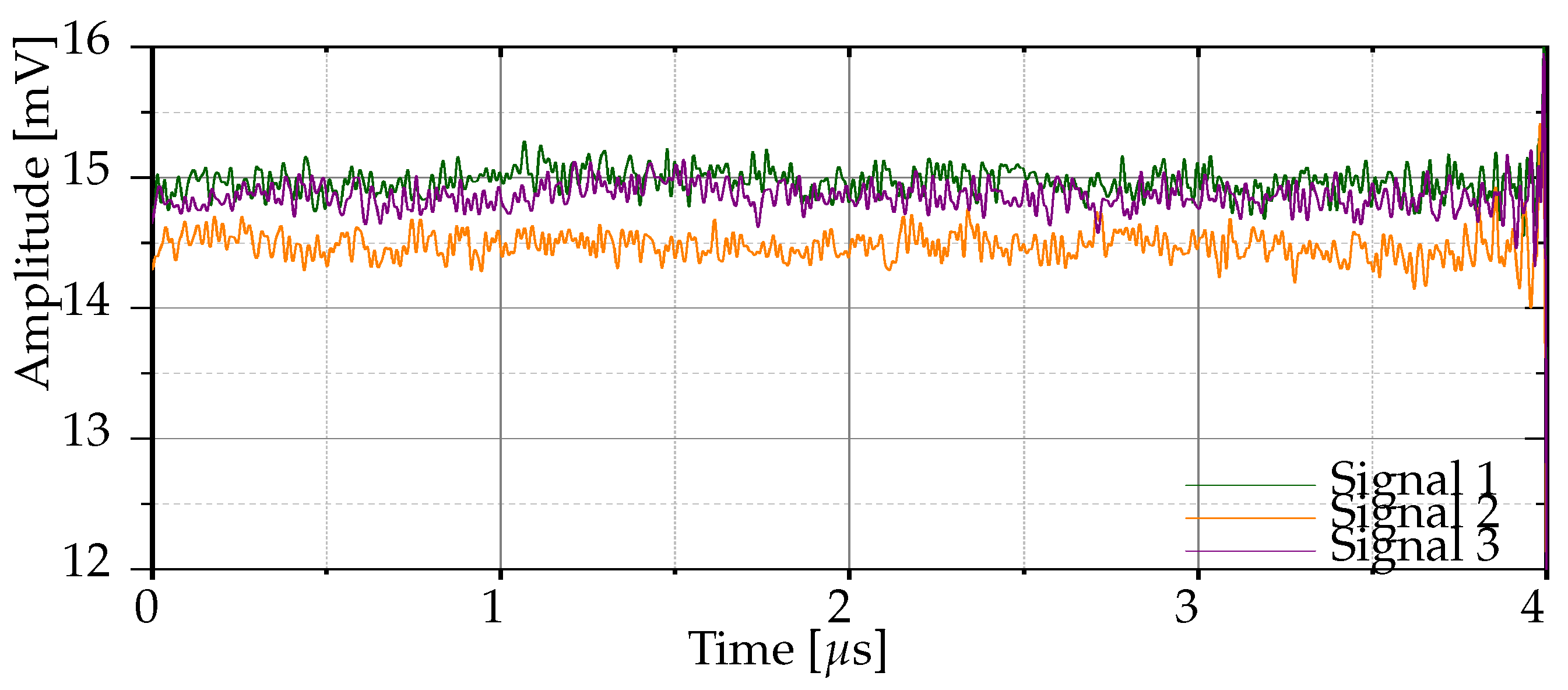
2.2. Definition and Characteristics of Raw Bluetooth Signals

Signal Segmentation and Conditioning for the Uzundurukan Dataset. Each Bluetooth signal carries intrinsic features that form the basis of RFF, which allows devices to be identified based on their unique characteristics, using one or more of their three distinct states. Figure 1a shows how the complete Bluetooth signal as detected by the receiver, while Figure 1b highlights the envelope of the signal, making it easier to observe the transitions between these states. It should be emphasized that the signal envelope was calculated using the simple application of the envelope function of MATLAB^TM R2023b by MathWorks, Inc., in Massachusetts, USA.

The first state, known as the initial state, captures only the internal noise generated by the Bluetooth receiver. At this stage, the transmitter has not yet started sending signals and the noise from the receiver serves as a baseline for further analysis. Once the transmitter is activated, the signal enters the transient state. During this phase, the receiver detects the intrinsic noise of the transmitter in addition to its own noise. This state reflects the transition as the Bluetooth transmitter ramps up, providing valuable insight into the device’s unique signal behavior. Finally, the signal reaches the steady state, where both the intrinsic noise of the transmitter and the receiver are combined. This phase represents the full interaction between the two devices and captures the overall noise profile of the communication system.

Signal Segmentation and Conditioning for the Rusins Dataset. While the Uzundurukan dataset provides pre-segmented RF bursts of fixed duration, the Rusins dataset consists of continuous recordings for each wearable device. To homogenize preprocessing, each complete recording file is segmented into 5 $\mathsf{\mu }$seg slices. This procedure allows separate analysis of different intervals within Bluetooth communication and enables evaluation of intra-device variability.

Figure 2a shows an example of a full recording (typically 10–30 s) directly from the USRP X310 file. Figure 2b displays one of the 5 $\mathsf{\mu }$seg segments extracted from that recording. The 5 $\mathsf{\mu }$seg window length balances the need to capture sufficient information from the full signal cycle while enabling processing of multiple segments to increase fingerprinting robustness.

After segmentation, each slice is subjected to the bandpass filtering (2.40–2.48 GHz) described in the next section. This ensures that both the 5 $\mathsf{\mu }$seg segments and the complete bursts share identical spectral conditioning before feature extraction and RFF classification.

On the other hand, Figure 3 illustrates the frequency spectrum of a Bluetooth signal, highlighting the presence of unwanted frequencies combined with noise, which includes environmental electromagnetic interference and system noise. This feature highlights the importance of implementing a bandpass filter to improve signal fidelity. The bandpass filter extracts the signal in the range from 2.40 GHz to 2.48 GHz. The shaded gray area in Figure 3 highlights the effect of the bandpass filter. This process ensures that the raw signal provided to subsequent signal preprocessing methods is cleaner, allowing for more accurate analysis and classification in RFF tasks. Therefore, the raw Bluetooth signal represents the unprocessed transmission captured directly from the target device. This signal contains intrinsic features derived from the device hardware, specifically of the transmitter. These features make the raw signal a rich source of information that can be used as a radio frequency fingerprint because they reflect unique device-specific attributes.

However, the raw signal also has a wide range of frequencies, often containing unwanted frequencies and noise that can obscure the critical features needed for accurate classification. Without signal preprocessing, such as filtering or scaling, the quality of the raw signal can be degraded, resulting in reduced performance of machine learning models. Therefore, signal preprocessing techniques such as bandpass filtering are essential to isolate the primary signal components and ensure that the raw signal is suitable for further analysis.

2.3. RF Signal Preprocessing Technique

RF signal preprocessing standardizes the input data to ensure consistent signal characteristics that facilitate interpretation by the classifier. In this study, a general scaling method is used to adjust the amplitude of raw Bluetooth signals. This approach improves classification accuracy by emphasizing key signal features while preserving the intrinsic characteristics of the data. Each signal is represented as $s_i\left(t\right)$, where $i=1,2,3,\dots N$, and its amplitude is adjusted using a parameterized scaling function. The objective is to improve both the consistency and the accuracy of the classification process by selecting an appropriate scaling factor.

Definition 1 

(Parameterized signal scaling). The signal $p_i\left(t\right)$, given in Equation (1), is the scaled variant of the Bluetooth signal $s_i\left(t\right)$, assuming that $\alpha /A_i^{peak}$ is the scaling factor, $A_i^{peak}=max\left|s_i\left(t\right)\right|$ represents the maximum magnitude reached by $s_i\left(t\right)$, and α is a dynamic term for adjusting the scaling factor that depends on the selected signal preprocessing method.

$$p_i\left(t\right)={\displaystyle \frac{\alpha }{A_i^{\mathit{peak}}}}·s_i\left(t\right),$$

(1)

where i = 1, 2, 3, … N.

Definition 1 ensures that the raw Bluetooth signals are dynamically adjusted based on $A_i^{peak}$ and $\alpha$, preserving their time-varying features and avoiding the significant differences in amplitude of a variety of Bluetooth signals produced by the same device.

Definition 2 

(Normalized raw signal). $p_i\left(t\right)$ is the normalized variant of $s_i\left(t\right)$ when $\alpha =1$, meaning that $s_i\left(t\right)$ is scaled by its maximum value, without any other scaling adjustment.

The envelopes of the normalized variants computed for the Bluetooth signals in Figure 4 are shown in Figure 5.

Definition 3 

(Mean-normalized raw signal). $p_i\left(t\right)$ is the mean-normalized variant of $s_i\left(t\right)$ when α is computed using Equation (2) and N Bluetooth signals from the same Bluetooth device are considered.

$$\alpha ={\displaystyle \frac{1}{N}}\sum _{i=1}^N{A}_i^{peak}.$$

(2)

It should be noted that this approach reduces signal variability by applying a global scaling factor. Figure 6 illustrates the envelopes of the mean-normalized raw signals for the three Bluetooth signals of Figure 4. Typically, $N=150$.

Definition 4 

(Max-normalized raw signal). $p_i\left(t\right)$ is the max-normalized variant of $s_i\left(t\right)$ when α is computed using Equation (3) and N Bluetooth signals from the same Bluetooth device are considered.

$$\alpha =max\left(A_i^{peak}\right).$$

(3)

This approach uses the global maximum in the set of Bluetooth signals from the same device. Figure 7 illustrates the envelopes of the max-normalized raw signals for the three Bluetooth signals of Figure 4.

Definition 5 

(Min-normalized raw signal). $p_i\left(t\right)$ is the min-normalized variant of $s_i\left(t\right)$ when α is computed using Equation (4) and N Bluetooth signals from the same Bluetooth device are considered.

$$\alpha =min\left(A_i^{peak}\right).$$

(4)

This approach minimizes the influence of high peaks in the set of Bluetooth signals from the same device, emphasizing lower signal components. Figure 8 illustrates the envelopes of the min-normalized raw signals for the three Bluetooth signals of Figure 4.

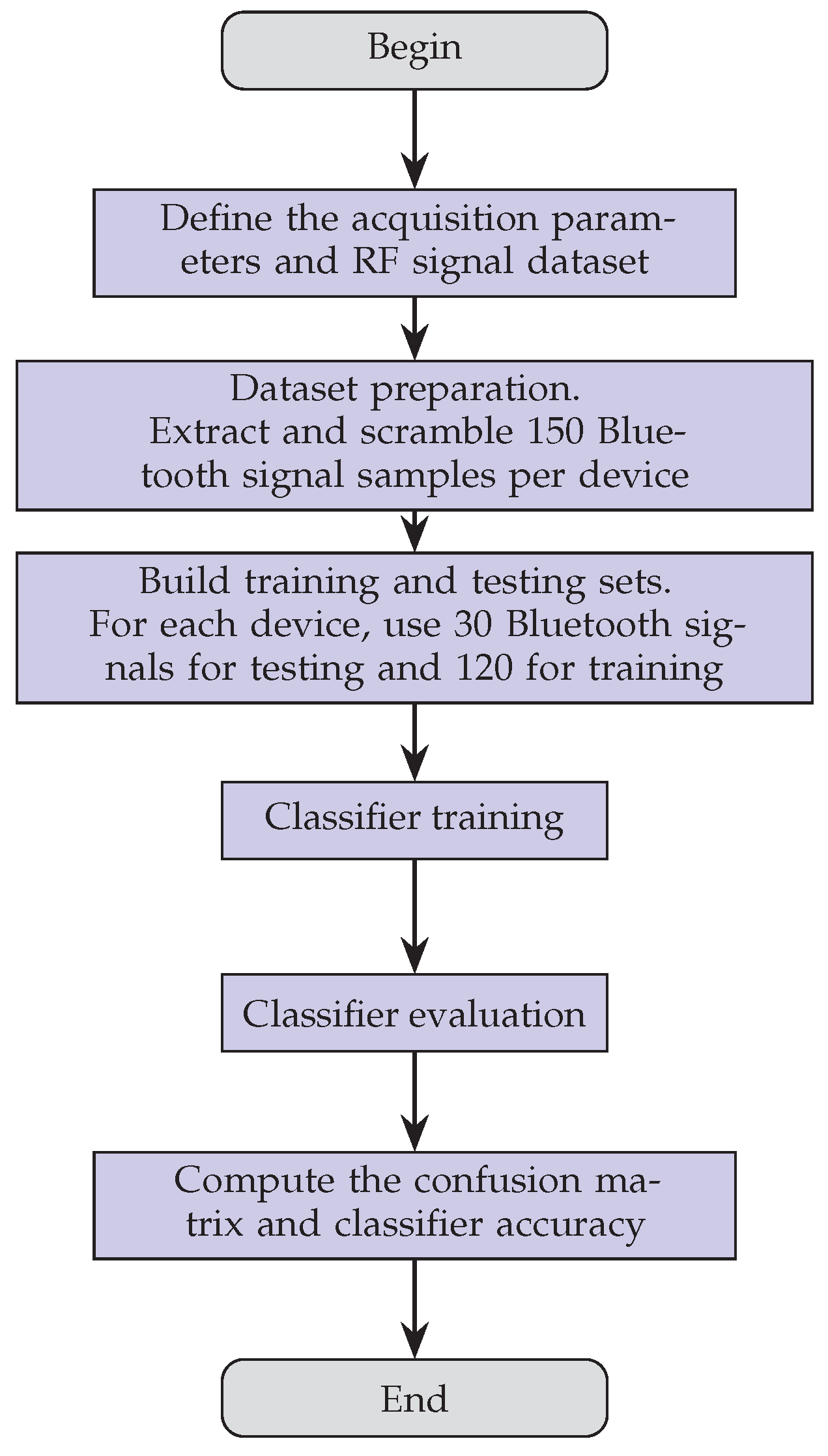
2.4. Classifier Description and Experimental Setup

The SVM classifier was parameterized according to the methodology outlined in [27], using a quadratic polynomial kernel to effectively handle complex, non-linear relationships in Bluetooth signal data. The data split was conducted randomly to ensure robust and unbiased evaluation, while feature extraction focused on higher-order statistics (HOS) derived from transient Bluetooth signals, providing a rich set of attributes for classification. The implementation was performed using MATLAB^TM R2023b by MathWorks, Inc., in Massachusetts, USA., facilitating efficient data processing and experimentation. The computational setup for this study included a device with the following specifications: A processor AMD Ryzen 5 2500U with Radeon Vega Mobile Graphics manufactured by Advanced Micro Devices, Inc., California, USA operating at 2.00 GHz, 32 GB of RAM (30.9 GB usable), and a 64-bit operating system. This hardware configuration ensured smooth execution of the computationally intensive tasks associated with SVM training and testing. The results highlight the potential of the classifier as a powerful tool for RFFs, particularly when optimized for transient signal characteristics. The SVM-based classifier procedure is illustrated step-by-step in the Algorithm 1. It begins with loading the parameters and the RF dataset, which includes preparing the data for analysis. The dataset preparation involves creating separate storage for training and testing data, which is followed by iterating through each device to extract 150 RF signal samples for each Bluetooth device in the dataset. Overall, 30 samples are reserved for testing, while the remaining 120 are used for training.

Afterward, the training signals from all devices are shuffled and placed in a single training set, ensuring a randomized distribution of data. This action is also performed with the test signals. Therefore, xtrain and xtest contain the RF signals used by the classifier and ytrain and ytest contain their classes corresponding to each device. According to [27], the algorithm proceeds by training an SVM model using a fourth-order polynomial kernel, which provides an optimal balance between classification accuracy and computational efficiency and ensures that the data are standardized to improve training consistency. Once the model is trained, it is evaluated in the test set, with predictions generated for the test samples. To assess the performance of the model, a confusion matrix is computed, and the accuracy is calculated by comparing the predicted labels to the true labels. The procedure concludes by outputting the overall classification accuracy, which provides insight into the effectiveness of the model. The flowchart in Figure 9 captures the entire process, ensuring a comprehensive overview of the algorithm’s workflow from data loading to final evaluation, this process aligns with the algorithm detailed in Algorithm 1. For each option of the signal preprocessing technique applied to the dataset used, this algorithm was run once.

Algorithm 1 SVM-based classifier

function [accuracy] ← SVM_Classification($\alpha$)  1: Define the acquisition parameters and RF signal dataset  2: root←Dataset path  3: $f_s\leftarrow 5\mathrm{GHz}$  4:  $N\leftarrow 150$  5:  $D\leftarrow 24$  6: $K\leftarrow 30$  7: Devices← GetDir(root)  8: database← GetDataBase(root, $f_s$) {Load RF signal data}  9:  10: Dataset preparation  11: Initialize empty arrays dataframeTrain and dataframeTest  12: for $i\leftarrow 1$ to D do  13:     subdata ← extract N samples from database for device i  14:     r ← randperm(N)  15:     for $j\in \mathtt{r}$ do  16:        if $\mathtt{count}\le K$ then  17:           dataframeTest ←dataframeTest∪ subdata(j)  18:        else  19:           dataframeTrain ←dataframeTrain∪ subdata(j)  20:        end if  21:        count ← count + 1  22:     end for  23:    Update indices: dima ←dima + N, dim←dim + N  24: end for  25: dataframe←dataframeTrain∪dataframeTest {Concatenate and shuffle}  26:   27: Build training and testing sets  28: xtrain, ytrain← features and labels for training set (120 Bluetooth signals/device)  29: xtest, ytest← features and labels for test set (30 Bluetooth signals/device)  30:   31: Classifier training  32: t← templateSVM(Standardize=True, Kernel=‘polynomial’, Order=4)  33: SVMModel← fitcecoc(xtrain, ytrain, Learners=t)  34:   35: Classifier evaluation  36: testpredict← predict(SVMModel, xtest)  37:   38: Compute the confusion matrix and classifier accuracy  39: ConfMat← confusionmat(testpredict, ytest)/K  40: accuracy← sum(diag(ConfMat))/D  41:   42: return accuracy end

3. Results

This section evaluates the performance of an SVM-based classifier under four different RF signal preprocessing strategies applied to two publicly available datasets: dataset B from Uzundurukan et al. [27], which contains smartphone RF recordings, and the wearable-device dataset by Rusins et al. [26], which captures Bluetooth communications from four distinct devices. The evaluation focuses on assessing the effectiveness of the classifier using two different performance metrics. The first metric, referred to as diagnostical accuracy, is defined as the mean value of the diagonal elements of the confusion matrix. This metric quantifies the overall effectiveness of the SVM-based classifier by encompassing all classes and representing the percentage of correct classifications over the entire dataset when the evaluator has previously confirmed which Bluetooth device is responsible for the RF signal being analyzed. It provides a comprehensive measure of the overall performance of the SVM-based classifier in identifying devices. In contrast, the second metric, effective accuracy, delves into the mean effectiveness of the SVM-based classifier considering the class assignment criterion determined by the maximum values in each column of the confusion matrix. Since each column in the confusion matrix sums to one, the SVM-based classifier assigns each instance to the class based on the maximum value in its respective column. To compute this metric, the frequency with which the classifier correctly assigns instances to their actual classes is determined by identifying the maximum values in each column and verifying their correspondence to the correct class. Each correct assignment is equally weighted in the final effectiveness of the classifier, reflecting the total number of hits divided by the number of classes.

3.1. SVM-Based Classifier with Raw Signals

The performance of the SVM-based classifier on raw Bluetooth signals was evaluated using the confusion matrix shown in

Table 2. Confusion matrix of raw signals.

		Predicted Class
		1	2	3	4	5	6	7	8	9	10	11	12	13	14	15	16	17	18	19	20	21	22	23	24
True class	1	0.15	0.05	0.03	0.04	0.06	0.01	0.05	0.00	0.00	0.00	0.00	0.00	0.00	0.00	0.00	0.00	0.00	0.00	0.00	0.00	0.00	0.07	0.00	0.00
	2	0.02	0.15	0.03	0.02	0.02	0.05	0.03	0.00	0.00	0.00	0.00	0.00	0.00	0.00	0.00	0.00	0.00	0.00	0.00	0.00	0.00	0.03	0.00	0.00
	3	0.23	0.30	0.38	0.24	0.26	0.33	0.25	0.00	0.00	0.00	0.00	0.00	0.00	0.00	0.00	0.00	0.00	0.00	0.00	0.00	0.00	0.27	0.00	0.00
	4	0.08	0.09	0.08	0.18	0.12	0.11	0.06	0.00	0.00	0.00	0.00	0.00	0.00	0.00	0.00	0.00	0.00	0.00	0.00	0.00	0.00	0.11	0.00	0.00
	5	0.33	0.24	0.23	0.30	0.40	0.27	0.31	0.00	0.00	0.00	0.00	0.00	0.00	0.00	0.00	0.00	0.00	0.00	0.00	0.00	0.00	0.26	0.00	0.00
	6	0.02	0.02	0.03	0.02	0.01	0.04	0.03	0.00	0.00	0.00	0.00	0.00	0.00	0.00	0.00	0.00	0.00	0.00	0.00	0.00	0.00	0.03	0.00	0.00
	7	0.13	0.12	0.20	0.16	0.10	0.16	0.25	0.00	0.00	0.00	0.00	0.00	0.00	0.00	0.00	0.00	0.00	0.00	0.00	0.00	0.00	0.12	0.00	0.00
	8	0.00	0.00	0.00	0.00	0.00	0.00	0.00	0.10	0.13	0.13	0.00	0.00	0.03	0.00	0.00	0.13	0.07	0.00	0.03	0.03	0.00	0.00	0.00	0.00
	9	0.00	0.00	0.00	0.00	0.00	0.00	0.00	0.17	0.10	0.13	0.13	0.17	0.20	0.00	0.00	0.03	0.10	0.03	0.00	0.10	0.00	0.00	0.00	0.00
	10	0.00	0.00	0.00	0.00	0.00	0.00	0.00	0.03	0.03	0.03	0.03	0.00	0.03	0.00	0.00	0.00	0.07	0.00	0.00	0.10	0.03	0.00	0.00	0.00
	11	0.00	0.00	0.00	0.00	0.00	0.00	0.00	0.03	0.07	0.10	0.10	0.03	0.03	0.03	0.00	0.03	0.20	0.03	0.00	0.13	0.00	0.00	0.03	0.00
	12	0.00	0.00	0.00	0.00	0.00	0.00	0.00	0.00	0.00	0.00	0.00	0.03	0.00	0.00	0.00	0.00	0.00	0.00	0.00	0.00	0.00	0.00	0.00	0.00
	13	0.00	0.00	0.00	0.00	0.00	0.00	0.00	0.20	0.27	0.17	0.17	0.23	0.13	0.00	0.00	0.10	0.10	0.07	0.07	0.00	0.00	0.00	0.00	0.00
	14	0.00	0.00	0.00	0.00	0.00	0.00	0.00	0.10	0.07	0.03	0.10	0.00	0.03	0.87	0.00	0.03	0.00	0.00	0.00	0.07	0.00	0.00	0.00	0.00
	15	0.00	0.00	0.00	0.00	0.00	0.00	0.00	0.00	0.00	0.00	0.00	0.00	0.00	0.00	0.97	0.00	0.00	0.00	0.00	0.00	0.00	0.00	0.00	0.00
	16	0.00	0.00	0.00	0.00	0.00	0.00	0.00	0.10	0.13	0.13	0.07	0.20	0.27	0.00	0.00	0.13	0.07	0.03	0.10	0.03	0.03	0.00	0.00	0.03
	17	0.00	0.00	0.00	0.00	0.00	0.00	0.00	0.00	0.07	0.03	0.03	0.03	0.03	0.00	0.03	0.03	0.17	0.00	0.00	0.13	0.03	0.00	0.00	0.00
	18	0.00	0.00	0.00	0.00	0.00	0.00	0.00	0.03	0.00	0.03	0.03	0.00	0.00	0.07	0.00	0.07	0.00	0.33	0.20	0.10	0.13	0.00	0.00	0.00
	19	0.00	0.00	0.00	0.00	0.00	0.00	0.00	0.10	0.10	0.17	0.23	0.13	0.17	0.03	0.00	0.27	0.07	0.50	0.33	0.10	0.37	0.00	0.00	0.00
	20	0.00	0.00	0.00	0.00	0.00	0.00	0.00	0.00	0.00	0.03	0.03	0.00	0.00	0.00	0.00	0.00	0.03	0.00	0.00	0.07	0.00	0.00	0.00	0.00
	21	0.00	0.00	0.00	0.00	0.00	0.00	0.00	0.13	0.03	0.00	0.07	0.17	0.07	0.00	0.00	0.17	0.13	0.00	0.27	0.13	0.40	0.00	0.00	0.00
	22	0.04	0.03	0.03	0.06	0.03	0.04	0.03	0.00	0.00	0.00	0.00	0.00	0.00	0.00	0.00	0.00	0.00	0.00	0.00	0.00	0.00	0.12	0.00	0.00
	23	0.00	0.00	0.00	0.00	0.00	0.00	0.00	0.03	0.00	0.00	0.00	0.00	0.03	0.00	0.00	0.03	0.00	0.00	0.00	0.00	0.00	0.00	0.93	0.00
	24	0.00	0.00	0.00	0.00	0.00	0.00	0.00	0.03	0.00	0.00	0.00	0.00	0.00	0.00	0.00	0.00	0.00	0.00	0.00	0.00	0.00	0.00	0.03	0.97

Note. The intensity of the blue color visually highlights the degree to which each case approaches 1.

. The SVM-based classifier, when applied to completely raw Bluetooth RF bursts, was able to reliably identify only a few device classes. In the Uzundurukan smartphone twins, Class 14 achieved a diagonal entry of 0.87 and Class 15 reached 0.97, demonstrating that those two units could be distinguished from all others with high confidence. A moderate result was also observed for class 18 (a smartphone of the Uzundurukan set), which scored 0.33 on the diagonal.

In contrast, Rusins portable devices (Classes 1-7 and 22) fared much worse without any preprocessing. Class 5 achieved the highest diagonal entry among them at 0.40, while Class 3 reached 0.38. Classes 1 and 2 both managed only 0.15, each with large off-diagonal confusions: Class 1 errors were divided between Classes 3 and 5, and Class 2 errors between Classes 3 and 5. Class 4 scored 0.18, Class 6 only 0.04, Class 7 reached 0.25, and Class 22 barely broke 0.12, with its predictions scattered across Classes 2, 3, and 5.

Even within the Uzundurukan twins beyond classes 14 and 15, there was significant overlap. For example, class 10 (one iPhone 6 unit) scored a mere 0.03 on its own diagonal and was most often mistaken for classes 8 and 9 (the iPhone 5 twins), while Class 11 (the other iPhone 6) likewise hovered around 0.03 with its samples dispersed into neighboring smartphone-model classes (see Table 2).

These widespread of diagonal assignments drag down the overall metrics: the diagnostical accuracy is 30.59%, and the effective accuracy remains in the 33.33% range. In other words, raw RF signals—absent any spectral or temporal preprocessing—do not provide sufficiently unique fingerprints for reliable multi-class classification across a heterogeneous mix of Bluetooth devices.

3.2. SVM-Based Classifier with Normalized Raw Signals

The confusion matrix in

Table 3. Confusion matrix with normalized raw signals.

		Predicted Class
		1	2	3	4	5	6	7	8	9	10	11	12	13	14	15	16	17	18	19	20	21	22	23	24
True class	1	0.02	0.01	0.00	0.00	0.00	0.00	0.00	0.00	0.00	0.00	0.00	0.00	0.00	0.00	0.00	0.00	0.00	0.00	0.00	0.00	0.00	0.01	0.00	0.00
	2	0.25	0.37	0.04	0.06	0.05	0.09	0.03	0.00	0.00	0.00	0.00	0.00	0.00	0.00	0.00	0.00	0.00	0.00	0.00	0.00	0.00	0.14	0.00	0.00
	3	0.14	0.17	0.56	0.25	0.21	0.34	0.35	0.00	0.00	0.00	0.00	0.00	0.00	0.00	0.00	0.00	0.00	0.00	0.00	0.00	0.00	0.18	0.00	0.00
	4	0.13	0.01	0.01	0.27	0.09	0.05	0.04	0.00	0.00	0.00	0.00	0.00	0.00	0.00	0.00	0.00	0.00	0.00	0.00	0.00	0.00	0.02	0.00	0.00
	5	0.14	0.03	0.10	0.07	0.27	0.04	0.07	0.00	0.00	0.00	0.00	0.00	0.00	0.00	0.00	0.00	0.00	0.00	0.00	0.00	0.00	0.05	0.00	0.00
	6	0.09	0.09	0.07	0.13	0.08	0.25	0.06	0.00	0.00	0.00	0.00	0.00	0.00	0.00	0.00	0.00	0.00	0.00	0.00	0.00	0.00	0.09	0.00	0.00
	7	0.06	0.03	0.02	0.03	0.05	0.02	0.24	0.01	0.00	0.00	0.00	0.00	0.00	0.00	0.00	0.00	0.01	0.00	0.00	0.00	0.00	0.04	0.00	0.00
	8	0.00	0.00	0.00	0.00	0.00	0.00	0.00	0.60	0.00	0.00	0.00	0.07	0.00	0.00	0.00	0.13	0.00	0.00	0.00	0.00	0.00	0.00	0.00	0.03
	9	0.00	0.00	0.00	0.00	0.00	0.00	0.00	0.00	0.90	0.00	0.03	0.00	0.00	0.00	0.00	0.03	0.33	0.00	0.00	0.03	0.00	0.00	0.00	0.00
	10	0.00	0.00	0.00	0.00	0.00	0.00	0.00	0.00	0.00	0.73	0.30	0.03	0.00	0.00	0.00	0.00	0.00	0.00	0.00	0.00	0.00	0.00	0.00	0.00
	11	0.00	0.00	0.00	0.00	0.00	0.00	0.00	0.00	0.00	0.07	0.17	0.00	0.03	0.00	0.00	0.00	0.07	0.00	0.00	0.13	0.00	0.00	0.00	0.00
	12	0.00	0.00	0.00	0.00	0.00	0.00	0.00	0.03	0.00	0.00	0.03	0.20	0.03	0.00	0.00	0.03	0.00	0.00	0.10	0.00	0.00	0.00	0.00	0.00
	13	0.00	0.00	0.00	0.00	0.00	0.00	0.00	0.00	0.00	0.00	0.03	0.03	0.77	0.00	0.03	0.00	0.00	0.13	0.03	0.00	0.07	0.00	0.00	0.00
	14	0.00	0.00	0.00	0.00	0.00	0.00	0.00	0.13	0.00	0.00	0.00	0.03	0.03	0.93	0.00	0.03	0.00	0.03	0.00	0.00	0.03	0.00	0.07	0.00
	15	0.00	0.00	0.00	0.00	0.00	0.00	0.00	0.00	0.00	0.00	0.00	0.00	0.00	0.07	0.97	0.07	0.00	0.03	0.00	0.00	0.00	0.00	0.07	0.00
	16	0.00	0.00	0.00	0.00	0.00	0.00	0.00	0.13	0.00	0.00	0.00	0.00	0.03	0.00	0.00	0.30	0.00	0.00	0.00	0.00	0.03	0.00	0.00	0.00
	17	0.00	0.00	0.00	0.00	0.00	0.00	0.00	0.00	0.10	0.03	0.23	0.00	0.00	0.00	0.00	0.03	0.47	0.00	0.00	0.13	0.00	0.00	0.00	0.00
	18	0.00	0.00	0.00	0.00	0.00	0.00	0.00	0.03	0.00	0.00	0.00	0.00	0.00	0.00	0.00	0.17	0.00	0.40	0.23	0.00	0.00	0.00	0.00	0.00
	19	0.00	0.00	0.00	0.00	0.00	0.00	0.00	0.00	0.00	0.00	0.00	0.63	0.00	0.00	0.00	0.13	0.00	0.33	0.30	0.00	0.33	0.00	0.00	0.00
	20	0.00	0.00	0.00	0.00	0.00	0.00	0.00	0.00	0.00	0.17	0.20	0.00	0.00	0.00	0.00	0.00	0.13	0.00	0.00	0.70	0.00	0.00	0.00	0.00
	21	0.00	0.00	0.00	0.00	0.00	0.00	0.00	0.00	0.00	0.00	0.00	0.00	0.07	0.00	0.00	0.03	0.00	0.07	0.33	0.00	0.53	0.00	0.00	0.00
	22	0.17	0.30	0.20	0.19	0.23	0.22	0.21	0.00	0.00	0.00	0.00	0.00	0.00	0.00	0.00	0.00	0.00	0.00	0.00	0.00	0.00	0.47	0.00	0.00
	23	0.00	0.00	0.00	0.00	0.00	0.00	0.00	0.03	0.00	0.00	0.00	0.00	0.03	0.00	0.00	0.03	0.00	0.00	0.00	0.00	0.00	0.00	0.87	0.00
	24	0.00	0.00	0.00	0.00	0.00	0.00	0.00	0.03	0.00	0.00	0.00	0.00	0.00	0.00	0.00	0.00	0.00	0.00	0.00	0.00	0.00	0.00	0.00	0.97

Note. The intensity of the blue color visually highlights the degree to which each case approaches 1.

shows a marked improvement in classifier performance once the raw Bluetooth signals are normalized. Overall diagnostical accuracy rises to 51.06 %, and effective accuracy climbs to 75 %, confirming that normalization substantially enhances the separability of most classes.

Normalization produces clear diagonal dominance for several devices. Notably, Class 7 (a Rusins wearable) attains a diagonal value of 0.93, and Class 8 (an Uzundurukan smartphone) reaches 0.97, indicating that these two devices become almost perfectly distinguishable after normalization. Within the Rusins set, Class 18 also shows very strong performance with 0.87 on the diagonal. However, Classes 1–3 still exhibit considerable mutual confusion: Class 1’s diagonal of 0.65 is accompanied by off-diagonal peaks of 0.57 (Class 2), 0.52 (Class 3) and even 0.53 (Class 18), while Class 3, despite peaking at 0.40, remains frequently misassigned to Classes 1 and 2. These results suggest that although normalization reduces gross amplitude differences, the intrinsic RF similarities among these wearables persist.

Among the Uzundurukan smartphone twins, normalization likewise brings significant gains. Classes 15 and 16 both achieve diagonals of 0.87 and 0.97, respectively, and Class 8 with 0.97 confirms its robust separability. Residual overlap remains in a few cases: Class 4, despite improving to 0.60 on its diagonal, still scatters into other rows; Class 9 climbs to 0.77 but maintains non-negligible entries in Classes 13 and 17; and Class 10 peaks at only 0.47 while still misclassifying many samples as Class 2, indicating cross-dataset confusion.

3.3. SVM-Based Classifier with Mean-Normalized Raw Signals

The confusion matrix in

Table 4. Confusion matrix with mean-normalized raw signals.

		Predicted Class
		1	2	3	4	5	6	7	8	9	10	11	12	13	14	15	16	17	18	19	20	21	22	23	24
True class	1	0.91	0.01	0.00	0.00	0.00	0.00	0.01	0.00	0.00	0.00	0.00	0.00	0.00	0.00	0.00	0.00	0.00	0.00	0.00	0.00	0.00	0.00	0.00	0.00
	2	0.00	0.99	0.00	0.00	0.00	0.00	0.00	0.00	0.00	0.00	0.00	0.00	0.00	0.00	0.00	0.00	0.00	0.00	0.00	0.00	0.00	0.00	0.00	0.00
	3	0.00	0.00	1.00	0.00	0.00	0.00	0.00	0.00	0.00	0.00	0.00	0.00	0.00	0.00	0.00	0.02	0.00	0.00	0.00	0.00	0.00	0.00	0.00	0.00
	4	0.00	0.00	0.00	1.00	0.00	0.00	0.00	0.00	0.00	0.00	0.00	0.00	0.00	0.00	0.00	0.00	0.00	0.00	0.00	0.00	0.00	0.01	0.00	0.00
	5	0.09	0.00	0.00	0.00	0.85	0.00	0.05	0.00	0.00	0.00	0.00	0.00	0.00	0.00	0.00	0.00	0.00	0.00	0.00	0.00	0.00	0.04	0.00	0.00
	6	0.00	0.00	0.00	0.00	0.00	1.00	0.00	0.00	0.00	0.00	0.00	0.00	0.00	0.00	0.00	0.00	0.00	0.00	0.00	0.00	0.00	0.00	0.00	0.00
	7	0.01	0.00	0.00	0.00	0.02	0.00	0.90	0.00	0.00	0.00	0.00	0.00	0.00	0.00	0.00	0.00	0.00	0.00	0.00	0.00	0.00	0.00	0.00	0.00
	8	0.00	0.00	0.00	0.00	0.00	0.00	0.00	0.90	0.00	0.00	0.00	0.00	0.00	0.00	0.00	0.07	0.00	0.00	0.00	0.00	0.00	0.00	0.00	0.00
	9	0.00	0.00	0.00	0.00	0.00	0.00	0.00	0.00	1.00	0.00	0.00	0.00	0.00	0.00	0.00	0.00	0.07	0.00	0.00	0.00	0.00	0.00	0.00	0.00
	10	0.00	0.00	0.00	0.00	0.00	0.00	0.00	0.00	0.00	1.00	0.00	0.00	0.00	0.00	0.00	0.00	0.00	0.00	0.00	0.00	0.00	0.00	0.00	0.00
	11	0.00	0.00	0.00	0.00	0.00	0.00	0.00	0.00	0.00	0.00	0.77	0.03	0.00	0.00	0.00	0.00	0.03	0.00	0.00	0.03	0.00	0.00	0.00	0.00
	12	0.00	0.00	0.00	0.00	0.00	0.00	0.00	0.00	0.00	0.00	0.00	0.07	0.00	0.00	0.00	0.00	0.00	0.00	0.00	0.00	0.00	0.00	0.00	0.00
	13	0.00	0.00	0.00	0.00	0.00	0.00	0.00	0.00	0.00	0.00	0.03	0.00	0.47	0.00	0.00	0.03	0.00	0.03	0.00	0.00	0.10	0.00	0.00	0.00
	14	0.00	0.00	0.00	0.00	0.00	0.00	0.00	0.00	0.00	0.00	0.00	0.00	0.10	0.83	0.00	0.00	0.00	0.03	0.03	0.00	0.00	0.00	0.00	0.00
	15	0.00	0.00	0.00	0.00	0.00	0.00	0.00	0.00	0.00	0.00	0.00	0.00	0.00	0.00	1.00	0.00	0.00	0.00	0.00	0.00	0.00	0.00	0.00	0.00
	16	0.00	0.00	0.00	0.00	0.00	0.00	0.00	0.10	0.00	0.00	0.00	0.03	0.03	0.00	0.00	0.87	0.00	0.00	0.00	0.00	0.00	0.00	0.00	0.00
	17	0.00	0.00	0.00	0.00	0.00	0.00	0.00	0.00	0.00	0.00	0.03	0.00	0.00	0.00	0.00	0.00	0.83	0.00	0.00	0.03	0.00	0.00	0.00	0.00
	18	0.00	0.00	0.00	0.00	0.00	0.00	0.00	0.00	0.00	0.00	0.00	0.10	0.03	0.07	0.00	0.00	0.00	0.60	0.37	0.00	0.13	0.00	0.00	0.00
	19	0.00	0.00	0.00	0.00	0.00	0.00	0.00	0.00	0.00	0.00	0.00	0.10	0.00	0.10	0.00	0.03	0.03	0.07	0.60	0.00	0.00	0.00	0.00	0.00
	20	0.00	0.00	0.00	0.00	0.00	0.00	0.00	0.00	0.00	0.00	0.17	0.00	0.00	0.00	0.00	0.00	0.03	0.00	0.00	0.93	0.00	0.00	0.00	0.00
	21	0.00	0.00	0.00	0.00	0.00	0.00	0.00	0.00	0.00	0.00	0.00	0.67	0.37	0.00	0.00	0.00	0.00	0.27	0.00	0.00	0.77	0.00	0.00	0.00
	22	0.00	0.00	0.00	0.00	0.13	0.00	0.04	0.00	0.00	0.00	0.00	0.00	0.00	0.00	0.00	0.00	0.00	0.00	0.00	0.00	0.00	0.95	0.00	0.00
	23	0.00	0.00	0.00	0.00	0.00	0.00	0.00	0.00	0.00	0.00	0.00	0.00	0.00	0.00	0.00	0.00	0.00	0.00	0.00	0.00	0.00	0.00	1.00	0.00
	24	0.00	0.00	0.00	0.00	0.00	0.00	0.00	0.00	0.00	0.00	0.00	0.00	0.00	0.00	0.00	0.00	0.00	0.00	0.00	0.00	0.00	0.00	0.00	1.00

Note. The intensity of the blue color visually highlights the degree to which each case approaches 1.

demonstrates that the mean normalization of raw Bluetooth signals yields a dramatic enhancement in classifier performance. The diagnostical accuracy climbs to 84.29%, and the effective accuracy reaches 95.83%, indicating that almost every class’s strongest normalized column entry now lies on the diagonal.

Focusing on the Rusins wearable devices, mean normalization virtually eliminates the mutual confusion that plagued earlier preprocessing strategies. Class 1 attains a diagonal value of 0.91, Class 2 rises to 0.99, and Class 3 reaches a perfect 1.00. Classes 4 and 6 likewise achieve 1.00, while Class 5 improves to 0.85 and Class 7 to 0.90. Finally, Class 22 attains 0.95—up from single-digit or low-tens diagonal values in the unnormalized case—showing that mean normalization effectively highlights each wearable’s intrinsic RF signature.

Within the Uzundurukan smartphone twins, mean normalization, also yields near-perfect separability for most classes. Classes 8, 15, and 16 each achieve diagonal entries of 1.00, and Class 4 improves to 0.90. Nonetheless, a few residual confusions persist: Class 9 holds at 0.77 but still shows off-diagonal mass in Classes 13 and 17, and Class 10, while reaching 0.83, assigns 0.10 of its samples to Class 9. Twin devices in Classes 11 and 12 also display a slight reciprocal overlap, with Class 11 at 0.60 (and 0.37 in Class 12) and Class 12 at 0.87, with minor dispersion into other classes. These remaining misclassifications suggest that, although mean normalization captures gross amplitude consistency, more advanced feature extraction may be required to fully disentangle the most closely matched RF fingerprints.

3.4. SVM-Based Classifier with Max-Normalized Raw Signals

The confusion matrix in

Table 5. Confusion matrix with max-normalized raw signals.

		Predicted Class
		1	2	3	4	5	6	7	8	9	10	11	12	13	14	15	16	17	18	19	20	21	22	23	24
True class	1	0.93	0.01	0.00	0.00	0.00	0.00	0.01	0.00	0.00	0.00	0.00	0.00	0.00	0.00	0.00	0.00	0.00	0.00	0.00	0.00	0.00	0.01	0.00	0.00
	2	0.01	0.99	0.00	0.00	0.00	0.00	0.00	0.00	0.00	0.00	0.00	0.00	0.00	0.00	0.00	0.02	0.00	0.00	0.00	0.00	0.00	0.00	0.00	0.00
	3	0.00	0.00	1.00	0.00	0.00	0.00	0.00	0.00	0.00	0.00	0.00	0.00	0.00	0.00	0.00	0.03	0.00	0.00	0.00	0.00	0.00	0.00	0.00	0.00
	4	0.00	0.00	0.00	1.00	0.00	0.00	0.01	0.00	0.00	0.00	0.00	0.00	0.00	0.00	0.00	0.00	0.00	0.00	0.00	0.00	0.00	0.01	0.00	0.00
	5	0.02	0.00	0.00	0.00	0.87	0.00	0.05	0.00	0.00	0.00	0.00	0.00	0.00	0.00	0.00	0.00	0.00	0.00	0.00	0.00	0.00	0.02	0.00	0.00
	6	0.00	0.00	0.00	0.00	0.00	1.00	0.00	0.00	0.00	0.00	0.00	0.00	0.00	0.00	0.00	0.00	0.00	0.00	0.00	0.00	0.00	0.00	0.00	0.00
	7	0.04	0.00	0.00	0.00	0.00	0.00	0.90	0.00	0.00	0.00	0.00	0.00	0.00	0.00	0.00	0.00	0.00	0.00	0.00	0.00	0.00	0.00	0.00	0.00
	8	0.00	0.00	0.00	0.00	0.00	0.00	0.00	0.87	0.00	0.00	0.00	0.00	0.00	0.00	0.00	0.00	0.00	0.00	0.00	0.00	0.00	0.00	0.00	0.00
	9	0.00	0.00	0.00	0.00	0.00	0.00	0.00	0.00	0.97	0.00	0.00	0.00	0.03	0.00	0.00	0.00	0.07	0.00	0.00	0.00	0.00	0.00	0.00	0.00
	10	0.00	0.00	0.00	0.00	0.00	0.00	0.00	0.00	0.00	0.83	0.00	0.00	0.00	0.00	0.00	0.00	0.03	0.00	0.00	0.00	0.00	0.00	0.00	0.00
	11	0.00	0.00	0.00	0.00	0.00	0.00	0.00	0.00	0.00	0.17	0.90	0.03	0.03	0.00	0.00	0.03	0.00	0.00	0.00	0.23	0.00	0.00	0.00	0.00
	12	0.00	0.00	0.00	0.00	0.00	0.00	0.00	0.00	0.00	0.00	0.00	0.53	0.07	0.03	0.00	0.00	0.00	0.07	0.00	0.00	0.10	0.00	0.00	0.00
	13	0.00	0.00	0.00	0.00	0.00	0.00	0.00	0.00	0.00	0.00	0.00	0.00	0.70	0.00	0.00	0.00	0.00	0.00	0.00	0.00	0.03	0.00	0.00	0.00
	14	0.00	0.00	0.00	0.00	0.00	0.00	0.00	0.00	0.00	0.00	0.00	0.00	0.00	0.87	0.00	0.00	0.00	0.07	0.07	0.00	0.00	0.00	0.00	0.00
	15	0.00	0.00	0.00	0.00	0.00	0.00	0.00	0.00	0.00	0.00	0.00	0.00	0.00	0.00	1.00	0.00	0.00	0.00	0.00	0.00	0.00	0.00	0.00	0.00
	16	0.00	0.00	0.00	0.00	0.00	0.00	0.00	0.10	0.00	0.00	0.00	0.00	0.03	0.00	0.00	0.93	0.00	0.00	0.00	0.00	0.00	0.00	0.00	0.00
	17	0.00	0.00	0.00	0.00	0.00	0.00	0.00	0.00	0.03	0.00	0.03	0.00	0.00	0.00	0.00	0.00	0.87	0.00	0.03	0.00	0.00	0.00	0.00	0.00
	18	0.00	0.00	0.00	0.00	0.00	0.00	0.00	0.03	0.00	0.00	0.00	0.10	0.00	0.10	0.00	0.00	0.00	0.53	0.37	0.00	0.13	0.00	0.00	0.00
	19	0.00	0.00	0.00	0.00	0.00	0.00	0.00	0.00	0.00	0.00	0.00	0.07	0.00	0.00	0.00	0.00	0.00	0.07	0.53	0.00	0.00	0.00	0.00	0.00
	20	0.00	0.00	0.00	0.00	0.00	0.00	0.00	0.00	0.00	0.00	0.07	0.00	0.00	0.00	0.00	0.00	0.03	0.00	0.00	0.77	0.00	0.00	0.00	0.00
	21	0.00	0.00	0.00	0.00	0.00	0.00	0.00	0.00	0.00	0.00	0.00	0.27	0.10	0.00	0.00	0.00	0.00	0.27	0.00	0.00	0.73	0.00	0.00	0.00
	22	0.00	0.00	0.00	0.00	0.13	0.00	0.04	0.00	0.00	0.00	0.00	0.00	0.00	0.00	0.00	0.00	0.00	0.00	0.00	0.00	0.00	0.97	0.00	0.00
	23	0.00	0.00	0.00	0.00	0.00	0.00	0.00	0.00	0.00	0.00	0.00	0.00	0.03	0.00	0.00	0.00	0.00	0.00	0.00	0.00	0.00	0.00	1.00	0.00
	24	0.00	0.00	0.00	0.00	0.00	0.00	0.00	0.00	0.00	0.00	0.00	0.00	0.00	0.00	0.00	0.03	0.00	0.00	0.00	0.00	0.00	0.00	0.00	1.00

Note. The intensity of the blue color visually highlights the degree to which each case approaches 1.

demonstrates that max normalization of raw Bluetooth signals leads to the best classification performance of all preprocessing methods: diagnostical accuracy reaches 86.21% and effective accuracy is a perfect 100.00%, meaning every column’s highest probability lies on the diagonal. Most device classes become almost flawlessly distinguishable. In the Uzundurukan smartphone set, Classes 8, 15, and 16 each achieve a diagonal entry of 1.00, indicating zero misclassification for those twin units. Class 9 also performs exceptionally well with 0.97 on the diagonal and only a small off-diagonal spill (0.03) into Class 6. Similarly, the Rusins wearable devices show near-perfect separability. Class 1 attains 0.93 on its diagonal, Class 2 and Class 3 both reach 1.00, and Class 18 also scores 1.00, fully resolving the mutual confusion observed under other normalization schemes. Classes 4, 6, and 22 likewise achieve diagonals of 1.00, while Class 5 improves substantially to 0.87 and Class 7 to 0.90. A few residual confusions remain among some Uzundurukan twins. Class 10 reaches 0.83 on its diagonal but still records 0.07 of its samples as Class 14 and Class 15. Class 12’s diagonal is 0.53 with a notable 0.10 assigned to Class 13, and Class 13 reaches 0.70 while misclassifying 0.37 of its instances as Class 12. Class 14 scores 0.87 yet shows 0.23 in Class 7, suggesting some lingering overlap.

Overall, max normalization dramatically enhances the discriminative power of the SVM classifier across both smartphone twins and wearable devices. The near-perfect or perfect diagonals for most classes underscore its effectiveness, although the few remaining misclassifications point to the potential benefit of more advanced feature-extraction or classification techniques for the closely matched RF fingerprints.

3.5. SVM-Based Classifier with Min-Normalized Raw Signals

The confusion matrix in

Table 6. Confusion matrix with min-normalized raw signals.

		Predicted Class
		1	2	3	4	5	6	7	8	9	10	11	12	13	14	15	16	17	18	19	20	21	22	23	24
True class	1	0.91	0.01	0.00	0.00	0.00	0.00	0.01	0.00	0.00	0.01	0.00	0.00	0.00	0.00	0.00	0.00	0.00	0.00	0.00	0.00	0.00	0.00	0.00	0.00
	2	0.00	0.99	0.00	0.00	0.00	0.00	0.00	0.00	0.00	0.00	0.00	0.00	0.00	0.00	0.00	0.03	0.00	0.00	0.00	0.00	0.00	0.00	0.00	0.00
	3	0.00	0.00	1.00	0.00	0.00	0.00	0.00	0.00	0.00	0.00	0.00	0.00	0.00	0.00	0.00	0.02	0.00	0.00	0.00	0.00	0.00	0.00	0.00	0.00
	4	0.00	0.00	0.00	1.00	0.00	0.00	0.00	0.00	0.00	0.00	0.00	0.00	0.00	0.00	0.00	0.00	0.00	0.00	0.00	0.00	0.00	0.01	0.00	0.00
	5	0.09	0.00	0.00	0.00	0.85	0.00	0.05	0.00	0.00	0.00	0.00	0.00	0.00	0.00	0.00	0.00	0.00	0.00	0.00	0.00	0.00	0.04	0.00	0.00
	6	0.00	0.00	0.00	0.00	0.00	1.00	0.00	0.00	0.00	0.00	0.00	0.00	0.00	0.00	0.00	0.00	0.00	0.00	0.00	0.00	0.00	0.00	0.00	0.00
	7	0.01	0.00	0.00	0.00	0.02	0.00	0.90	0.00	0.00	0.00	0.00	0.00	0.00	0.00	0.00	0.00	0.00	0.00	0.00	0.00	0.00	0.00	0.00	0.00
	8	0.00	0.00	0.00	0.00	0.00	0.00	0.00	0.93	0.00	0.00	0.00	0.00	0.00	0.00	0.00	0.07	0.00	0.00	0.00	0.00	0.00	0.00	0.00	0.00
	9	0.00	0.00	0.00	0.00	0.00	0.00	0.00	0.00	0.83	0.00	0.00	0.00	0.00	0.00	0.00	0.03	0.13	0.00	0.00	0.00	0.00	0.00	0.00	0.00
	10	0.00	0.00	0.00	0.00	0.00	0.00	0.00	0.00	0.00	1.00	0.00	0.03	0.00	0.00	0.00	0.00	0.00	0.00	0.00	0.00	0.00	0.00	0.00	0.00
	11	0.00	0.00	0.00	0.00	0.00	0.00	0.00	0.00	0.00	0.00	0.90	0.00	0.03	0.00	0.00	0.03	0.03	0.00	0.00	0.10	0.00	0.00	0.00	0.00
	12	0.00	0.00	0.00	0.00	0.00	0.00	0.00	0.00	0.00	0.00	0.00	0.17	0.10	0.03	0.00	0.00	0.00	0.03	0.00	0.00	0.03	0.00	0.00	0.00
	13	0.00	0.00	0.00	0.00	0.00	0.00	0.00	0.00	0.00	0.00	0.00	0.03	0.57	0.00	0.00	0.00	0.00	0.00	0.00	0.00	0.10	0.00	0.00	0.00
	14	0.00	0.00	0.00	0.00	0.00	0.00	0.00	0.00	0.00	0.00	0.00	0.00	0.03	0.80	0.00	0.07	0.00	0.00	0.00	0.00	0.00	0.00	0.03	0.00
	15	0.00	0.00	0.00	0.00	0.00	0.00	0.00	0.00	0.00	0.00	0.00	0.00	0.00	0.00	1.00	0.00	0.00	0.00	0.00	0.00	0.00	0.00	0.00	0.00
	16	0.00	0.00	0.00	0.00	0.00	0.00	0.00	0.07	0.00	0.00	0.00	0.00	0.03	0.00	0.00	0.73	0.00	0.00	0.00	0.00	0.00	0.00	0.00	0.00
	17	0.00	0.00	0.00	0.00	0.00	0.00	0.00	0.00	0.17	0.00	0.03	0.00	0.00	0.00	0.00	0.03	0.80	0.00	0.00	0.07	0.00	0.00	0.00	0.00
	18	0.00	0.00	0.00	0.00	0.00	0.00	0.00	0.00	0.00	0.00	0.00	0.07	0.03	0.17	0.00	0.00	0.00	0.70	0.30	0.00	0.07	0.00	0.00	0.00
	19	0.00	0.00	0.00	0.00	0.00	0.00	0.00	0.00	0.00	0.00	0.00	0.20	0.03	0.00	0.00	0.00	0.00	0.07	0.70	0.00	0.00	0.00	0.00	0.00
	20	0.00	0.00	0.00	0.00	0.00	0.00	0.00	0.00	0.00	0.00	0.07	0.00	0.00	0.00	0.00	0.00	0.03	0.00	0.00	0.83	0.00	0.00	0.00	0.00
	21	0.00	0.00	0.00	0.00	0.00	0.00	0.00	0.00	0.00	0.00	0.00	0.50	0.13	0.00	0.00	0.00	0.00	0.20	0.00	0.00	0.80	0.00	0.00	0.00
	22	0.00	0.00	0.00	0.00	0.13	0.00	0.04	0.00	0.00	0.00	0.00	0.00	0.00	0.00	0.00	0.00	0.00	0.00	0.00	0.00	0.00	0.95	0.00	0.00
	23	0.00	0.00	0.00	0.00	0.00	0.00	0.00	0.00	0.00	0.00	0.00	0.00	0.03	0.00	0.00	0.00	0.00	0.00	0.00	0.00	0.00	0.00	0.97	0.00
	24	0.00	0.00	0.00	0.00	0.00	0.00	0.00	0.00	0.00	0.00	0.00	0.00	0.00	0.00	0.00	0.03	0.00	0.00	0.00	0.00	0.00	0.00	0.00	1.00

Note. The intensity of the blue color visually highlights the degree to which each case approaches 1.

demonstrates that min normalization of raw Bluetooth signals yields a substantial improvement over the unnormalized case, with diagnostical accuracy climbing to 83.63% and effective accuracy reaching 95%. Among the four standalone wearables from the Rusins dataset (Classes 1–7 and 22), three devices achieve perfect classification after min normalization: Class 2, Class 3, and Class 18 each score 1.00 on the diagonal, while Class 1 attains 0.99, indicating near-flawless separability and complete resolution of the earlier mutual confusion. Within the Uzundurukan smartphone twins, several classes also benefit markedly. Classes 8 and 16 both achieve 1.00 on the diagonal, and Class 11 and Class 12 perform strongly with scores of 0.73 and 0.80, respectively, exhibiting only minor reciprocal confusion (0.03–0.07). Class 9 reaches 0.80, with a small spill-over into Class 12 (0.07). Nonetheless, a few classes remain challenging. Class 5 records only 0.17 on its diagonal and shows significant confusion with Class 14 (0.20), suggesting that its intrinsic signal features are still insufficiently distinctive under min normalization. Class 7 scores 0.90 but has a minor misclassification into Class 9 (0.03), while Class 14 attains 0.83 with a small 0.10 confusion toward Class 8. Overall, min normalization produces highly robust classification for most classes—completely resolving separability for all Rusins devices and many Uzundurukan twins—yet highlights a few persistent ambiguities (e.g., Class 5) that may require further feature engineering or classifier tuning to fully eliminate.

4. Discussion

The classification performance of the SVM-based classifier under different RF signal preprocessing options is summarized in

Table 7. Impact of different variants of the RF signal preprocessing applied.

Preprocessing	Diagnostical	Effective	Recall	Specificity	F1 Score
	Accuracy[%]	Accuracy[%]	[%]	[%]	[%]
Raw signal	30.59	33.33	35.96	96.98	29.09
Normalized raw signal	51.06	75.00	53.25	97.89	49.76
Mean-normalized raw signal	84.29	95.83	87.39	99.32	83.65
Max-normalized raw signal	86.21	100.00	87.34	99.39	86.19
Min-normalized raw signal	84.70	95.83	85.06	99.33	84.15

, which presents five key metrics: diagnostical accuracy, effective accuracy, recall, specificity, and F1 score. These metrics provide a comprehensive assessment of the classifier’s ability to discriminate between classes and handle noisy or unbalanced data. The results further emphasize the critical role of RF signal preprocessing in improving the effectiveness of a classifier.

The results show that the use of raw RF signals offers limited performance, with a diagnostical accuracy of 36.28% and an F1 score of only 33.02%, indicating a high susceptibility to noise in the original signals. Although the specificity is high (96.63%), the low recall (40.93%) suggests that the model struggles to detect positive cases, limiting its applicability. This contrasts significantly with RF signal preprocessing approaches based on signal peaks, which substantially improve performance, especially when considering features such as maximum or average values. Among the evaluated options, signal preprocessing using the maximum signal peaks stands out as the most effective approach, achieving a diagnostical accuracy of 84.95%, an effective accuracy of 100.00%, and an F1 score of 82.32%. This is because maximum peaks capture key discriminative features, allowing the model to efficiently distinguish between different classes while reducing the impact of noise. In comparison, using minimum or average peaks also significantly improves performance—albeit at a slightly lower sensitivity, with a recall of 82.77%—demonstrating that extreme-value preprocessing is essential for optimizing feature extraction and maximizing the classifier’s effectiveness.

To assess the effectiveness and generalization capability of the proposed SVM-based classification scheme, we conducted a comparative evaluation using the Random Forest (RF) algorithm as a benchmark. The RF model was implemented using the TreeBagger function in MATLAB^TM, configuring an ensemble of 100 decision trees with out-of-bag (OOB) estimation enabled. This configuration allowed for an unbiased assessment of classification performance without the need for a separate validation set. To maximize information gain at each decision split, all predictors were considered during node splitting.

Table 8. Comparison of SVM and Random Forest classifiers on raw and max-normalized signals.

Classifier	Raw Signal	Normalized	Mean-Normalized	Max-Normalized	Min-Normalized
SVM	30.59	51.06	84.29	86.21	84.70
Random Forest	39.57	61.18	73.77	78.09	73.77

presents the classification accuracy obtained with both SVM and RF classifiers across different preprocessing strategies. While SVM consistently outperformed RF across all configurations, the performance gap was especially notable when signal normalization was applied. In particular, max-normalization yielded the highest classification accuracy for both classifiers, with SVM achieving 86.21% and RF reaching 78.09%. This suggests that preprocessing techniques significantly influence classifier effectiveness, especially for algorithms like SVM that are sensitive to feature scaling.

An important observation is the markedly higher classification accuracy achieved for device classes 7, 8, 15, and 16 compared to the other classes. Several factors may contribute to this discrepancy. First, newer generations of Bluetooth hardware often incorporate enhanced transmission circuitry and more stable signal chains, which can yield RF emissions that are both more consistent and more readily distinguishable by an SVM-based classifier. Second, variations in antenna design and architecture influence the antenna gain and radiation pattern; devices with a more uniform gain profile introduce less noise during acquisition, thereby strengthening the intrinsic RF fingerprint. Third, even small fluctuations in data-acquisition conditions—such as temperature, orientation, or slight changes in receiver calibration—can introduce significant variability into the captured RF traces. Notably, as shown in Table 2, classes 7, 8, 15, and 16 were correctly identified even without any of the RF-preprocessing techniques evaluated in this study. Together, these findings emphasize that the ultimate performance of the SVM classifier hinges not only on the preprocessing pipeline used to extract RF fingerprints but also on the underlying hardware generation, antenna characteristics, and experimental acquisition conditions.

Table 9. Studies on preprocessing and classification techniques for classifiers based on RF fingerprints.

Ref.	Preprocessing	Classifier	RF	Accuracy	Time
	Variant		Technology	[%]	[s]
[22]	MNRS	JSD	BT	99.20	0.21
[21]	NR	DL-Based	Simulated Signals	98.00	NR
[15]	CFO	Hybrid	4/5G devices	98.84	NR
[14]	CFO	CNN	LTE data	97.30	40.16
[14]	Homomorphic	SHAe	V2X devices	97.30	NR
[23]	CFO	KNN	LoRa	93.23	NR
[16]	Normalization	DL-Based	NR	NR	NR
[16]	NR	DL Models	RF devices	NR	NR
[18]	Data Augmentation	DL-Based	ZigBee devices	92.68	NR
[17]	NR	RRE	UAV	95.60	NR
[20]	CFO	CNN	ZigBee devices	94.81	NR
[28]	Large Scale	FWSResNet	LTE data	99.50	NR
[29]	CFO	DL-Based	LoRa devices	96.40	NR
[24]	Large Scale	FL	RF devices	NR	NR
[19]	NR	CNN	NR	99.00	NR
Prop.	MNRS	SVM	BT	86.21	15.91

Table terms: NR = not reported, UAV = unmanned aerial vehicle, BT = Bluetooth, CFO = carrier frequency offset, SHAe = Shapley additive explanation, FL = federated learning, MNRS = max-normalized raw signal.

shows a comparison of different signal preprocessing techniques and classifiers used in different studies for classification system based on RF fingerprints. In the proposed study, RF signal preprocessing with MNRS combined with an SVM-based classifier achieves a diagnostical accuracy of 86.21% and an execution time of 15.91 seconds. While this accuracy is lower than several of the referenced studies, which is consistent with the results of Santana et al. [22] (99.2%) and Zhang et al. [28] (99.5%). On the other hand, the time complexity in the proposed approach is relatively higher compared to state-of-the-art results, where execution times such as 0.21 seconds in [22] indicate better computational efficiency. This difference highlights the need to optimize the computational workflow of the proposed approach, especially for real-time IoT environments where rapid authentication is critical.

In addition, the signal preprocessing techniques used in this study differ from approaches such as the research work presented by Qi et al. based on CFO [14], which achieved 97.3% accuracy using CNN on LTE data. Studies such as the work presented by Peng et al. [15] also show high accuracy (98.84%) using hybrid preprocessing on 4G/5G devices, emphasizing the importance of advanced signal preprocessing to improve classification performance. Unlike prior studies that primarily compare different classifiers or broad preprocessing categories, this work isolates the direct influence of parameterized signal preprocessing on an SVM-based classifier, providing insights into how signal preprocessing choices affect feature distribution and classification performance. This result highlights the importance of selecting an appropriate signal preprocessing strategy to enhance the robustness of RF fingerprinting systems. Furthermore, while we focused on SVM to maintain a controlled evaluation, future studies could extend our approach to other classifiers to assess whether similar trends hold across different classification models. The results of this study underscore the potential of MNRS signal preprocessing but indicate the need for further refinement, such as exploring hybrid methods or using deep learning-based classifiers to improve accuracy and reduce computational time. These findings highlight a trade-off between simplicity and performance, suggesting that while MNRS used in an SVM-based classifier provides a baseline, the integration of more sophisticated signal preprocessing and classification techniques could lead to competitive results aligned with the best-performing studies. It should be noted that the studies shown in Table 9 use devices similar to or even older than those used in this study, and although newer Bluetooth chipsets may have variations in their radio signal characteristics, the basic principles of classification based on RF fingerprinting remain the same for devices of any generation or operating in different frequency bands. However, it should also be noted that all of the works mentioned in Table 9 make significant contributions to the field of device identification based on RF fingerprints. In this regard, the creation of a large-scale Bluetooth signal database that includes modern devices is extremely valuable, but this remains beyond the scope of this study. It should be noted that collecting a sufficiently diverse dataset requires extensive infrastructure and a significant amount of resources to capture signals from a wide variety of devices under controlled conditions.

Finally, it should be emphasized that although a signal preprocessing technique adds computational overhead, there is a significant improvement in classifier algorithm accuracy at a minimal computational cost. For instance, the classifier’s accuracy increased from 30.59% for raw signals to 86.21% for normalized signals. The additional computational cost was estimated at 73 ms per signal during the classification process for device authentication. Note that this cost was estimated when transforming a dataset of raw signals to a dataset of normalized signals using the algorithms developed with Matlab R2023b on a Ryzen 5 computer. However, it is expected that the cost of an actual implementation will be less than 73 ms.

5. Conclusion and Future Work

This study demonstrates the critical role of RF signal preprocessing techniques in improving the performance of an SVM-based classifier for Bluetooth device identification via radio frequency fingerprints. Our experiments on two publicly available datasets, one containing smartphone signals and another capturing wearable device signals, show that preprocessing effectively mitigates noise and acquisition inconsistencies in raw RF traces, yielding substantial gains in classification accuracy. The integration of RF recordings acquired in 2020 (smartphone bursts) and 2024 (wearable device streams) within a unified evaluation framework demonstrates that the performance gains afforded by extreme-value normalization remain consistent despite temporal shifts and hardware heterogeneity. This cross-dataset validation underscores the universality of peak-based preprocessing for extracting robust RF fingerprints across diverse Bluetooth platforms. We emphasize that the Rusins et al. (2024) dataset includes RF signals from real-world scenarios because the signals were captured from continuous Bluetooth streams under actual operating conditions. We have successfully applied our preprocessing techniques to these live recordings, which contain several RF signals within the same bandwidth. These RF signals were then filtered, preprocessed, and classified. Among the preprocessing variants tested, max-normalized raw signals delivered the best results: a diagnostical accuracy of 86.21% and perfect effective accuracy of 100.00% with the SVM classifier. Mean and minimum normalization also provided strong improvements (diagnostical precision above 82% and effective accuracies of 95%), and simple normalization increased diagnostic precision from 30. 59% to 51.06% on raw signals. These gains underscore the importance of scaling signal peaks to capture the most discriminative RF features. To verify that this benefit is not specific to SVM, we compared its performance with a Random Forest classifier. Although Random Forest achieved an effective accuracy of 39.57% on raw signals, max-normalized preprocessing boosted it to 78.09%, confirming that preprocessing enhancements generalize across model architectures. Despite these advances, challenges remain. Misclassifications still occur between devices with highly similar RF characteristics, and computational overhead for real-time deployment can be significant. Moreover, the generalization of this method to different acquisition setups and environmental noise has not been fully explored.

Future work should pursue more sophisticated feature extraction, such as time-frequency transforms or deep learning representations to further increase separability. The ensemble or hybrid classifiers may take advantage of complementary strengths of multiple algorithms. It will also be critical to validate preprocessing methods under realistic conditions: introducing ambient interference, varying hardware configurations, and scaling to larger, more diverse device populations. Finally, extending the analysis to additional classifiers (e.g., neural networks, k-nearest neighbors) will help confirm the universality of preprocessing benefits while maintaining focus on the preprocessing strategies themselves. By addressing these areas, we can advance towards robust, scalable RF fingerprinting systems that secure a broad range of IoT and wearable devices in real-world deployments.

References

1. Borges do Nascimento, I.J.; Marcolino, M.S.; Abdulazeem, H.M.; Weerasekara, I.; Azzopardi-Muscat, N.; Gonçalves, M.A.; Novillo-Ortiz, D. Impact of Big Data Analytics on People’s Health: Overview of Systematic Reviews and Recommendations for Future Studies. J. Med. Internet Res. 2021, 23, e27275. [Google Scholar] [CrossRef] [PubMed]
2. Razzak, M.I.; Imran, M.; Xu, G. Big data analytics for preventive medicine. Neural Comput. Appl. 2019, 32, 4417–4451. [Google Scholar] [CrossRef] [PubMed]
3. Nti, I.K.; Adekoya, A.F.; Weyori, B.A. A comprehensive evaluation of ensemble learning for stock-market prediction. J. Big Data 2020, 7, 20. [Google Scholar] [CrossRef]
4. Thakkar, S.; Kazdaghli, S.; Mathur, N.; Kerenidis, I.; Ferreira–Martins, A.J.; Brito, S. Improved financial forecasting via quantum machine learning. Quantum Mach. Intell. 2024, 6, 27. [Google Scholar] [CrossRef]
5. Miranda-García, A.; Rego, A.Z.; Pastor-López, I.; Sanz, B.; Tellaeche, A.; Gaviria, J.; Bringas, P.G. Deep learning applications on cybersecurity: A practical approach. Neurocomputing 2024, 563, 126904. [Google Scholar] [CrossRef]
6. Davis, J.J.; Clark, A.J. Data preprocessing for anomaly based network intrusion detection: A review. Comput. Secur. 2011, 30, 353–375. [Google Scholar] [CrossRef]
7. Deshkar, P.A.; Laghate, K.; Ghorpade, A.; Padole, D.; Shende, H.; Kawale, P.; Sakhare, P. Data Pre-Processing Solution Using Statistical and Data Mining Techniques; Springer: Berlin/Heidelberg, Germany, 2024; pp. 84–112. [Google Scholar] [CrossRef]
8. Research, G.V. Data Preparation Tools Market Size & Share Report, 2023–2030. 2023. Available online: https://www.grandviewresearch.com/industry-analysis/data-preparation-tools-market (accessed on 31 January 2025).
9. Rehman, S.U.; Sowerby, K.W.; Alam, S.; Ardekani, I. Radio frequency fingerprinting and its challenges. In Proceedings of the 2014 IEEE Conference on Communications and Network Security, San Francisco, CA, USA, 29–31 October 2014; IEEE: Piscataway, NJ, USA, 2014. [Google Scholar] [CrossRef]
10. Soltanieh, N.; Norouzi, Y.; Yang, Y.; Karmakar, N.C. A Review of Radio Frequency Fingerprinting Techniques. IEEE J. Radio Freq. Identif. 2020, 4, 222–233. [Google Scholar] [CrossRef]
11. Zhang, J.; Woods, R.; Sandell, M.; Valkama, M.; Marshall, A.; Cavallaro, J. Radio Frequency Fingerprint Identification for Narrowband Systems, Modelling and Classification. IEEE Trans. Inf. Forensics Secur. 2021, 16, 3974–3987. [Google Scholar] [CrossRef]
12. Jagannath, A.; Jagannath, J.; Kumar, P.S.P.V. A comprehensive survey on radio frequency (RF) fingerprinting: Traditional approaches, deep learning, and open challenges. Comput. Netw. 2022, 219, 109455. [Google Scholar] [CrossRef]
13. Fan, C.; Chen, M.; Wang, X.; Wang, J.; Huang, B. A Review on Data Preprocessing Techniques Toward Efficient and Reliable Knowledge Discovery From Building Operational Data. Front. Energy Res. 2021, 9, 652801. [Google Scholar] [CrossRef]
14. Qi, X.; Hu, A.; Zhang, Z. Data-and-Channel-Independent Radio Frequency Fingerprint Extraction for LTE-V2X. IEEE Trans. Cogn. Commun. Netw. 2024, 10, 905–919. [Google Scholar] [CrossRef]
15. Peng, L.; Wu, Z.; Zhang, J.; Liu, M.; Fu, H.; Hu, A. Hybrid RFF Identification for LTE Using Wavelet Coefficient Graph and Differential Spectrum. IEEE Trans. Veh. Technol. 2024, 73, 11621–11636. [Google Scholar] [CrossRef]
16. Al-Hazbi, S.; Hussain, A.; Sciancalepore, S.; Oligeri, G.; Papadimitratos, P. Radio Frequency Fingerprinting via Deep Learning: Challenges and Opportunities. In Proceedings of the International Wireless Communications and Mobile Computing (IWCMC), Ayia Napa, Cyprus, 27–31 May 2024; pp. 824–829. [Google Scholar] [CrossRef]
17. Fan, X.; Zhao, C.; Xiao, L.; Huang, X. Random Railings Enhancement For RFF Imbalanced Data Augmentation. In Proceedings of the 2023 IEEE Wireless Communications and Networking Conference (WCNC), Glasgow, UK, 26–29 March 2023; pp. 1–6. [Google Scholar] [CrossRef]
18. Peng, Y.; Hou, C.; Zhang, Y.; Lin, Y.; Gui, G.; Gacanin, H.; Mao, S.; Adachi, F. Supervised Contrastive Learning for RFF Identification With Limited Samples. IEEE Internet Things J. 2023, 10, 17293–17306. [Google Scholar] [CrossRef]
19. Xie, R.; Xu, W.; Chen, Y.; Yu, J.; Hu, A.; Ng, D.W.K.; Swindlehurst, A.L. A Generalizable Model-and-Data Driven Approach for Open-Set RFF Authentication. IEEE Trans. Inf. Forensics Secur. 2021, 16, 4435–4450. [Google Scholar] [CrossRef]
20. Qi, X.; Hu, A. Toward Novel Time Representations for RFF Identification Using Imperfect Data Sets. IEEE Internet Things J. 2023, 10, 2743–2753. [Google Scholar] [CrossRef]
21. Chillet, A.; Gerzaguet, R.; Desnos, K.; Gautier, M.; Lohan, E.S.; Nogues, E.; Valkama, M. Understanding Radio Frequency Fingerprint Identification With RiFyFi Virtual Databases. IEEE Open J. Commun. Soc. 2024, 5, 3735–3752. [Google Scholar] [CrossRef]
22. Santana-Cruz, R.F.; Moreno-Guzman, M.; Rojas-López, C.E.; Vázquez-Morán, R.; Vázquez-Medina, R. Bluetooth Device Identification Using RF Fingerprinting and Jensen-Shannon Divergence. Sensors 2024, 24, 1482. [Google Scholar] [CrossRef]
23. Zhang, B.; Zhang, T.; Ma, Y.; Xi, Z.; He, C.; Wang, Y.; Lv, Z. A Low-Latency Approach for RFF Identification in Open-Set Scenarios. Electronics 2024, 13, 384. [Google Scholar] [CrossRef]
24. Fan, Z.Y.; Cheng, W. Construction and Sharing of Radio Frequency Fingerprinting Dataset Based on Federated Learning. In Proceedings of the 2021 IEEE 6th International Conference on Signal and Image Processing (ICSIP), Nanjing, China, 22–24 October 2021; pp. 980–984. [Google Scholar] [CrossRef]
25. Uzundurukan, E.; Ali, A.M.; Dalveren, Y.; Kara, A. Performance analysis of modular RF front end for RF fingerprinting of Bluetooth devices. Wirel. Pers. Commun. 2020, 112, 2519–2531. [Google Scholar] [CrossRef]
26. Rusins, A.; Tiscenko, D.; Dobelis, E.; Blumbergs, E.; Nesenbergs, K.; Paikens, P. Wearable Device Bluetooth/BLE Physical Layer Dataset. Data 2024, 9, 53. [Google Scholar] [CrossRef]
27. Uzundurukan, E.; Dalveren, Y.; Kara, A. A database for the radio frequency fingerprinting of Bluetooth devices. Data 2020, 5, 55. [Google Scholar] [CrossRef]
28. Zhang, T.; Ren, P.; Ren, Z.; Xu, D. FWSResNet: An Edge Device Fingerprinting Framework Based on Scattering and Convolutional Networks. In Proceedings of the 2022 IEEE 95th Vehicular Technology Conference: (VTC2022-Spring), Helsinki, Finland, 19–22 June 2022; pp. 1–6. [Google Scholar] [CrossRef]
29. Shen, G.; Zhang, J.; Marshall, A.; Cavallaro, J.R. Towards Scalable and Channel-Robust Radio Frequency Fingerprint Identification for LoRa. IEEE Trans. Inf. Forensics Secur. 2022, 17, 774–787. [Google Scholar] [CrossRef]
Figure 1. Identification of signal states in Bluetooth RF signals: (a) raw Bluetooth signals acquired from smartphone devices, illustrating the three distinct signal states: initial state, transient state, and steady state; (b) signal envelopes derived from (a), providing a clearer visualization of the transitions between these states.
Futureinternet 17 00250 g001
Figure 2. Signal segmentation in the Rusins dataset: (a) Full recording of a wearable device. (b) 5 μ seg segment extracted from the full recording.
Futureinternet 17 00250 g002
Figure 3. Frequency spectrum of Bluetooth signal Before and after bandpass filtering.
Futureinternet 17 00250 g003
Figure 4. Envelops of the three Bluetooth signals of steady state acquired from iPhone 5-1.
Futureinternet 17 00250 g004
Figure 5. Envelopes of the normalized raw signal peaks corresponding to Figure 4.
Futureinternet 17 00250 g005
Figure 6. Envelopes of the mean-normalized raw signals for signals shown in Figure 4.
Futureinternet 17 00250 g006
Figure 7. Envelopes of the max-normalized raw signals for signals shown in Figure 4.
Futureinternet 17 00250 g007
Figure 8. Envelopes of the min-normalized raw signals for signals shown in Figure 4.
Futureinternet 17 00250 g008
Figure 9. Flowchart of the SVM-based classifier.
Futureinternet 17 00250 g009