SatNet-B3: A Lightweight Deep Edge Intelligence Framework for Satellite Imagery Classification

Abstract

Accurate weather classification plays a vital role in disaster management and minimizing economic losses. However, satellite-based weather classification remains challenging due to high inter-class similarity; the computational complexity of existing deep learning models, which limits real-time deployment on resource-constrained edge devices; and the limited interpretability of model decisions in practical environments. To address these challenges, this study proposes SatNet-B3, a quantized, lightweight deep learning framework that integrates an EfficientNetB3 backbone with custom classification layers to enable accurate and edge-deployable weather event recognition from satellite imagery. SatNet-B3 is evaluated on the LSCIDMR dataset and demonstrates high-precision performance, achieving 98.20% accuracy and surpassing existing benchmarks. Ten CNN models, including SatNet-B3, were experimented with to classify eight weather conditions, Tropical Cyclone, Extratropical Cyclone, Snow, Low Water Cloud, High Ice Cloud, Vegetation, Desert, and Ocean, with SatNet-B3 yielding the best results. The model addresses class imbalance and inter-class similarity through extensive preprocessing and augmentation, and the pipeline supports the efficient handling of high-resolution geospatial imagery. Post-training quantization reduced the model size by 90.98% while retaining accuracy, and deployment on a Raspberry Pi 4 achieved a 0.3 s inference time. Integrating explainable AI tools such as LIME and CAM enhances interpretability for intelligent climate monitoring.

1. Introduction

Identifying weather patterns accurately is crucial for protecting lives and reducing financial damage [1]. Natural disasters like hurricanes, floods, and cyclones have caused substantial global losses; for instance, hurricanes Harvey, Irma, and Maria alone resulted in approximately USD 731 billion in damages between 2010 and 2019 [2]. Satellite observations play a key role in monitoring hazardous atmospheric conditions, yet converting these large and complex data streams into reliable classifications remains technically challenging.

Accurate weather interpretation is essential in sectors such as maritime navigation, route planning, and fuel optimization [3]. Advances in remote sensing technologies, in situ monitoring systems, and microservice-based weather station architectures have improved real-time data collection and dissemination [4,5,6]. However, despite these advancements, the classification of satellite images remains technically challenging due to high inter-class similarity and the need to differentiate subtle meteorological patterns in large-scale datasets.

Climate variability additionally influences agricultural productivity, infrastructure stability, and environmental conditions [7], creating a need for reliable weather-related information in climate-sensitive regions. In countries such as Bangladesh, agriculture is a key part of the economy, which relies on weather forecasts to improve crop yields and reduce losses from bad weather. Mobile applications can assist these farmers in mitigating the negative impacts of weather phenomena on agricultural production [8]. Moreover, implementing ICT facilities in developing early warning response mechanisms has been shown to enhance the safety and livelihoods of fishermen [9]. While these applications highlight the practical value of automated weather analysis, they also emphasize the need for computationally efficient models that can operate on limited hardware and resource-constrained environments.

Satellite imagery has become an important source for observing cloud structures, storms, and land surface patterns, forming a key component of modern geospatial analytic pipelines [10]. With the increasing use of IoT and edge devices in environmental sensing networks, lightweight AI models have become essential for enabling real-time, distributed decision-making [11,12,13].

Deep learning, in particular, has significantly advanced automated weather classification [14]. By integrating deep learning techniques with satellite data, researchers have developed models capable of accurately classifying weather events. Previous studies have utilized architectures such as CNNs and U-Net models to improve forecasting accuracy [15,16,17,18,19,20]. These studies have greatly improved weather forecasting methods using satellite images. However, most of these existing studies focus on high-performance models without considering their feasibility for big data-driven, edge-based deployment pipelines. These large models often require substantial computational resources, making them impractical for real-time applications in remote or resource-limited settings. In addition to these computational constraints, recent segmentation-based approaches often struggle with limited scope, as many focus solely on cloud-type or land cover detection and cannot generalize to diverse weather phenomena [17,18,21]. Classification-based models, despite achieving high accuracy, typically rely on heavy architectures such as ResNet152 or InceptionV3, resulting in a large model size and slow inference times [16,20]. Several studies also report challenges such as synthetic or restricted datasets [22,23], class imbalance and inter-class similarity [16], and limited optimization for edge deployment [16,20], all of which reduce their practicality for real-world, large-scale satellite weather analysis.

To address these gaps, this study proposes SatNet-B3, a lightweight CNN-based weather classification model designed for accurate, interpretable, and edge-deployable inference. The model classifies eight weather categories from the LSCIDMR dataset labeled as Tropical Cyclone, Extratropical Cyclone, Snow, High Ice Cloud, Low Water Cloud, Ocean, Desert, and Vegetation from satellite imagery. Unlike previous works that emphasize high-capacity deep learning models, SatNet-B3 is optimized for deployment on edge devices while maintaining state-of-the-art accuracy. Our work contributes to the growing field of cognitive computing by enabling real-time intelligent decision-making from satellite data, even in bandwidth- or resource-constrained environments. Post-training quantization techniques reduce the model size by 90.98% without significant loss in accuracy. Moreover, this research validates SatNet-B3 on a Raspberry Pi 4 device, achieving an inference time of 0.3 s. This confirms its suitability for real-world big data and edge computing applications.

This paper presents the following key contributions:

• A novel edge-deployable, quantized, lightweight deep learning model, SatNet-B3, for classifying satellite images from the LSCIDMR dataset, achieving superior performance compared to existing state-of-the-art approaches.
• The application of post-training quantization techniques to significantly reduce model size while maintaining high classification accuracy, enabling real-time inference on embedded and IoT platforms.
• The validation of the model’s inference performance on a Raspberry Pi 4 device, achieving an inference time of 0.3 s, demonstrating its efficiency in resource-constrained environments.

This paper is organized into the following sections: Section 2 discusses the existing literature related to this study and its limitations. Section 3 explains the methodology of the system in detail. An evaluation of various classification models along with other experiments is shown in Section 4. Section 5 presents a detailed discussion of the findings, compares the proposed method with prior works, and highlights the practical implications. Finally, this paper concludes with Section 6.

2. Literature Review

Forecasting weather events accurately plays a critical role in mitigating the impacts of extreme climate events. Traditional methods rely on extensive meteorological data and expert analysis, often requiring significant time and resources. However, recent advancements in deep learning have transformed this field, providing quick and accurate classification. Techniques such as image segmentation, classification, and edge computing significantly enhance weather identification systems. A comparative summary of representative studies, including datasets, models, performance metrics, key features, and limitations, is presented in Table 1. This section will further explore these areas, highlighting the notable literature focusing on these innovative approaches.

2.1. Weather Detection on Local Images

Many recent studies have worked on systems that use local images taken from the surroundings with regular cameras for automated weather classification.

Eden Ship et al. [22] applied a Support Vector Machine (SVM) algorithm to classify images for weather conditions in four categories: rainy, low light, haze, and clear. They achieved an accuracy of 92.8%, offering computational efficiency against deep learning architectures. However, the dataset is synthetic; the four classes were generated from images of clear weather conditions, and it is not a real dataset. In the paper by Orestis Papadimitriou et al. [24], a CNN model was introduced to classify weather conditions, such as cloudy, sunny, rainy, and snowy conditions. The model was trained on collected data that attained an accuracy of 98%.

Saad Minhas et al. [23] used synthetic data to successfully classify sunny, cloudy, foggy, and rainy images using a virtual simulator. AlexNet, VGGNET, GoogleLeNet, and residual network CNNs were experimented upon, where VGGNET had the most efficient accuracy with a mAP of 0.7334. The study by Yingyue Cao et al. [25] used a CNN with three convolutional layers and two pooling layers to classify rain, fair weather, tornado, and fog clouds from 4567 images. The model achieved 90% accuracy for fog and outputs four-channel predictions. The authors of [26] introduced MeteCNN, a novel deep CNN model, for classifying 11 weather phenomena with 92% accuracy on the 6877-image WEAPD dataset. Although these approaches demonstrate strong performance, most operate in controlled or local camera settings and do not address the scalability challenges posed by big geospatial datasets or the need for deployment on edge devices in remote sensing networks.

2.2. Weather Detection on Satellite Imagery

Satellite images are highly effective for real-time classification on a larger scale. This is necessary for providing weather forecasts instantaneously to people and essentially avoiding and taking precautions against incoming calamities. In big data environments, satellite imagery provides high-volume, high-velocity streams [27] that demand intelligent processing pipelines and cognitive AI models for timely inference [28]. The following works have proposed systems that automate the identification of the weather condition from satellite images using segmentation- and classification-based methods.

2.2.1. Segmentation-Based Method

In the paper by Songlin Liu et al. [21], a Climate-Award Satellite Images Dataset (CASID) is introduced for land cover semantic segmentation. The images are categorized into four classes, temperate monsoons, subtropical monsoons, tropical monsoons, and tropical rainforests, from 30 different regions of Asia. The best-performing model analyzed on their dataset is the SegNeXt model with an MSCAN-L backbone, with an mIoU of 63.4% and dice value of 76.7%. This study provides a detailed analysis of various semantic segmentation models and unsupervised domain adaptation methods on their CASID dataset. It segments data that are specific to land coverage for detecting monsoon seasons.

A study by Racah E et al. [15] presents a semi-supervised multichannel spatiotemporal CNN model for the localization of extreme weather events such as Tropical Depressions, cyclones, extratropical cyclones, and atmospheric rivers. The method utilizes bounding box predictions generated using 3D autoencoding CNNs and achieved a mean average precision of 52.92 on their curated dataset ExtremeWeather, from CAM5 simulation. However, the data used is a decade older, and the model’s baseline performance may not perform significantly in localizing climate changes.

Yue Zhao et al. [17] utilize a U-net-based ResNet34 model with a dice coefficient of 0.665 to perform image segmentation for different patterns of clouds, such as sugar, flower, fish, and gravel patterns. The data from cloud patterns helps in identifying meteorological disasters. While the Kaggle dataset is quite applicable for weather classification, it is limited to disasters related to cloud precipitation. Another paper by Sruthy Sebastian et al. [18] identifies cloud types from images of the INSAT-3DR satellite with thresholding techniques, edge detection, clustering algorithms, and supervised machine learning algorithms. From their results, Random Forest yielded the highest test accuracy of 90% with a PSNR and MSE of 70.13 and 0.00631, respectively. These segmentation approaches provide valuable localized weather insights but often lack optimization for real-time edge-based inference on satellite data streams.

2.2.2. Classification-Based Method

This authors of [16] introduce a snapshot-based residual network, SnapResNet152, that prevents overfitting due to its snapshot ensemble technique and is trained on the LSCIDMR dataset for all 10 classes. Their system analyzes overfitting and inter-class similarity issues on the imbalanced data. The model performs remarkably with 97.25% classification accuracy but is quite large due to the large parameters of the the ResNet152 model.

The authors of [19] utilize a dataset from EUMETSAT’s Meteosat-11 satellite, which comprises five satellite products. These products provide meteorological parameters such as cloud height, surface temperature, and humidity profiles. The DeePS at model, based on the Xception architecture, leverages this dataset to predict future satellite images, achieving an average NMAE of 3.84%. It offers faster training and real-time predictions, presenting a simpler alternative to traditional RNN-based models.

Ye Li et al. [20] evaluate deep CNN architectures, including InceptionV3, ResNet50, VGG16, and VGG19, for classifying satellite images into five weather event categories. Using 9081 labeled images from Landsat 8 and Sentinel-2, InceptionV3 achieved the highest accuracy of 92%, outperforming other models in detecting extreme weather events like tropical cyclones, wildfires, and dust storms. While these classification studies have high accuracy, most do not take into account edge computing limits, real-time smart decision-making, or big data processing, all of which are essential for building scalable and intelligent climate monitoring systems in the real world.

Given this context, the proposed SatNet-B3 model falls within the classification-based category. This category is the most aligned with our objective of identifying multiple weather phenomena directly from geostationary satellite data, similarly to prior studies such as those on SnapResNet152 [16] and InceptionV3-based classifiers [20]. Unlike segmentation-based approaches, which focus on the pixel-level delineation of clouds or land cover structures [17,18,21], classification-based methods provide faster and more scalable scene-level predictions suitable for real-time applications. Furthermore, previous works have highlighted key limitations within this category, such as large model size [16], class imbalance [20], and a lack of optimization for edge deployment, that directly motivate the present study. By building further within this category, the proposed approach addresses the gaps related to class imbalance, computational load, and practicality for edge deployment, areas that remain insufficiently explored in current classification-based satellite weather analysis.

Table 1. Comparison of existing works of weather image analysis.

Ref.	Year	Dataset	Model	Metrics	Key Features	Limitations
[22]	2024	Synthetic (Pascal VOC 2007)	SVM	Acc = 92.8%	Generated images from clear weather conditions, SVM classifier computationally efficient	Synthetic data, limited class variety
[21]	2023	CASID	SegNeXt	mIoU = 63.4%; Dice = 76.7%	Semantic segmentation, unsupervised domain adaptation methods	Limited to land coverage data, less significant metrics
[15]	2017	Extreme-Weather	Multichannel Spatiotemporal CNN	mAP = 52.92%	3D autoencoding, semi-supervised	Older data, may lack in localizing climate changes
[17]	2020	Kaggle Cloud Pattern Dataset	U-Net ResNet34	Dice Coeff = 0.662	Three loss functions, test-time augmentation	Limited to cloud-related weather forecasts
[18]	2021	INSAT-3DR	Random Forest	Acc = 90%	Supervised machine learning, edge detection techniques	Limited to cloud-related weather forecasts
[16]	2023	LSCIDMR	SnapRes-Net152	Acc = 97.25%	Ensemble architecture, snapshot-based residual network	Large parameters, heavy computations
[19]	2021	EUMETSAT’s Meteosat-11 satellite images	Custom Xception-based CNN (DeePS at)	NMAE ≈ 3.84%	Short-term nowcasting using multichannel satellite data, custom CNN model	No reported accuracy on diverse weather patterns
[20]	2021	NASA, ESA, and NOAA	InceptionV3	Acc = 92 %	Multiple feature extraction stages	Class imbalance

Table 1. Comparison of existing works of weather image analysis.

Ref.	Year	Dataset	Model	Metrics	Key Features	Limitations
[22]	2024	Synthetic (Pascal VOC 2007)	SVM	Acc = 92.8%	Generated images from clear weather conditions, SVM classifier computationally efficient	Synthetic data, limited class variety
[21]	2023	CASID	SegNeXt	mIoU = 63.4%; Dice = 76.7%	Semantic segmentation, unsupervised domain adaptation methods	Limited to land coverage data, less significant metrics
[15]	2017	Extreme-Weather	Multichannel Spatiotemporal CNN	mAP = 52.92%	3D autoencoding, semi-supervised	Older data, may lack in localizing climate changes
[17]	2020	Kaggle Cloud Pattern Dataset	U-Net ResNet34	Dice Coeff = 0.662	Three loss functions, test-time augmentation	Limited to cloud-related weather forecasts
[18]	2021	INSAT-3DR	Random Forest	Acc = 90%	Supervised machine learning, edge detection techniques	Limited to cloud-related weather forecasts
[16]	2023	LSCIDMR	SnapRes-Net152	Acc = 97.25%	Ensemble architecture, snapshot-based residual network	Large parameters, heavy computations
[19]	2021	EUMETSAT’s Meteosat-11 satellite images	Custom Xception-based CNN (DeePS at)	NMAE ≈ 3.84%	Short-term nowcasting using multichannel satellite data, custom CNN model	No reported accuracy on diverse weather patterns
[20]	2021	NASA, ESA, and NOAA	InceptionV3	Acc = 92 %	Multiple feature extraction stages	Class imbalance

3. Methodology

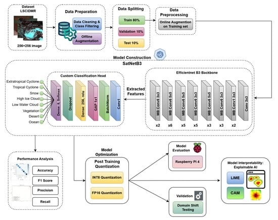
This section provides a detailed explanation of the workflow followed in this study, and Figure 1 summarizes the complete methodology. The process begins with acquiring the satellite imagery from the LSCIDMR dataset, followed by multiple preprocessing steps, including class filtering, the removal of underrepresented categories, and offline and online augmentation. After preparing the dataset, we develop the proposed SatNet-B3 architecture, which is an optimized version of EfficientNet-B3 tailored for satellite weather classification. The model is trained using the augmented dataset and validated with standard evaluation procedures. Finally, we apply post-training quantization techniques to convert the model into a lightweight INT 8 version for deployment on edge devices such as the Raspberry Pi 4. Figure 1 provides a high-level overview of these stages, and the subsequent subsections describe each component of this workflow in detail. Section 3.1 presents the data acquisition process and the characteristics of the LSCIDMR dataset. Section 3.2 explains the preprocessing pipeline. Section 3.3 introduces the proposed SatNet-B3 architecture. Section 3.4 discusses the post-training quantization techniques used to obtain the lightweight model, and finally Section 3.5 describes the deployment of the quantized model on the Raspberry Pi 4.

3.1. Data Acquisition and Description

Satellite data related to weather imagery were taken from the LSCIDMR dataset [29] obtained by the Himawari-8 satellite. The original dataset consists of 11 classes: Desert, Extratropical Cyclone, Frontal Surface, High Ice Cloud, Low Water Cloud, Ocean, Snow, Tropical Cyclone, Vegetation, Westerly Jet, and Label-less. These classes are grouped into three major meteorological categories: weather systems (Tropical Cyclone, Extratropical Cyclone, Frontal Surface, Westerly Jet, Snow), cloud systems (High Ice Cloud, Low Water Cloud), and terrestrial systems (Ocean, Desert, Vegetation), as defined in the original dataset [29]. The images are 256 × 256 pixels in size with a 10 min temporal resolution and 2 km spatial resolution. The dataset contains two types of annotations: single-label (LSCIDMR-S) and multi-label (LSCIDMR-M). The single-label images are classified based on the dominant scene type in the image, whereas the multi-label images are annotated with segmentations for each class in the image. For this study, LSCIDMR-S is chosen for image classification purposes.

Table 2. Brief descriptions of the meteorological and terrestrial classes in the LSCIDMR dataset.

Class	Brief Description
Tropical Cyclone	Low-pressure tropical vortex; distinct blue spiral cloud structure.
Extratropical Cyclone	Mid/high-latitude baroclinic cyclone with large cloud systems.
Frontal Surface	Boundary between contrasting air masses; elongated curved cloud belt forming a curved cyclonic structure.
Westerly Jet	Narrow high-altitude west–east wind band; thin streak-like appearance.
Snow	Surface ice-crystal coverage; darker textured appearance vs. high ice cloud.
High Ice Cloud	Cold high-altitude ice-crystal clouds (cirrus); blue-toned texture.
Low Water Cloud	Low-altitude warm water-droplet clouds; pink coloration in imagery.
Ocean	Large water bodies appearing dark or black in satellite images.
Desert	Arid sand-covered regions; light to dark brown appearance.
Vegetation	Land areas with plant cover; green-toned regions.
Label-less	Images without a dominant weather system, containing mixed or unclassifiable patterns.

provides a concise description of each class based on the visual and meteorological characteristics. Figure 2 presents one representative sample image from each class, except the Label-less category, to illustrate the visual differences between classes. Excluding the Label-less category, a total of 40,625 labeled images remain in the dataset. However, the remaining classes are highly imbalanced, as shown in Figure 3. For this reason, several data preprocessing steps are taken, as described in the following section.

3.2. Data Preprocessing

The original LSCIDMR data contain 11 categories (including the Label-less class). During dataset preparation, we removed the Label-less category (63,765 images), as it does not contain a dominant meteorological pattern, leaving a total of 40,625 labeled images that correspond to the remaining 10 meteorological classes defined in the dataset [29]. As shown in Figure 3, these classes are highly imbalanced. Within this labeled set, two categories, “Frontal Surface” and “Westerly Jet”, contain fewer than 1000 examples each.

As reported in [29], Frontal Surface and Westerly Jet occur far less frequently across seasons compared to other categories, resulting in substantially fewer labeled samples in the dataset. Due to this extremely limited representation, these classes provide insufficient data for stable supervised model training. Including classes with extremely few samples often leads to biased decision boundaries and unstable optimization during CNN training. Therefore, Frontal Surface and Westerly Jet were excluded from the final classification set.

After removing these two underrepresented classes, the final working dataset contains 39,363 images across the remaining eight categories. These eight classes cover all three major weather and surface types that the LSCIDMR authors identify as the primary scene categories in the dataset [29], and each retained class provides sufficient data for stable supervised learning. The adequacy of the retained classes was further confirmed by their clear visual distinction in sample images, a balanced distribution after augmentation, and the strong performance achieved by baseline CNN architectures during experimentation, indicating that the model was able to learn and differentiate each category effectively.

To improve generalization and increase intra-class variability, data augmentation techniques are carried out on the remaining dataset (39,363 images) to increase the number of samples and, hence, improve model performance and avoid overfitting. Offline augmentation techniques such as horizontal flip, rotation, shear, scale, blur, random brightness, contrast, and zoom are applied, which doubles the dataset to 78,726 images, and

Table 3. Offline image augmentation transformations.

Transformations	Setting
Horizontal Flip	Applied Randomly
Rotation	±10%
Zoom	±10%
Brightness Adjustment	±10%
Random Contrast	±0.2
Random Brightness	±0.2
Shear	−10° to +10°, 50% Probability
Scale	0.8 to 1.2, 50% Probability

shows the details of the transformations applied during augmentation. Figure 4 presents the class distribution before and after offline augmentation. The augmentation process increased the number of images in each class, providing a larger and more balanced dataset for training.

After offline augmentation, the dataset is split into training, validation, and test sets using an 80:10:10 ratio, respectively, and the final number of images in each split for all eight classes is summarized in

Table 4. Class-wise sample counts in the final dataset after splitting data into training, validation, and test sets (80:10:10).

Class	Train	Test	Val
Tropical Cyclone	5288	661	661
Extratropical Cyclone	7974	996	998
Snow	12,209	1526	1527
Low Water Cloud	2838	354	356
High Ice Cloud	8444	1055	1057
Vegetation	12,529	1567	1566
Desert	7230	903	905
Ocean	6467	808	809
Total	62,979	7870	7879

. Online augmentation techniques are applied only to the training set during model training to further reduce the impact of overfitting. These techniques include random horizontal flipping, random rotation, normalization, and resizing each image to a fixed resolution of 224 × 224 pixels. The images were normalized by adjusting their pixel values to a scale between 0 and 1, based on the mean and standard deviation for Z-score normalization. This step ensures that the pixel intensity values are standardized, following the equation below:

$$x_{\mathrm{normalized}}={\displaystyle \frac{x-{\mu }_x}{{\sigma }_x}}$$

(1)

where x denotes the original feature value prior to normalization. Here, ${\mu }_x$ represents the mean (average) of the values in the dataset or feature x, while ${\sigma }_x$ indicates the standard deviation of the values, reflecting the extent of variation from the mean.

3.3. Model Architecture

SatNet-B3 builds upon the EfficientNetB3 [30] architecture by incorporating a customized classification head and additional regularization techniques to enhance performance on an imbalanced and complex weather dataset.

Figure 5 illustrates the complete architecture of the proposed SatNet-B3 model, including the EfficientNet-B3 backbone and the custom classification head. The model receives a 224 × 224 × 3 satellite image as input and passes it through the stacked MBConv blocks of EfficientNet-B3. The model retains EfficientNet-B3’s pre-trained convolutional blocks for hierarchical feature extraction but incorporates several modifications in the classification head specifically designed to improve performance on imbalanced meteorological data. The feature map sizes across the backbone follow the original EfficientNet-B3 scaling rules, while the custom classification layers added in SatNet-B3 reshape and refine the extracted features to improve decision boundaries for satellite imagery.

EfficientNetB3 [30] is selected for its ability to balance high accuracy and computational efficiency, making it ideal for processing satellite weather imagery. The final classification stage of EfficientNet-B3 is removed with a custom classification head to refine the extracted deep features, followed by a BatchNormalization layer to stabilize training and improve convergence. A GlobalAveragePooling2D layer compresses the spatial dimensions and summarizes the feature maps into a compact vector, which is then fed into a Dense layer with 256 ReLU-activated units to learn high-level abstractions relevant to weather patterns.

To prevent overfitting and improve generalization, a Dropout layer with a 50% rate is added, randomly deactivating neurons during training. The final classification layer consists of a Dense layer with 8 units and a softmax activation function, which outputs a probability distribution over the classes. This streamlined architecture combines pre-trained feature extraction with custom layers to effectively classify weather patterns from satellite images.

Figure 6 provides a side-by-side comparison between EfficientNet-B3 and the proposed SatNet-B3. It illustrates the customized classification head of SatNet-B3, enabling the model to handle significant variations in cloud and surface patterns across the dataset, significantly improving the model’s ability to capture complex spatial patterns and variations in meteorological imagery. The effectiveness of this specific combination of custom layers is further validated in the ablation study (Section 4.4), where each architectural component is systematically evaluated and shown to contribute incrementally to the model’s final performance. After training the full-precision model, the final SatNet-B3 network was further optimized for deployment through post-training quantization, as detailed in Section 3.4.

3.4. Model Optimization

To improve deployment efficiency and validate SatNet-B3 as a lightweight architecture, post-training quantization was applied to reduce its computational footprint. The trained FP32 model was quantized using both the INT8 and Float16 optimization techniques. These approaches substantially reduced model size and inference time while maintaining comparable accuracy.

Table 5. The lightweight benchmarking of SatNet-B3 against its quantized variants and the second best-performing baseline model (Xception).

Model Type	Accuracy (%)	Inference Time (ms)	Model Size (MB)
SatNet-B3 (FP32)	98.22	20.42	128.7
SatNet-B3 INT8 quantized	98.20	103.51	11.6
SatNet-B3 FP16 quantized	98.21	74.66	21.3
Xception (FP32)	96.74	71.22	83.82

summarizes the performance of the original model, its quantized variants, and the Xception model, which is the second highest-performing architecture from the Xception model, which is the second highest-performing architecture among the evaluated baselines.

INT8 Quantization: Dynamic range INT8 quantization involves reducing the precision of weights and activations from 32-bit floating point (FP32) to 8-bit integers (INT8). During inference, most calculations are performed using 8-bit integers. However, the input and output layers are converted back to floating-point values to maintain precision. This approach significantly reduces memory usage and improves computational efficiency, making it ideal for deployment on edge devices. However, the reduction in precision can lead to a slight drop in model accuracy, which is observed in this study with a marginal decrease in accuracy from 98.22% to 98.20%, as shown in Table 5. This trade-off is generally acceptable when the primary goal is memory efficiency and faster inference times, especially for resource-constrained environments.

$$Q=\mathrm{round}\left({\displaystyle \frac{W}{S}}+Z\right)$$

(2)

where W represents the weight values, S is the scale factor, and Z is the zero point. These parameters map the FP32 values to the INT8 range $[-128,127]$. This approach resulted in a dramatic reduction in model size to 11.6 MB, which is a reduction of 90.98% in size, and an inference time of 103.51 ms, with a negligible drop in accuracy to 98.20%, as indicated in Table 5.

Float16 Quantization: Float16 quantization reduces the precision of model weights from FP32 to 16-bit floating-point (FP16) values. Unlike INT8 quantization, FP16 quantization maintains a higher dynamic range and precision for numerical computations, which is particularly advantageous for neural network architectures with sensitive floating-point operations. This method helps preserve model accuracy but does not achieve as significant a reduction in model size as INT8 quantization.

The transformation is expressed as follows:

$$W_{\mathrm{FP}16}=\mathrm{cast}(W_{\mathrm{FP}32},\mathrm{FP}16)$$

(3)

where $W_{\mathrm{FP}32}$ represents the original 32-bit floating-point weights, and $W_{\mathrm{FP}16}$ represents the converted 16-bit weights. This technique preserved the model’s accuracy at 98.21% while achieving a smaller model size of 21.3 MB and a faster inference time of 74.66 ms compared to the original FP32 model, as shown in Table 5.

To further validate the lightweight nature of SatNet-B3, a benchmarking experiment was conducted comparing the original FP32 model, its quantized variants, and the second highest-performing baseline model, Xception, as illustrated in Table 5. Post-training quantization substantially reduces the memory footprint of SatNet-B3, with INT8 compression reducing the model size from 128.7 MB to 11.6 MB, an overall 90% reduction, while FP16 reduces it to 21.3 MB. Since parameter tensors are stored in lower precision (8-bit or 16-bit), the effective parameter storage decreases proportionally, making the quantized versions significantly lighter. However, quantization does not reduce the number of parameters in the model; instead, it reduces the number of bits used to store each parameter, which decreases memory requirements while preserving the same architecture and capacity.

Despite this compression, SatNet-B3 maintains competitive accuracy (98.20–98.21%), outperforming the FP32 Xception baseline (96.74%) while requiring substantially less memory. Furthermore, SatNet-B3 achieves faster FP32 inference (20.42 ms) than the Xception baseline (71.22 ms), demonstrating that even before quantization, SatNet-B3 is inherently more efficient. These results collectively demonstrate that SatNet-B3 becomes highly lightweight after quantization, with INT8 quantization offering the most optimal balance between reduced model size, preserved accuracy, and practical inference performance for edge deployment.

3.5. System Implementation

The system is implemented by deploying the quantized SatNet-B3 onto a Raspberry Pi 4 (RPI4) for real-world testing and evaluation. This deployment provides an accurate representation of the model’s performance under actual hardware constraints.

Deploying deep learning models on embedded systems introduces several practical challenges that differ significantly from deployment on traditional high-performance computing platforms. Embedded devices such as the Raspberry Pi 4 have limited CPU power [31] and restricted memory [32], which reduce throughput, making it difficult to run large convolutional neural networks on computationally demanding image tasks in real time. Field deployments often operate under power and connectivity constraints [33,34,35], and environmental satellite data is collected in remote or resource-limited locations [36], making cloud-based solutions impractical for real-time weather analysis in remote regions. Techniques such as post-training quantization have been shown to reduce model size and computational requirements, enabling the deployment of convolutional neural networks on resource-constrained embedded devices such as the Raspberry Pi [37,38]. These constraints motivated the development of a lightweight architecture with post-training quantization to significantly reduce model size and computation cost. The proposed SatNet-B3 model directly addresses these challenges, enabling deployment on resource-constrained edge devices by reducing computational load, memory footprint, and energy consumption while maintaining accurate real-time performance.

Beyond addressing computational constraints, the choice of the Raspberry Pi 4 as the deployment platform is particularly well-suited for the requirements of this system. The Raspberry Pi 4 offers a practical trade-off of compute capability, memory, cost and ecosystem support for prototyping embedded ML applications [39,40]. Competing boards such as the Jetson Nano or Coral TPU offer higher peak performance [31], but they also draw more power during inference [39], exhibit higher thermal load under sustained workloads [41], and are typically more expensive than Raspberry Pi-class devices [39], which together reduce their practicality for low-power or budget-constrained field deployments [39]. Benchmarking studies further show that quantized CNNs achieve substantially lower inference latency and reduced computational load on Raspberry Pi-class devices [37,38,42], supporting their suitability for efficient embedded deployment. These characteristics directly support the objectives of this work, developing a lightweight, deployable, and cost-effective system for localized weather analysis that can operate in environments where traditional cloud or high-performance computing resources are unavailable.

With the improved computational capabilities of the RPI4, the model achieved an effective inference time of approximately 300 ms, demonstrating significant efficiency in processing satellite weather imagery. Figure 7 shows the Raspberry Pi 4 setup used for this deployment and on the device inference.

To support practical deployment, this work presents a system design for an edge-based satellite image analysis pipeline that integrates the quantized SatNet-B3 model with a Raspberry Pi 4 and an RTL-SDR module. The schematic diagram in Figure 8 illustrates the operational flow of this configuration, in which the hardware components follow standard, commercially available connections for embedded systems and are arranged to represent a realistic end-to-end pipeline for on-device classification. In this setup, a satellite antenna connects to the RTL-SDR via a dongle and coaxial cable. The RTL-SDR receives the signals when the satellite passes over and then decodes the image to the RPI4. Consequently, the image is then passed to the SatNet-B3 model for on-device weather classification. By integrating satellite signal acquisition (via RTL-SDR), onboard decoding, and quantized inference within a unified pipeline, the system design demonstrates that the proposed model can operate efficiently and reliably on low-power edge devices.

Power Consumption

It is important to consider the power requirements of the Raspberry Pi 4 when deploying models like SatNet-B3. Studies have shown that the Raspberry Pi 4 Model B consumes approximately 600 mA (3 W) when idle and up to 1.25 A (6.25 W) under the maximum stress with peripherals connected, such as a monitor, keyboard, mouse, and Ethernet [43]. Another study focusing on deep learning applications reported that running convolutional neural networks on a Raspberry Pi can lead to increased power consumption, correlating with model complexity and computational demands [44].

Based on these findings, the power consumption of SatNet-B3 during inference falls within the range of 3 W (idle) to 6.25 W (under load), which is consistent with the findings from benchmarking studies on edge devices running deep neural networks [31]. These values highlight the importance of appropriate power provisioning to maintain system stability and performance.

4. Results and Experimental Analysis

This section explores the comparative performance of various deep learning models including the proposed model. It illustrates the experimental setup and evaluation criteria used to assess the models, with particular attention to the proposed model’s efficiency and effectiveness.

4.1. Experimental Setting

This section compares the performance of several deep learning models, including the one proposed in this study. It details the experimental setup and evaluation criteria used to assess the models, with a special focus on the efficiency and effectiveness of the proposed model. The experimental setup follows the configuration described in

Table 6. Experimental environment for training models.

Environment	Configuration
CPU	Intel i7-12700 @2.10 GHz
GPU	GeForce RTX 3080
RAM	32 GB
OS	Windows 11 64-bit
Python	3.11

. Maintaining a consistent environment is important for making a fair and accurate comparison between the models. For model fine-tuning, we used libraries from TensorFlow, as they simplify the process of loading pre-trained weights and provide support for the preprocessing steps required during training.

4.2. Evaluation Metrics

In this study, the following evaluation metrics were used to assess model performance: accuracy, precision, recall, and F1 score.

Accuracy quantifies the overall correctness of the model by measuring the proportion of true outcomes (both true positives and true negatives) among all predictions. It is defined as follows:

$$\mathrm{Accuracy}={\displaystyle \frac{TP+TN}{TP+TN+FP+FN}}$$

(4)

where $TP$ denotes true positives, $TN$ denotes true negatives, $FP$ denotes False Positives, and $FN$ denotes False Negatives.

Precision focuses on the positive predictions made by the model, indicating the proportion of true positive predictions out of all predicted positives. The formula for precision is as follows:

$$\mathrm{Precision}={\displaystyle \frac{TP}{TP+FP}}$$

(5)

Recall, also known as Sensitivity, calculates the proportion of true positive results with respect to total actual positives. It is defined as follows:

$$\mathrm{Recall}={\displaystyle \frac{TP}{TP+FN}}$$

(6)

Finally, the F1 score provides a trade-off between precision and recall by computing their harmonic mean.

$$F1\mathrm{Score}=2·{\displaystyle \frac{\mathrm{Precision}·\mathrm{Recall}}{\mathrm{Precision}+\mathrm{Recall}}}$$

(7)

These metrics provide a comprehensive assessment of the model’s performance.

4.3. Achieved Results

In this study, 10 different CNN models were experimented with to evaluate their performance on the task. These models included commonly used architectures as well as the proposed SatNet-B3. Among them, SatNet-B3 delivered the best results, demonstrating superior precision, recall, F1 score, and accuracy compared to the other models. As presented in

Table 7. Comparison of different model architectures.

Model	Precision	Recall	F1 Score	Accuracy	Params (Millions)
ResNet50V2	0.9686	0.9573	0.9625	96.66	25.6
ResNet101	0.9413	0.9400	0.9394	94.48	44.7
MobileNetV2	0.9444	0.9422	0.9428	94.71	3.5
DenseNet121	0.9583	0.9513	0.9544	95.71	8.1
DenseNet201	0.9647	0.9585	0.9610	96.45	20.2
Xception	0.9636	0.9672	0.9653	96.74	22.9
InceptionV3	0.9644	0.9661	0.9652	96.70	23.9
InceptionResNetV2	0.9214	0.9133	0.9136	91.04	55.9
NASNetMobile	0.9249	0.9026	0.9111	91.33	5.3
SatNet-B3	0.9802	0.9809	0.9805	98.22	12.3

, SatNet-B3 achieved a precision of 0.9802, recall of 0.9809, F1 score of 0.9805, and an accuracy of 98.22%. These results show the effectiveness of SatNet-B3 in weather event classification, setting it apart from the other models evaluated.

The confusion matrix in Figure 9 shows that the model achieves strong classification performance across all eight classes, with most predictions lying on the diagonal. However, some minor misclassification can be seen. For instance, Desert is incorrectly predicted as Vegetation in 16 cases, and Snow is misclassified as Desert in 13 cases. These errors are primarily caused by high visual similarity in certain samples within these classes.

To better interpret these confusion trends, Figure 10 presents representative misclassified samples. As shown, Desert–Vegetation and Snow–Desert confusions arise due to overlapping visual patterns between these meteorological scenes in a single image. These examples highlight that inter-class overlapping exists in a small subset of the dataset, which contributes to the misclassification errors observed.

The ROC (Receiver Operating Characteristic) curve in Figure 11 plots the True Positive Rate against the False Positive Rate. The curves of models across its base, Float16, and INT8 formats were compared, denoting a good AUC value. Figure 12 presents the trade-off between precision and recall with an AUC greater than 0.99 among all classes.

4.4. Ablation Studies

To assess the impact of the custom layers added to the EfficientNetB3 backbone, an ablation study was conducted by progressively adding components and evaluating their performance. The results, shown in

Table 8. Comparison of model architectures and their performance. EB: EfficientNetB3 Base; TLF: Trainable Layers Frozen; TLU: Trainable Layers Unfreeze; GAP: Global Average Pooling Layer; Dense: Dense Layer; BN: Batch Normalization Layer.

Model	Precision	Recall	F1 Score	Accuracy
EB + TLF + GAP + Dense:8	0.8381	0.8238	0.8288	0.8505
EB + TLU + GAP + Dense:8	0.9315	0.8954	0.9078	0.9192
EB + TLU + GAP + Dense:256 + Dense:8	0.9760	0.9762	0.9761	0.9783
EB + TLU + GAP + BN + Dense:256 + Dense:8	0.9802	0.9809	0.9805	0.9822

, demonstrate the effectiveness of each layer combination.

Starting with the baseline model (EB + TLF + GAP + Dense:8), where the trainable layers are frozen, the performance is relatively limited. Unfreezing the layers (EB + TLU + GAP + Dense:8) improves the model’s flexibility, resulting in better performance. Further enhancement is observed with the addition of an extra Dense layer (EB + TLU + GAP + Dense:256 + Dense:8), which refines feature extraction, achieving an accuracy of 97.83%.

The inclusion of Batch Normalization (BN) and an extra Dense layer (EB + TLU + GAP + BN + Dense:256 + Dense:8) yields the best results, achieving a precision of 98.02%, recall of 98.09%, and an accuracy of 98.22%. These findings confirm that this particular combination of custom layers significantly enhances model performance by stabilizing training and improving convergence. This study highlights the importance of these modifications in optimizing the model’s classification capability.

To verify that these improvements were consistent, we additionally performed 5-fold cross-validation on the models. For each fold, models were trained using identical hyperparameters to assess stability across different data splits.

The averaged results are reported separately in

Table 9. Results of 5-fold cross-validation showing impact of different custom layer combinations on EfficientNetB3. Metrics are reported as mean ± standard deviation. EB: EfficientNetB3 Base; TLF: Trainable Layers Frozen; TLU: Trainable Layers Unfrozen; GAP: Global Average Pooling Layer; Dense: Dense Layer; BN: Batch Normalization Layer.

Model	Precision	Recall	F1 Score	Accuracy
EB + TLF + GAP + Dense:8	0.8211 ± 0.32	0.8142 ± 0.24	0.8183 ± 0.17	0.8311 ± 0.25
EB + TLU + GAP + Dense:8	0.8915 ± 0.12	0.8842 ± 0.10	0.8902 ± 0.11	0.8992 ± 0.15
EB + TLU + GAP + Dense:256 + Dense:8	0.9322 ± 0.13	0.9362 ± 0.76	0.9331 ± 0.61	0.9392 ± 0.32
EB + TLU + GAP + BN + Dense:256 + Dense:8	0.9539 ± 0.47	0.9502 ± 0.43	0.9553 ± 0.27	0.9568 ± 0.23

. The cross-validation results confirm that SatNet-B3 maintains strong and stable performance across different data splits.

4.5. Hyperparameter Analysis

The hyperparameter analysis process for the model focused on adjusting several key parameters, such as the optimizer, learning rate, and batch size.

Table 10. Hyperparameter analysis.

Optimizer	Learning Rate	Batch Size	Accuracy	F1
Adam	0.0005	16	0.9822	0.9805
Adadelta	0.001	32	0.7487	0.7271
SGD	0.005	16	0.9438	0.9392
RMSprop	0.0001	32	0.9799	0.9784
AdaGrad	0.01	32	0.9732	0.9716

provides a summary of the performance metrics, including accuracy and F1 score, for various optimizers and their corresponding parameter configurations. Among the optimizers tested, the Adam optimizer with a learning rate of 0.0005 and a batch size of 16 achieved the best performance, yielding an accuracy of 0.9822 and an F1 score of 0.9805. The results suggest that the selected combination of parameters for the Adam optimizer outperforms other optimizers such as Adadelta, SGD, RMSprop, and AdaGrad, as highlighted in the table. This analysis indicates that fine-tuning the hyperparameters is crucial for achieving optimal model performance in classifying satellite-based weather events.

4.6. Explainable AI

Explainable AI (XAI) has emerged in response to the increasing reliance on black-box models, making their decision-making more transparent. It includes various techniques that enhance the clarity and reliability of machine learning models, ensuring their outputs are comprehensible to humans. In image classification, it examines whether the model prioritizes meaningful regions, aligning with human perception. Common approaches for this include LIME and CAM.

4.6.1. LIME

LIME (Local Interpretable Model-Agnostic Explanations) is a technique that enhances model interpretability by providing explanations for individual predictions. It is model-agnostic, meaning that it can be applied to any supervised regression or classification model. LIME supports various data types, including images, text, and tabular data, making it a versatile tool for understanding machine learning decisions [45,46].

4.6.2. CAM

Class Activation Mapping (CAM) is an explainability technique used in convolutional neural networks (CNNs) to highlight image regions which are the most relevant to a model’s prediction. By generating heatmaps, CAM helps visualize which features contribute to classification decisions, improving interpretability [47].

In disaster image detection, CAM has been proven useful in detecting the most significant areas damaged by natural disasters, allowing for more transparent and trustworthy damage assessment. Its ability to highlight crucial regions guarantees that model judgments are consistent with human expert analysis, which increases trust in AI-powered disaster response systems [48,49].

4.6.3. Model Interpretability Using XAI

In this study, explainable AI techniques such as CAM and LIME were used to provide visual explanations for the model’s classification decisions. LIME highlights the edges that influenced the decision, while CAM generates heatmaps to indicate the key regions the model focused on. These techniques highlight the important features that influenced the model’s decision, showing that its classifications are based on the correct regions of the image, as shown in Figure 13.

4.7. Further Validation

The robustness and generalization capability of the proposed model are further examined by evaluating its performance on data with varying brightness levels and blurred images. A detailed discussion of the evaluation results for each method is provided in the following sections.

4.7.1. Brightness Adjustment

The model’s robustness to varying lighting conditions was evaluated by adjusting the brightness of the test images by ±20%. Despite these changes, the model retained its performance on both brighter and darker images, demonstrating its strong generalization ability under different illumination levels.

Table 11. Impact of brightness variation on model performance.

Model	Accuracy (%)
	Natural	Brighter (+20%)	Darker (−20%)
SatNet B3	98.22	97.73	97.92

reports the exact values achieved by the model with brightness adjustments, and Figure 14 presents examples of the images used in this evaluation, highlighting the variations in brightness.

4.7.2. Blurred Image Evaluation

The model’s ability to handle blurred inputs was assessed by evaluating its performance on images with varying levels of blur. Figure 15 presents examples of the images used in this evaluation. Despite increasing blur intensity, the model maintained high accuracy, which demonstrates its robustness to image degradation.

Table 12. Impact of blur variation on model performance.

Model	Accuracy (%)
	Natural	Blur (3×)	Blur (9×)	Blur (13×)
SatNet B3	98.22	98.02	97.86	96.90

presents the accuracies achieved under different blur levels.

5. Discussion

Table 13 presents a comparative analysis of recent works in weather classification using satellite imagery. Among these, the current state-of-the-art (SOTA) approach [16] utilized a snapshot-based residual network, SnapResNet152, achieving an accuracy of 97.25% on the LSCIDMR dataset. This dataset, as introduced in [29], also explored several architectures, including AlexNet, VGG-Net-19, ResNet-101, and EfficientNet, with an average accuracy of 92.475%, establishing a baseline for future work in weather classification using satellite imagery. Despite the strong performance of prior architectures, including the SOTA SnapResNet152, the proposed SatNet-B3 model surpasses these benchmarks, achieving an accuracy of 98.20% and establishing a new standard in weather classification using satellite imagery.

This improvement underscores the capability of the developed technique to classify high-resolution satellite images with enhanced precision, even under challenging conditions. By using the EfficientNetB3 backbone along with custom classification layers, SatNet-B3 effectively captures and extracts significant features from complex weather patterns, allowing it to distinguish between similar classes with greater accuracy. In addition, comprehensive data preprocessing and augmentation techniques were implemented to address the challenges posed by class imbalance and to enhance model generalization. Offline augmentation methods were used, which was complemented by online augmentation during training, which further reduced the risk of overfitting and improved the model’s robustness against diverse weather scenarios.

Furthermore, after quantization, the lightweight nature of SatNet-B3 distinguishes it from prior works. While many existing methods, including the use of SnapResNet152 [16], prioritize maximizing accuracy without considering deployment constraints, SatNet-B3 introduces a practical edge-oriented approach. Post-training quantization techniques (INT8 and Float16) significantly reduced model size and improved inference speed, making it suitable for embedded processing. The model was also successfully deployed on a Raspberry Pi 4, achieving an inference time of 0.3 s, which demonstrates its feasibility for real-time use in resource-limited environments.

Although weather-focused satellite image classification is an active research area, most existing studies focus on accuracy or segmentation quality and do not demonstrate real hardware deployment. As shown in Table 13, several weather-related methods [15,16,17,18,29] were evaluated exclusively on high-performance GPU systems, with no implementation on embedded or edge devices. In contrast, hardware-accelerated remote sensing systems that do report deployment [50,51,52] primarily address general land cover mapping or object detection rather than meteorological event classification, leaving real-time edge deployment in this specific domain largely unexplored.

Comparisons with these hardware-based remote sensing systems [50,51,52] further highlight this distinction. Unlike prior microcontroller-based platforms, which focus on broader remote sensing tasks, SatNet-B3 directly targets meteorological event classification while achieving substantially faster inference on low-cost hardware. This demonstrates a clear gap in the literature, and SatNet-B3 addresses this gap by providing the fastest reported implementation among weather-related satellite image classification, offering practical feasibility for operational meteorological applications.

Beyond its technical performance, this study emphasizes the interpretability of the model, which is important for meteorological applications. Explainable AI methods like LIME and Class Activation Mapping (CAM) were applied to show which parts of the satellite images had the greatest impact on the model’s classification decisions. This capability enhances the model’s reliability, particularly for critical scenarios like disaster management and agricultural planning.

Overall, the results demonstrate that SatNet-B3 not only surpasses the SOTA accuracy achieved by SnapResNet152 but also addresses the key limitations of prior works by effectively balancing performance, interpretability, and deployability. Its ability to handle high inter-class similarity and class imbalance while being optimized for lightweight deployment positions it as a robust solution for satellite-based weather image classification.

Table 13. Comparison of existing methods using satellite imagery.

Ref.	Dataset	Task	Model	Metrics	Implementation
[21]	CASID	Land cover semantic segmentation	SegNeXt	mIoU = 63.4%; Dice = 76.7%	-
[15]	Extreme-Weather	Spatiotemporal segmentation	Multichannel Spatiotemporal CNN	mAP = 52.92%	-
[17]	Kaggle Cloud Pattern Dataset	Cloud image segmentation	U-Net ResNet34	Dice Coeff = 0.662	-
[18]	INSAT-3DR	Cloud image segmentation and classification	Random Forest	Acc = 90%	-
[29]	LSCIDMR	Meteorological cloud image classification	AlexNet, VGGNet-19, ResNet101, EfficientNet-B5	Acc = 88.74%, 93.19%, 93.88%, 94.09%	-
[16]	LSCIDMR	Meteorological cloud image classification	SnapResNet152	Acc = 97.25%	-
[52]	DIOR dataset	Remote sensing object detection	YOLOv4-MobileNetv3	mAP = 82.61%	XilinxKV260 (FPS = 48.14)
[50]	NWPU-RESISC45 dataset, DOTA-v1.0 dataset	Remote sensing scene classification and aerial object detection	VGG16 & YOLOv2	Acc = 88.08%, 67.30%	Xilinx AC701 (VGG16 1.78 s, YOLOv2 17.12 s)
[51]	CubeSat	Cloud image segmentation	NU-Net	Acc = 90%	ESP32-CAM (6.1 s)
This Work	Modified LSCIDMR	Meteorological cloud image classification	SatNet-B3	Acc = 98.20%	Raspberry Pi 4 (0.3 s)

Table 13. Comparison of existing methods using satellite imagery.

Ref.	Dataset	Task	Model	Metrics	Implementation
[21]	CASID	Land cover semantic segmentation	SegNeXt	mIoU = 63.4%; Dice = 76.7%	-
[15]	Extreme-Weather	Spatiotemporal segmentation	Multichannel Spatiotemporal CNN	mAP = 52.92%	-
[17]	Kaggle Cloud Pattern Dataset	Cloud image segmentation	U-Net ResNet34	Dice Coeff = 0.662	-
[18]	INSAT-3DR	Cloud image segmentation and classification	Random Forest	Acc = 90%	-
[29]	LSCIDMR	Meteorological cloud image classification	AlexNet, VGGNet-19, ResNet101, EfficientNet-B5	Acc = 88.74%, 93.19%, 93.88%, 94.09%	-
[16]	LSCIDMR	Meteorological cloud image classification	SnapResNet152	Acc = 97.25%	-
[52]	DIOR dataset	Remote sensing object detection	YOLOv4-MobileNetv3	mAP = 82.61%	XilinxKV260 (FPS = 48.14)
[50]	NWPU-RESISC45 dataset, DOTA-v1.0 dataset	Remote sensing scene classification and aerial object detection	VGG16 & YOLOv2	Acc = 88.08%, 67.30%	Xilinx AC701 (VGG16 1.78 s, YOLOv2 17.12 s)
[51]	CubeSat	Cloud image segmentation	NU-Net	Acc = 90%	ESP32-CAM (6.1 s)
This Work	Modified LSCIDMR	Meteorological cloud image classification	SatNet-B3	Acc = 98.20%	Raspberry Pi 4 (0.3 s)

6. Conclusions

Accurately identifying weather events from satellite imagery is critical for disaster management and mitigating economic losses. This study introduced SatNet-B3, a quantized, lightweight deep learning architecture designed for the high-precision classification of satellite-based weather phenomena. It utilized EfficientNetB3 as the backbone with custom classification layers, and SatNet-B3 achieved a state-of-the-art accuracy of 98.20% on the LSCIDMR dataset, surpassing the existing benchmarks. The model was further enhanced through comprehensive data preprocessing and augmentation methods, effectively addressing challenges like class imbalance and high inter-class similarity.

To optimize deployment feasibility, post-training quantization techniques, including INT8 and Float16 formats, were applied, reducing the model size and inference time. The successful deployment of SatNet-B3 on a Raspberry Pi 4 device, where it achieved an inference time of 0.3 s, validates its suitability for real-world applications in resource-constrained settings. Explainable AI techniques, such as LIME and Class Activation Mapping (CAM), were used to show the areas in satellite images that had the greatest impact on the model’s classification decisions. This improves the model’s interpretability and enhances its reliability, particularly for critical meteorological applications.

While SatNet-B3 demonstrates strong potential for weather classification, several limitations remain. Although the model shows robustness against brightness variations and multiple levels of blur, it has not been evaluated under more challenging real-world conditions that frequently occur in satellite imagery, such as extreme haze, heavy cloud cover, sensor noise, or compression artifacts. Moreover, the dataset primarily represents a specific range of atmospheric conditions, so generalization to other seasons, geographic regions, or different satellite sensors remains to be validated. From a computational perspective, although INT8 quantization improves inference efficiency, deployment on low-power devices such as the Raspberry Pi 4 is still constrained by limited CPU throughput, which restricts performance for high-resolution or continuous-stream inputs. Furthermore, the final experiments were conducted on eight of the ten labeled meteorological classes in the LSCIDMR dataset. The “Frontal Surface” and “Westerly Jet” categories were excluded due to their substantially smaller sample sizes, which introduced severe class imbalance and instability during supervised training. Although the remaining eight classes span all three major meteorological systems and focus on the most well-represented categories, this exclusion limits the model’s coverage of rare meteorological events.

Addressing these limitations will be an important direction for future work. Future efforts could involve expanding the system’s deployment to integrate physical antenna systems for direct real-time data acquisition, testing the model on various edge devices beyond the Raspberry Pi 4 to assess environment-specific performance. Additionally, the deployment of the system on boats or ships for real-time data collection and weather analysis could greatly improve safety and preparedness for sea travelers. Further improvements may focus on additional compression techniques, broader evaluation across diverse imaging conditions, and integration with live-weather systems in disaster-prone regions. Evaluating SatNet-B3 on data from different satellites can also enhance its generalizability. Future research may also explore targeted data collection to reintegrate rare categories, such as the Frontal Surface and Westerly Jet categories, and expand the model’s applicability to a broader range of meteorological events. Overall, this research has the potential to improve weather analysis systems and enhance disaster preparedness in resource-limited settings.