QL-AODV: Q-Learning-Enhanced Multi-Path Routing Protocol for 6G-Enabled Autonomous Aerial Vehicle Networks

Abstract

With the arrival of sixth-generation (6G) wireless systems comes radical potential for the deployment of autonomous aerial vehicle (AAV) swarms in mission-critical applications, ranging from disaster rescue to intelligent transportation. However, 6G-supporting AAV environments present challenges such as dynamic three-dimensional topologies, highly restrictive energy constraints, and extremely low latency demands, which substantially degrade the efficiency of conventional routing protocols. To this end, this work presents a Q-learning-enhanced ad hoc on-demand distance vector (QL-AODV). This intelligent routing protocol uses reinforcement learning within the AODV protocol to support adaptive, data-driven route selection in highly dynamic aerial networks. QL-AODV offers four novelties, including a multipath route set collection methodology that retains up to ten candidate routes for each destination using an extended route reply (RREP) waiting mechanism, a more detailed RREP message format with cumulative node buffer usage, enabling informed decision-making, a normalized 3D state space model recording hop count, average buffer occupancy, and peak buffer saturation, optimized to adhere to aerial network dynamics, and a light-weighted distributed Q-learning approach at the source node that uses an ε-greedy policy to balance exploration and exploitation. Large-scale simulations conducted with NS-3.34 for various node densities and mobility conditions confirm the better performance of QL-AODV compared to conventional AODV. In high-mobility environments, QL-AODV offers up to 9.8% improvement in packet delivery ratio and up to 12.1% increase in throughput, while remaining persistently scalable for various network sizes. The results prove that QL-AODV is a reliable, scalable, and intelligent routing method for next-generation AAV networks that will operate in intensive environments that are expected for 6G.

1. Introduction

The rapid evolution of sixth-generation (6G) mobile networks is unlocking unprecedented opportunities for the deployment of autonomous aerial vehicle (AAV) systems in critical applications such as security surveillance, emergency rescue, and temporary telecommunications services [1,2]. By offering sub-millisecond ultra-low latency, terabit-per-second bandwidth, and an inherently AI-native architecture, 6G provides an ideal foundation for orchestrating large-scale AAV swarms operating in three-dimensional space. Yet the design and implementation of efficient routing protocols for AAV networks under 6G conditions remain highly challenging owing to the network’s extreme topological dynamics, stringent energy constraints, and rigorous quality-of-service (QoS) requirements [3]. Within the 6G context, AAV swarms are expected to function as intelligent, distributed systems with massive connectivity, enabling hundreds or even thousands of vehicles to coexist in confined airspace [2].

The AI-native architecture of the 6G network essentially changes the operational functionality of AAVs by moving intelligence to the edge [4]. Distributed intelligence not just allows for real-time processing and decision-making close to the source but also permits AAVs to learn from their environment constantly and dynamically adapt to complex, uncontrollable situations. Such adaptability becomes a necessity in leveraging cutting-edge machine learning frameworks, particularly reinforcement learning (RL), in optimizing routing, navigation, and task allocation policies in highly dynamic airspace environments [5]. Moreover, the ultra-low-latency and high-reliability requirements defined by 6G standards render traditional routing protocols, inherently with terrestrial mobile network origins, unfit for aerial vehicular networks. These conventional approaches are typically unable to offer the real-time response, scalability, and flexibility needed by 6G-based applications. Therefore, there is an immediate need to redesign or revamp current routing protocols by integrating AI-driven decision engines with real-time optimization, predictive analytics, and context-aware communication strategy to offer seamless connectivity, low delay, and robust QoS in varying flight conditions [6,7,8].

One of the foremost challenges in designing AAV routing protocols is the vehicles’ high mobility, with velocities reaching up to 460 km/h in three-dimensional flight [8]. Unlike conventional mobile networks confined mainly to a two-dimensional plane, an AAV network experiences continuous topological changes in all three spatial dimensions, resulting in frequent link disruptions and difficulties in maintaining stable routes. Additionally, AAVs face strict energy limitations due to finite battery capacity, requiring routing protocols to treat energy efficiency as a critical path-selection criterion [9]. Real-time decision-making further compounds the problem, as AAVs must continuously update and adjust routing choices within extremely short time windows to uphold service quality.

The standard ad hoc on-demand distance vector (AODV) protocol, although widely adopted in mobile ad hoc networks, suffers significant drawbacks when applied to AAV networks in a 6G environment [10]. AODV maintains only a single route per destination and lacks the ability to learn from past routing experiences, leading to poor performance under highly dynamic conditions. Moreover, AODV disregards congestion information at intermediate nodes and along entire routes, which diminishes overall system efficiency. To overcome these limitations, this work proposes the Q-learning-enhanced AODV (QL-AODV) protocol. This novel routing scheme embeds RL capability into AODV to optimize routing decisions based on experiential knowledge gleaned from the network environment. The main contributions of this work are as follows.

• Design of an intelligent multipath-collection mechanism. This work proposes a scheme that stores and simultaneously evaluates up to ten candidate routes per destination by extending the route reply (RREP) waiting window, thereby generating a rich dataset for learning and optimal path selection.
• Extension of the RREP packet format. The proposed work redesigns the RREP from 19 bytes to 27 bytes by adding two critical fields, total buffer occupancy and maximum buffer occupancy, enabling efficient congestion information gathering along the entire route.
• Construction of an AAV-oriented state space. The proposed model defines a three-dimensional state vector that combines hop count, average buffer occupancy, and maximum buffer occupancy, each normalized to the range [0, 1] to ensure learning-algorithm stability.
• Integration of Q-Learning into the AODV protocol.

The remainder of this paper is organized as follows: Section 2 reviews related work on AAV routing protocols and machine-learning applications in routing. Section 3 presents the proposed QL-AODV protocol, including the AAV network model, detailed protocol design, Q-Learning components, operational workflow, and specific algorithms. Section 4 evaluates the performance through comprehensive NS-3 simulations and comparative analysis. Finally, Section 5 concludes the paper and discusses future research directions.

2. Related Works

AAV networks comprise self-organizing, self-configuring aerial platforms that maneuver continuously in three-dimensional space. Their salient characteristics include high mobility, rapidly fluctuating topologies, stringent energy constraints, and demanding QoS requirements, namely ultra-low latency, high throughput, and strong reliability [11]. Figure 1 presents the AAV topology with buffer occupancy levels. Traditional routing protocols such as optimized link state routing (OLSR), dynamic source routing (DSR), and AODV have been widely adopted in wireless ad hoc networks; however, each exhibits pronounced limitations when transplanted to AAV scenarios [10,12]. OLSR maintains a complete topological view by persistently disseminating control traffic, which inflates signaling overhead, especially as node count and velocity escalate [13]. The resultant control burden wastes scarce resources, accelerates energy depletion, and curtails network lifetime; moreover, frequent updates introduce additional latency and depress throughput in highly dynamic environments.

DSR, an on-demand protocol that stores entire source routes in every data packet, can rapidly reconstruct paths and minimize route-discovery delay in small-scale networks. Yet under the high-speed mobility of AAVs, where links change incessantly, this strength becomes a liability. The continuous updating and carriage of complete path information markedly enlarge packet size, consuming bandwidth and reducing energy efficiency. At the same time, stale cached routes quickly become invalid, heightening packet-loss risk and necessitating perpetual rediscovery. DSR protocols are inherently unsuitable for highly dynamic and large-scale aerial networks, where topological instability and node density are at their extreme. The unscalability of routes becomes a bottleneck with increasing hops, and the route maintenance overheads become recurrent [14].

Moreover, source routing imposes a centralized decision-making model, which contradicts the decentralized, edge-intelligent nature of modern 6G-equipped AAV systems. This centralization hinders real-time responsiveness and subjects the system to single points of failure [15]. Furthermore, the overhead of maintaining large route caches and disseminating frequent route requests can lead to network congestion, particularly when many AAVs are airborne at the same time in overlapping coverage areas. As a result, DSR protocols do not offer high-reliability and low-latency communication and hence cannot be employed for mission-critical use cases such as autonomous swarming, surveillance, and emergency response in 6G-enabled aerial networks.

AODV, another on-demand mainstay, discovers and maintains routes only when required. Although effective in moderately dynamic terrestrial ad hoc networks, AODV reveals critical shortcomings in AAV contexts. First, it sustains only a single route per destination, a rigidity ill-suited to highly volatile environments that demands swift and efficient path recovery. Second, it lacks adaptability to fast-changing conditions such as congestion, often selecting routes sub-optimal in terms of delay and throughput. Finally, AODV disregards network-state indicators (e.g., buffer occupancy or congestion) when making routing decisions, significantly undermining performance in dense, highly dynamic AAV deployments [16,17].

Godfrey et al. [18] replaced AODV’s hop-count heuristic with a model-free RL agent that runs in the SDN controller. Each switch reports queue length, link reliability, and hop count; these features form the state fed to a Q-learning module that chooses the next hop to bypass incipient congestion. A “look-ahead” update propagates rewards two hops ahead, enabling the policy to react before buffers overflow. By decoupling control from data and learning from live feedback, QCAR turns routing into a proactive congestion-avoidance task rather than a reactive path-repair one, making it suitable for highly dynamic, centrally managed backbones.

B. M. El-Basioni [19] conducted an exhaustive design-of-experiments paper on plain AODV in a fully mission-controlled drone network, then derived a recommended “AAV networks operational environment (FAODVN-OE)”. The contribution is not a new algorithm but a systematic approach. It achieved smaller TTLs to curb flooding, longer ACTIVE_ROUTE_TIMEOUT to mask transient breaks, and a selective HELLO mechanism invoked only when topology volatility warrants it. The outcome is an AODV variant that pursues jitter and delay minimization for data-collection swarms without redesigning packet formats, reflecting a “tune-before-revise” philosophy.

X. Li et al. [20] proposed the CND-AODV approach using the idea of neighboring node (ND). Each node computes the count of neighbors it shares with the RREQ sender (common-neighbor density) and uses a z-score test to decide whether to rebroadcast. By factoring in topological context instead of raw degree, the model preserves essential relays while still throttling excess floods. The protocol, therefore, positions itself as a topology-aware, storm-mitigating enhancement that seeks to balance overhead, delivery ratio, and delay across diverse mobility and density patterns. Chandrasekar et al. [21] targeted the security of flying ad hoc networks rather than performance. They embed a lightweight trust engine into the AODV. Nodes score one another using direct packet-forward observations and indirect recommendations maintained by a central controller. During route discovery, hops whose trust value falls below a dynamic threshold are excluded, and detected attackers are blackholed from future RREQ and data forwarding. The model’s core innovation is joint routing-and-reputation coupling that filters false identities and black-hole attacks without expensive cryptography.

Dong et al. [22] extended the AODV approach with two composite metrics: residual-energy balanced by node degree, and relative mobility between successive hops. During RREP collection, the source computes a cost that weights both factors, then selects the path that equalizes energy drain and maximizes link stability. By shifting from “shortest path” to “lifetime-aware stable path”, AODV-EM aims to sustain network connectivity in dense, high-speed AAV swarms where key nodes tend to die early or break links frequently. An analysis of the related literature reveals the following three principal limitations when these schemes are applied to AAV networks.

(1)

An inability to exploit multipath diversity: approaches such as ND-AODV and CND-AODV still adhere to the single-path selection strategy of legacy AODV.

(2)

The absence of distributed adaptive learning: QCAR adopts a centralized Q-learning model that conflicts with the self-organizing nature of AAV networks, whereas FAODVN-OE and AODV-EM merely adjust static parameters.

(3)

Insufficient global network-state visibility: existing methods consider only local information or a single metric, ignoring congestion conditions along the entire route.

To overcome these shortcomings, this work proposes the QL-AODV protocol, which fuses distributed Q-learning with an intelligent multipath-collection mechanism. Specifically, the proposed QL-AODV lengthens the RREP waiting interval to assemble a candidate-route set and augments the RREP format to carry cumulative buffer-occupancy information along the path. The Q-learning state vector is expressly designed for AAV environments, combining hop count, average congestion level, and maximum congestion level, each normalized to the [0, 1] range. Q-learning is selected for its model-free nature and online-learning capability, both of which align with the high dynamism of AAV networks.

3. Proposed Q Learning AODV Protocol

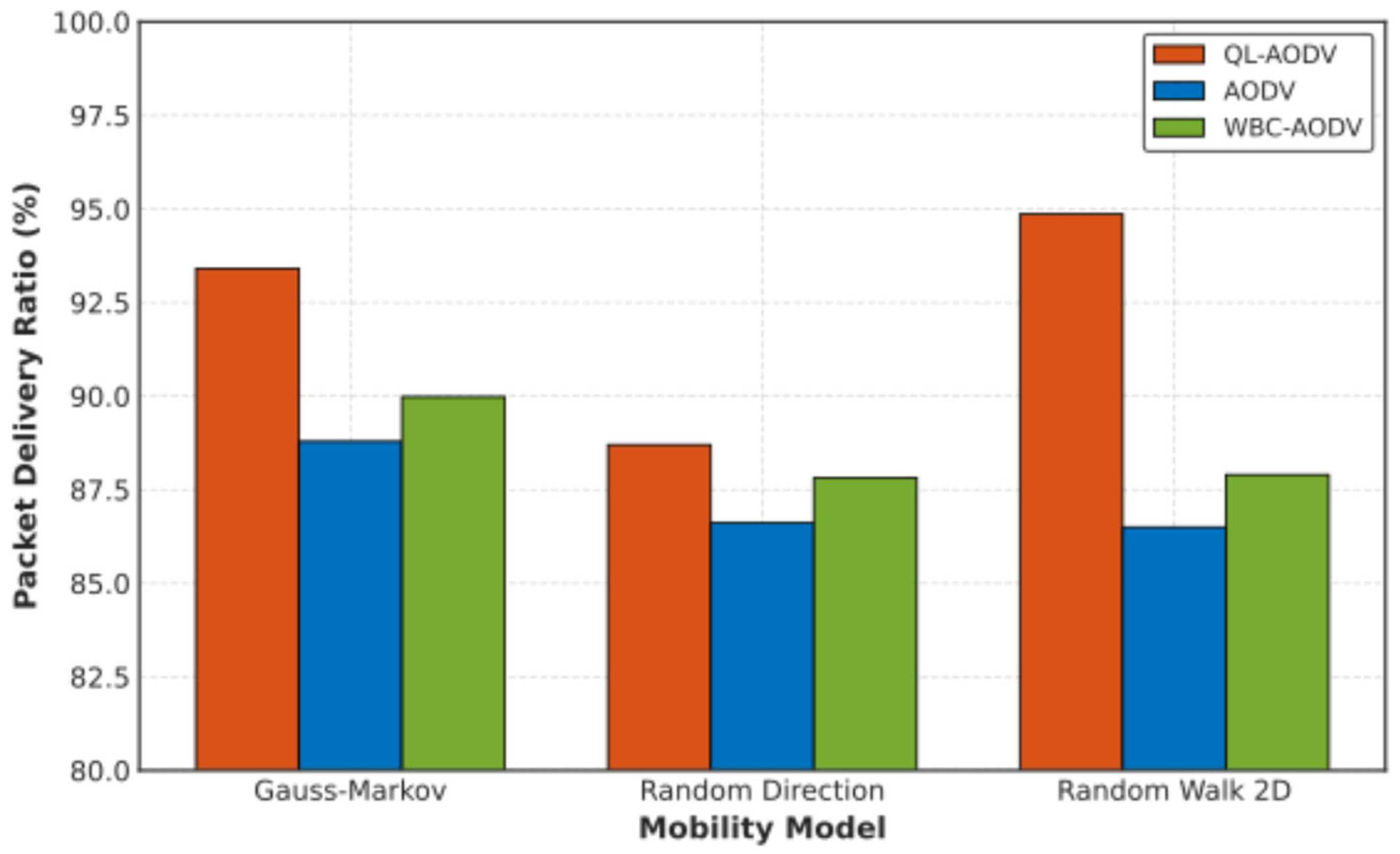
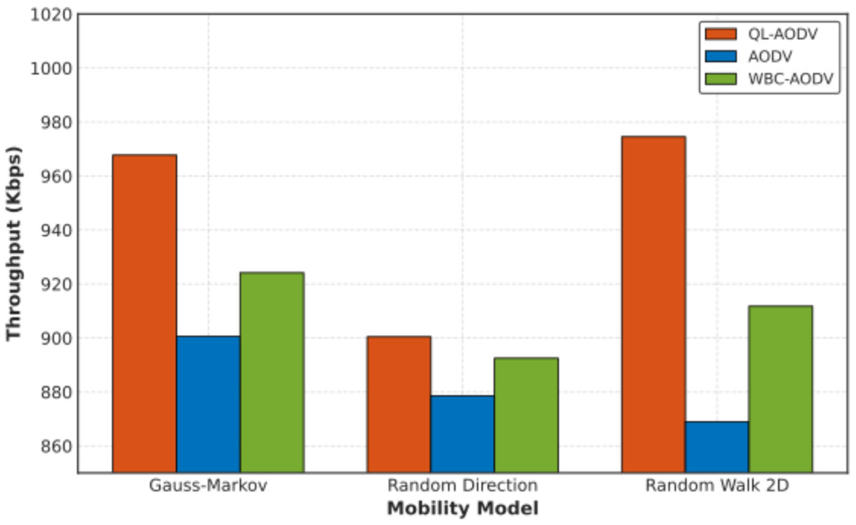
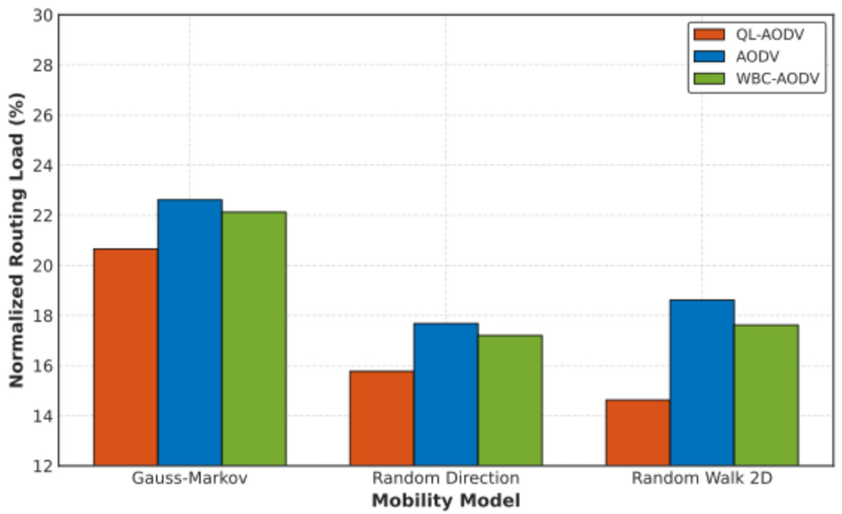
This section presents the proposed Q-learning AODV (QL-AODV) routing protocol for AAV networks. It begins by describing the AAV network model and then summarizes the main features of the baseline AODV protocol. Next, the detailed design of QL-AODV is introduced, including the extended packet structure, the core components of the Q-learning algorithm, the overall operational workflow, and the specific algorithms employed.

3.1. AAV Network Model

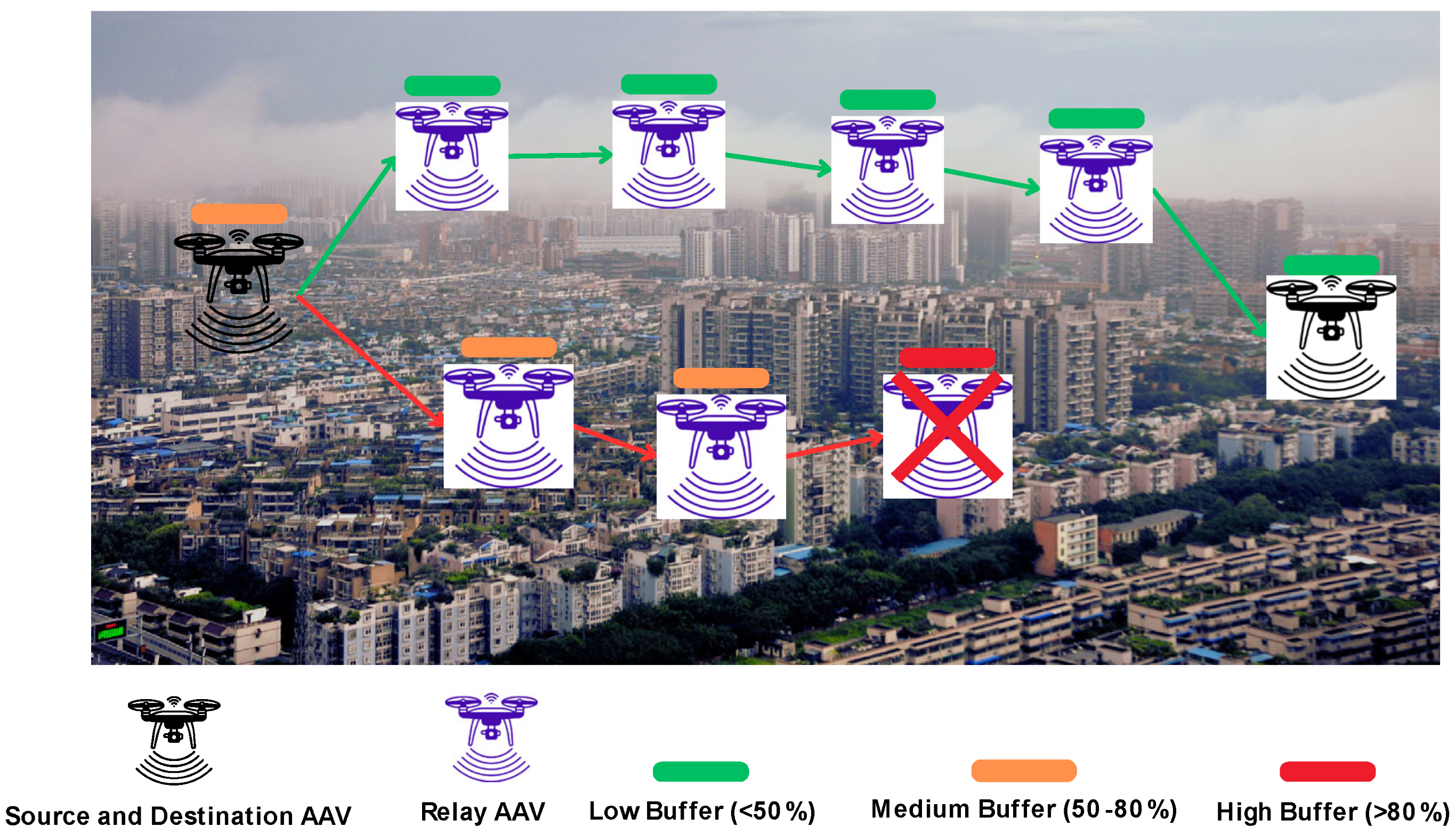
The network under consideration consists of a set of AAVs, NAAV, operating within a defined three-dimensional space to conduct cooperative tasks such as surveillance, data collection, or communication support. These AAVs form a flying ad hoc network in which every vehicle is self-organizing and self-configuring and functions as a network router. The AAV topology is highly dynamic owing to continuous movement, which causes rapid variations in inter-node connectivity. Each AAV is equipped with a wireless interface and can communicate with its peers (AAV-to-AAV, U2U) and with the base station (AAV-to-base station, U2B) within a given transmission range. Every AAV maintains a buffer for packets awaiting forwarding. The network operates in a 6G context that promises wide bandwidth, low latency, and native AI integration, and can interact with fog-computing nodes to enhance processing capacity and reduce latency for delay-sensitive applications.

The AAV network is modeled as a time-dependent undirected graph $G\left(t\right)=\left(V\right(t),E(t\left)\right)$, where V(t) represents the set of AAVs and base stations at time t, and E(t) denotes the set of wireless links between nodes that lie within mutual transmission range. The proposed QL-AODV algorithm is built on the AODV routing framework and incorporates RL via Q-learning to optimize path selection. The principal enhancements include an extended RREP packet that conveys additional network-state information, the definition of Q-Learning components, and modifications to the route-selection procedure.

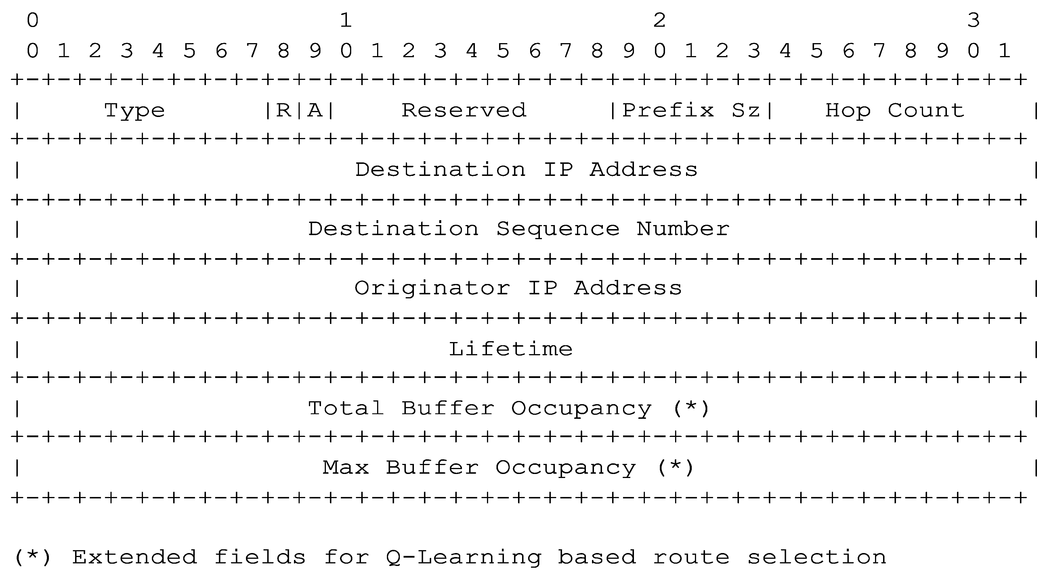
Figure 2 presents the proposed extended RREP packet format for the proposed QL-AODV. To provide visibility into potential congestion along a route, we extend the AODV RREP structure. Based on the implementation in aodv-packet.h (class RrepHeader) and aodv-packet.cc, two new fields are added.

(1)

uint32_t m_totalBuffer

Stores the total buffer occupancy aggregated over all nodes from the RREP originator (destination or intermediate) back to the source. The unit may be the number of packets or a percentage. In the proposed implementation, (aodv-routing-protocol.cc, function GetBufferOccupancy) represents queue occupancy in percentage.

(2)

uint32_t m_maxBuffer

Stores the maximum buffer occupancy observed at any node along the route.

When a node (destination or intermediate) generates an RREP, it initializes these fields with its own buffer information. As the RREP propagates back to the source, each intermediate node updates the fields as follows.

• localBuffer = GetBufferOccupancy()
• RREP.total_buffer = RREP.total_buffer + localBuffer
• RREP.max_buffer = MAX(RREP.max_buffer, localBuffer)

To enable buffer-aware routing decisions, we extend the standard AODV RREP message format from 19 bytes to 27 bytes. This means that when the source node receives an RREP, it holds aggregated buffer information for the entire route, enabling more intelligent path selection. The new RREP is eight bytes larger than its legacy AODV counterpart. To quantify congestion for QL-AODV routing decisions, we measure the occupancy of the AODV routing queue (RequestQueue) using a sliding time window. Each node updates two windowed statistics in the background, expressed as a percentage of queue capacity: the windowed mean ${\mu }_{\mathrm{buf}}$ and the windowed maximum ${\mathrm{m}\mathrm{a}\mathrm{x}}_{\mathrm{buf}}$. When an RREP traverses a node, the node reads these pre-computed values and writes them into the header field for aggregation along the path. At the source, the path-mean and path-maximum are normalized to $[0,1]$ (avgBufNorm and maxBufNorm) and used as the Q-learning state. This design suppresses instantaneous noise from micro-bursts, preserves sensitivity to short congestion peaks, and adds no control-plane latency, since all computations run periodically in the background.

Our QL-AODV implementation monitors the AODV routing buffer (RequestQueue) rather than the MAC layer transmission buffer. The AODV routing buffer stores packets awaiting route discovery at the network layer, while the MAC buffer stores packets with established routes awaiting channel access. We focus on AODV buffer occupancy because: (1) it directly reflects routing protocol performance issues, (2) its congestion triggers costly route rediscovery processes in high-mobility UAV networks, and (3) it provides actionable information for routing optimization decisions. The buffer occupancy fields in our extended RREP format (m_totalBuffer and m_maxBuffer) specifically measure the percentage occupancy of AODV routing queues, enabling intelligent congestion-aware route selection.

3.2. Q-Learning Components

Q-Learning is a model-free, off-policy RL algorithm that seeks to learn an action-value function, denoted $Q(s,a)$, estimating the expected cumulative reward obtained by performing the action $a\in \mathcal{A}$ in state $s\in \mathcal{S}$. Within the proposed QL-AODV framework, the main Q-Learning components are defined as follows.

(a)

State space (δ)

A state characterizes the quality of a potential route from the source to the destination, constructed from information carried in the RREPs received at the source. Specifically, s is a normalized three-tuple.

$$s=(h_{\mathrm{norm}},\hspace{0.17em}{b}_{\mathrm{avg}\_\mathrm{norm}},\hspace{0.17em}{b}_{\max \_\mathrm{norm}}),$$

(1)

where h_norm is the normalized hop count, b_{avg_norm} is the normalized average buffer occupancy along the route, and b_{max_norm} is the normalized maximum buffer occupancy of any node on the route. The normalized hop count (h_norm) is the hop count h to the destination, normalized by a constant. It can be calculated as follows with $H_{\max }=10$.

$$h_{\mathrm{norm}}={\displaystyle \frac{h}{H_{\max }}},$$

(2)

The normalized average buffer occupancy along the route (b_{avg_norm}) is obtained by dividing the cumulative buffer occupancy B_total (field m_total-Buffer in the RREP, i.e., the sum of per-node occupancy percentages) by the hop count h and normalized by the maximum node buffer occupancy B_{node_max%}. It can be calculated as follows.

$$b_{\mathrm{avg}\_\mathrm{norm}}={\displaystyle \frac{B_{\mathrm{total}}}{h\cdot B_{\mathrm{node}\_\max \%}}},$$

(3)

The normalized maximum buffer occupancy of any node on the route (b_{max_norm}) is given as follows.

$$b_{\max \_\mathrm{norm}}={\displaystyle \frac{B_{\max \_\mathrm{val}}}{B_{\mathrm{node}\_\max \%}}},$$

(4)

where B_{max_val} is taken from the m_maxBuffer field of the RREP. Normalization confines all state components to $\left[\mathrm{0,1}\right]$, placing them on a standard scale and thereby enhancing learning stability and efficiency.

(b)

Action space $\mathrm{(𝒜}$)

If the source collects multiple RREPs for the same destination during the interval $T_{\mathrm{wait}}$, it forms a set of candidate routes $P_{\mathrm{routes}}=\{p_1,p_2,\dots ,p_k\}$ with $k\le K_{\max }=10$. Each route $p_i$ is identified by an index $i{d}_i$ (0 … $K_{\max }-1$). An action $a\in \mathcal{A}$ corresponds to selecting a route $p_a$. For data forwarding, the action space is $\mathcal{A}=\{a_0,a_1,\dots ,a_{K-1}\}$.

(c)

Reward function (R)

The reward $R(s,a)$ quantifies the immediate effectiveness of choosing an action $a$ (route $p_a$) in the state $s$. The proposed QL-AODV employs a simple binary reward as follows.

$$R(s,a)=\left\{\begin{array}{ll}+1,& \mathrm{if} \mathrm{the} \mathrm{packet} \mathrm{is} \mathrm{successfully} \mathrm{transmitted} \mathrm{over} p_a\\ -1,& \mathrm{if} \mathrm{the} \mathrm{transmission} \mathrm{over} p_a \mathrm{fails}\end{array}\right.,$$

(5)

Determining “success” or “failure” is crucial. In hop-by-hop AODV routing, success can be defined as receiving a MAC-layer acknowledgement (IEEE 802.11 MAC ACK) for a packet forwarded to the next hop. Conversely, failure is recorded when the MAC layer reports a transmission error, or no ACK is received within a specified timeout. This binary outcome supplies the Boolean success input to the UpdateQValue function in the implementation.

(d)

Q-value update rule

The action-value $Q(s,a)$, denoting the expected cumulative reward obtained by acting $a$ in state $s$ and thereafter, following the optimal policy, is iteratively updated through the Bellman equation.

$$Q_{k+1}\left(s,a\right)=Q_k\left(s,a\right)+\alpha \left[R\left(s,a\right)+\gamma {\mathrm{m}\mathrm{a}\mathrm{x}}_{a^{\prime }}{Q}_k\left(s^{\prime },a^{\prime }\right)-Q_k\left(s,a\right)\right] \forall 0<\alpha \le 1, 0\le \gamma <1,$$

(6)

where k is the learning-iteration index, α is the learning rate, γ is the discount factor, s is the current system state before choosing an action $a$, $s^{\prime }$ is the next system state after the action $a$ is executed, and ${\mathrm{m}\mathrm{a}\mathrm{x}}_{a^{\prime }}{Q}_k(s^{\prime },a^{\prime })$ is the maximum estimated Q-value in state $s^{\prime }$, obtained by selecting the optimal action $a^{\prime }$.

In the proposed implementation, the term (maxNextQ) is computed by scanning the largest Q-values of all feasible actions from the candidate states associated with the destination under consideration. The Q-table, which stores the values $Q(s,a)$, is implemented as a “nested std::map”; the outer key is the destination’s IP address, the inner key is a QState object (hashed via QStateHash for use in std::unordered_map), and the final value is a std::vector<double> in which each element corresponds to the Q-value of an action (a routeId) available from that state.

3.3. Operational Process of the QL-AODV

A.

Phase 1—Route Discovery and Information Collection

The first phase of the proposed QL-AODV algorithm begins when a source node (S) has data to transmit to a destination node (D) without having a valid route. In such a case, S initiates a route request (RREQ) broadcast similar to the regular AODV protocol. This RREQ propagation is used to search current paths to the destination by traversing the network. Whenever the RREQ packet is forwarded from one intermediate node to another, the destination node constructs a fresh reverse route or updates an old one to the source node. In the situation where an intermediate node possesses a valid and sufficiently fresh route to the destination D (the “Destination Only” flag having been cleared), or in the situation where the node is the destination itself, it replies by sending a RREP packet.

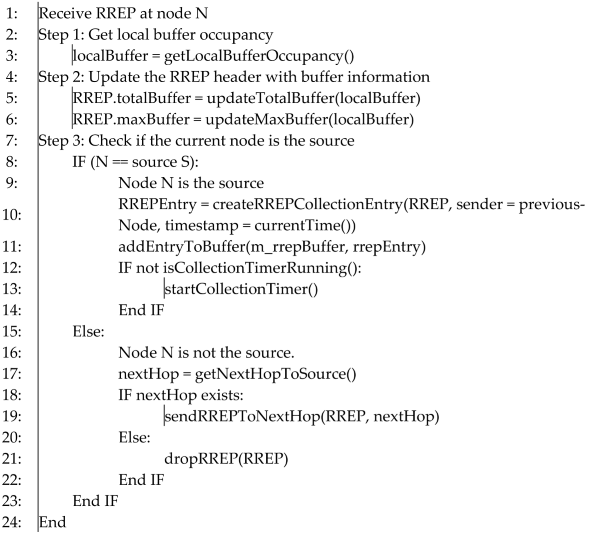
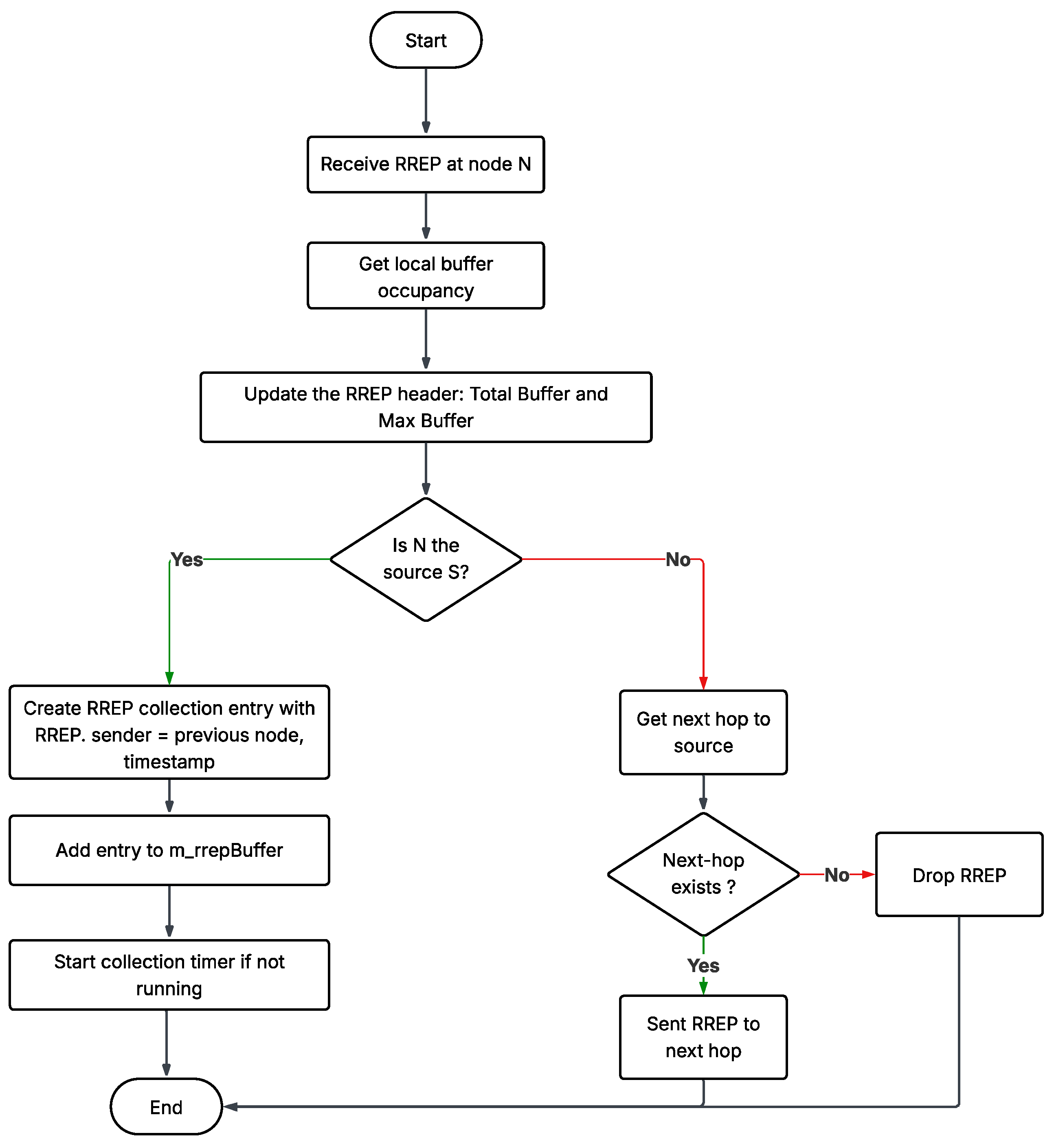
At this stage, the RREP originator node, denoted as Nrrep, initiates buffer-awareness by placing its own buffer usage statistics in the RREP stream. Specifically, it places the values of m_totalBuffer and m_maxBuffer, indicating its current buffer state. With the RREP being forwarded back towards the source node in the reverse direction, each forwarding intermediate node (N_int) makes contributions to the buffer data aggregation. It does so by retrieving its local buffer occupation, localBuffer = N_int.GetBufferOccupancy(), and assigning the RREP fields accordingly. The sum buffer field (RREP.m_totalBuffer) is added with localBuffer, and the max buffer field (RREP.m_maxBuffer) is assigned to hold the maximum value achieved up to that point.

Finally, upon receiving RREPs from various paths, source node S remains idle for a fixed amount of time, i.e., m_rrepWaitTime (usually 300 milliseconds) to accumulate multiple RREPs concerning destination D. Each received RREP is stored along with details of its sender, reception time, and related metadata in an ordered buffer m_rrepBuffer[D]. This collection procedure is controlled by modules such as RecvReply and ProcessCollectedRreps, the responsibility of which is to parse and organize the collected route replies. This buffer-aware route discovery procedure makes the source node aware not only of the connectivity state but also of the congestion levels along potential paths, enabling intelligent and efficient route selection in subsequent steps of the algorithm. Figure 3 presents the flowchart of the proposed buffer-aware RREP processing approach. Furthermore, Algorithm 1 provides the pseudo-code of the proposed buffer-aware RREP processing.

Algorithm 1: Buffer-aware RREP processing (Handle incoming RREP)

B.

Phase 2—Q-Learning-Based Route Selection

Figure 4 presents the main steps of the proposed Q-learning-based route selection scheme. Also, Algorithm 2 provides the pseudo-code of the proposed route selection model. Once the first phase’s route discovery and buffer information collection are complete and m_rrepWaitTime has lapsed, the source node (S) commences the decision-making process with a call to the ProcessCollectedRreps function. This marks the initiation of the second phase in which RL in the form of Q-learning is employed to make an enlightened selection of the optimal route out of multiple potential routes. For each RREP that is received and queued in m_rrepBuffer[D], the source node computes a state vector for each path quality. The vector s is calculated by calling the CalculateState function. The components of the vector are normalized values representing the hop distance to the destination node, the path’s average buffer usage, and the maximum buffer that was seen, respectively.

Normalization is employed to make all the metrics comparable on the same range, a crucial factor for making effective decisions and learning. Finally, a list of not more than MAX_ROUTES (typically set as 10) possible candidate routes and their parameters is selected and stored in a specific data structure m_multiRoutes[D]. They hold essential metadata such as the nextHop, hopCount, sequence number (seqNo), totalBuffer, maxBuffer, route lifetime, and a unique routeId. These candidate routes are ready for Q-learning evaluation.

In the Q-learning model, the source node maintains a Q-table (m_qTable) that maps state-action pairs to Q-values, which are the expected gain (reward) of going along a specific path under a given network state. If a just-calculated (state, action) pair is not found in the Q-table, it is initialized as a default Q-value, generally to zero or a tiny random number. This initialization enables the learning algorithm to begin assigning rewards for the success or failure of subsequent packet transfers. The second is selecting a route (action) from the candidate set based on an ε-greedy policy, exploring and exploiting. With probability ε (initially 0.5), the algorithm selects a random routeId from available candidates in m_multiRoutes[D], stimulating exploration of diverse paths.

With the remaining probability 1 − ε, the algorithm chooses the routeId which has the most significant current Q-value Q(s, a), thereby leveraging known good-performing routes. ε’s value is decayed by a factor (m_epsilonDecay = 0.995) at each decision step, until it is down to a minimum (m_epsilonMin = 0.1), increasingly favoring exploitation as learning advances. Once a route is selected, referred to as selectedRoute, its information is installed in the master routing table (m_routingTable). The state vector and the selection’s routeId are also saved in the corresponding RoutingTableEntry. This will be necessary for future reinforcement, as the same information will be needed to update the Q-value depending on observed outcomes.

Following the path installation, all packets that were queued in the buffer of the source node (m_queue) to be delivered to destination D are forwarded along the chosen path. At the same time, a feedback process is also being set up. That is, a state-action (routeId)-destination (D) tuple is placed in the m_pendingFeedback buffer. This tuple will be called once the transmission outcome (success or failure) is established, allowing the Q-learning algorithm to reinforce by adjusting the Q-value for the (state, action) pair, and hence learn through experience and improve future route choice decisions. This Q-learning-based approach enables the system to learn and optimize routing decisions adaptively in highly dynamic AAV networks, according to current network conditions such as buffer usage and hop distance, and continuously refine its strategy by interacting with the environment.

Algorithm 2: Q-Learning-driven route selection

C.

Phase 3—Q-value Update

The third phase of the proposed model is responsible for enhancing learning through feedback-driven updates to the Q-values controlling routing decisions. After sending data packets across the selected route, the source node (S), or the lower-level routing subsystem, awaits MAC-layer feedback on whether the forwarding to the next hop was successful. The feedback is a simple Boolean value (success = true/false), representing the outcome of the transmission attempt. Upon receiving this feedback, the algorithm proceeds to invoke the UpdateQValue function. It uses the packetId (to locate the corresponding routing decision stored in m_pendingFeedback) and the success flag as input parameters. The feedback information enables the system to retrieve the original (state, action, destination) tuple for the packet forwarded.

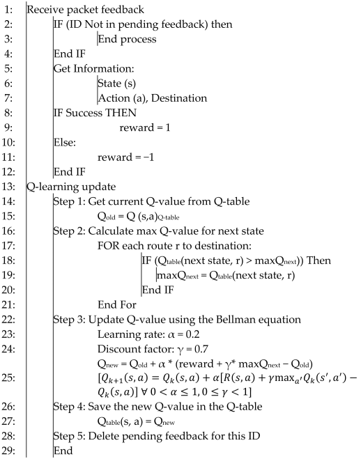
Once this information is received, the algorithm proceeds to update the Q-value Q(s, a) according to the classical Bellman equation that is the foundation of Q-learning. In the equation, the Q-value of the last state-action pair is updated in line with the reward received and estimated future utility. The reward (R) is +1 for successful transmission and −1 for failed transmission, rewarding good routing choices and penalizing poor ones. The update also incorporates the next state’s (s′) maximum Q-value, i.e., maxa′ Q(s′, a′)). This term equals the maximum future reward expected from the next state and is computed by taking into account the same destination D’s current candidate routes. Through this term, the algorithm ensures that not only immediate feedback but also long-term outcomes are considered during learning. Through multiple cycles of feedback and Q-value update, the routing algorithm progressively refines its estimate of which routes perform best under changing network conditions. This iterative learning from feedback allows the AAV network to adapt in real time to mobility, congestion, and other dynamic conditions, ultimately leading to more reliable and efficient route choice. Figure 5 presents the main steps of the proposed procedure for updating the Q value using the Bellman equation, and Algorithm 3 provides the pseudo-code.

Algorithm 3: Update Q value using the Bellman equation

4. Performance Evaluation

4.1. Simulation Setup

To evaluate the performance of the proposed QL-AODV algorithm, we carried out a series of comprehensive simulations using Network Simulator 3 (NS-3.34) [23]. The simulation environment was configured to reflect realistic AAV-network conditions under multiple scenarios.

Table 1. Simulation-environment parameters.

Parameter	Value
Simulator	NS-3.34
Simulation area	800 m × 800 m × 100 m
Simulation time	300 s
Air-interface standard	IEEE 802.11 g
AAV Transmission Range	250 m
Data rate	1024 kbps
Packet size	1024 bytes
Propagation model	Log-distance path loss
Transmission power	18 dBm
Traffic Type	Constant Bit Rate (CBR)
Reception threshold	–85 dBm
AAV velocity	30 m s−1
Simulation runs	20 per configuration

provides the considered simulation parameters, and

Table 2. Q-learning parameters.

Parameter	Value	Description
Learning rate (α)	0.2	Learning rate
Discount factor (γ)	0.7	Discount factor
Initial exploration rate (ε)	0.5	Starting ε
Minimum exploration rate	0.1	εmin
Exploration-decay factor	0.995	εdecay
Maximum routes	10	Upper bound on candidate paths

introduces the considered values of the Q-learning parameters. To evaluate the performance of the proposed QL-AODV, we considered four main performance metrics: packet-delivery ratio (PDR), average throughput, delay and normalized routing load. IEEE 802.11 g is used only as a physical layer proxy in NS-3 simulation, as full 6G cellular air interface specifications are not yet available in simulators. Our QL-AODV protocol operates at the network layer (Layer 3) and is air-interface agnostic, making the routing intelligence directly applicable to 6G cellular infrastructure. This approach of using established air interfaces to validate network-layer protocols for future cellular technologies is standard practice in academic research.

Packet-delivery ratio (PDR) is the percentage of data packets successfully received at all destinations relative to the total number of data packets transmitted from all sources. A higher PDR indicates greater reliability and routing efficiency. PDR can be calculated as follows.

$$\mathrm{PDR}={\displaystyle \frac{\sum \mathrm{Packets} \mathrm{received}}{\sum \mathrm{Packets} \mathrm{sent}}}\times 100\hspace{0.17em}\mathrm{\%},$$

(7)

The average throughput is the total volume of successfully received payload (in kilobits) per unit time (second). It can be calculated as follows.

$$\mathrm{Throughput}={\displaystyle \frac{\sum (\mathrm{Packet} \mathrm{size}\times 8)}{\mathrm{Actual} \mathrm{transmission} \mathrm{time}}}\times {10}^{-3},$$

(8)

Here, the actual transmission time is measured from the moment the first packet is transmitted until the last packet is received; higher throughput signifies more efficient data delivery. For the evaluation process, we considered two main scenarios. In the first scenario, the effect of the change in node density on the performance of the proposed QL-AODV is investigated. The second scenario was introduced to check the impact of the change in node mobility on the performance of the QL-AODV.

Average End-to-End Delay. The average end-to-end delay $\overline{D}$ is defined as the mean time a valid data packet takes to traverse from the source to the destination, including queuing, processing, and transmission delays over all hops. Let $\mathcal{S}$ be the set of data packets successfully received at the destination, and let $t_k^{\mathrm{r}\mathrm{x}}$ and $t_k^{\mathrm{t}\mathrm{x}}$ denote, respectively, the reception and transmission timestamps of packet k. Then

$$\overline{D}\hspace{0.33em}=\hspace{0.33em}{\displaystyle \frac{1}{\left|\mathcal{S}\right|}}\sum _{k\in \mathcal{S}}\left(t_k^{\mathrm{r}\mathrm{x}}-t_k^{\mathrm{t}\mathrm{x}}\right),$$

(9)

Smaller values indicate more stable route selections (avoiding congested nodes), which is consistent with the Q-learning mechanism in QL-AODV that prioritizes states with low buffer occupancy.

Normalized Routing Load (NRL). NRL quantifies the control overhead as the total number of routing control transmissions over the entire network divided by the number of data packets successfully received at their destinations:

$$\mathrm{N}\mathrm{R}\mathrm{L}\hspace{0.33em}=\hspace{0.33em}{\displaystyle \frac{\sum (\mathrm{routing} \mathrm{control} \mathrm{transmissions} \mathrm{over} \mathrm{the} \mathrm{whole} \mathrm{network})}{\sum (\mathrm{data} \mathrm{packets} \mathrm{successfully} \mathrm{received} \mathrm{at} \mathrm{the} \mathrm{destination})}}\times 100\hspace{0.17em}\mathrm{\%}$$

(10)

In the numerator, each time a routing control packet is sent or forwarded by any node counts as one transmission (e.g., RREQ, RREP—including the extended RREP in QL-AODV—RERR, and HELLO if enabled). The denominator counts only successfully delivered data packets. This normalization follows standard practice for comparing ad hoc routing protocols.

4.2. Simulation Results and Discussion

A.

Simulation scenario (I)

In this scenario, we investigated how network density affects routing performance by varying the number of AAV nodes from 15 to 40.

Table 3. Scenario parameters for varying node count.

Parameter	Value
Number of AAV nodes	15, 20, 25, 30, 35, 40
Mobility model	Gauss–Markov
Mean AAV speed	30 m s−1
Simulation time	300 s

provides the specific parameters used during the simulation of this scenario. All AAVs followed the Gauss–Markov mobility model, which offers smooth, moderately predictable trajectories suitable for many AAV applications.

Figure 6 provides the obtained results of the PDR of the proposed QL-AODV compared with the traditional AODV and the hierarchical WBC-AODV [24]. It shows the average PDR at different values of deployed nodes. QL-AODV sustains a markedly higher success rate at every examined density. With 20 nodes, QL-AODV attains a PDR of 94.10%, whereas AODV reaches 85.68% and WBC-AODV yields 87.48%. Even at 40 nodes, QL-AODV still preserves 87.44% compared with 86.12% for AODV and 87.92% for WBC-AODV. This gain stems from QL-AODV’s buffer-aware route selection: as node density rises, congestion probability at intermediate relays increases. AODV, focused chiefly on the shortest-hop metric, may inadvertently traverse overloaded nodes, causing buffer overflows and packet loss. In contrast, QL-AODV incorporates both average and peak buffer occupancy into its Q-learning state, enabling it to learn and prioritize less-congested paths—even if they entail slightly more hops—thereby reducing loss and boosting PDR.

Figure 7 presents the average throughput of the proposed QL-AODV contrasted with AODV and WBC-AODV. QL-AODV likewise delivers higher mean throughput across all densities. For 25 nodes, QL-AODV achieves 983.86 Kbps, versus 962.78 Kbps for AODV and 976.32 Kbps for WBC-AODV. The throughput improvement follows naturally from the superior PDR and the selection of more stable, interruption-resilient routes; by steering clear of congestion hot spots, QL-AODV maintains a smoother data stream. Although all protocols exhibit a modest decline at very high densities (e.g., 40 nodes: QL-AODV 893.05 Kbps vs. AODV 879.71 Kbps vs. WBC-AODV 888.38 Kbps), an expected consequence of heightened channel contention and interference, QL-AODV consistently retains its advantage.

Figure 8 reports the average end-to-end delay as node density increases, showing that QL-AODV consistently achieves the lowest latency by proactively avoiding congested relays. At 20 nodes, QL-AODV records 6.05 ms, compared with 6.27 ms for AODV and 6.90 ms for WBC-AODV; at 40 nodes, QL-AODV maintains 37.37 ms, substantially below 43.43 ms (AODV) and 47.64 ms (WBC-AODV). In mobile ad hoc networks, end-to-end delay is dominated by queueing at intermediate nodes and interruptions due to route maintenance. By encoding both average and peak buffer occupancy into its Q-learning state, QL-AODV learns to select paths with lighter queues and higher route stability—even if they involve slightly more hops—so the reduction in queueing time dominates the small increase in per-hop traversal. This also leads to fewer route errors and rediscovery episodes, eliminating stop-and-go behavior along the flow. In contrast, AODV’s shortest-hop preference tends to traverse overloaded relays, inflating queueing delays, while WBC-AODV’s hierarchical organization curbs discovery flooding but concentrates traffic at cluster heads and may increase hop count, both of which elevate latency. Consequently, QL-AODV delivers consistently lower end-to-end delay than both AODV and WBC-AODV across all examined densities.

Figure 9 summarizes the normalized routing load (NRL). QL-AODV consistently exhibits the lowest overhead among the three protocols. For 20 nodes, QL-AODV attains 4.93%, below 5.14% (AODV) and 5.09% (WBC-AODV). At 35 nodes, QL-AODV records 36.84%, versus 38.93% (AODV) and 39.41% (WBC-AODV). Even at 40 nodes, QL-AODV remains the most efficient with 49.75%, compared to 50.38% (AODV) and 51.22% (WBC-AODV). This reduction is attributable to QL-AODV’s ability to stabilize routes, thereby avoiding frequent route rediscovery (RREQ/RREP) and reducing route error (RERR) events. While WBC-AODV curbs discovery flooding by restricting forwarding to cluster heads and designated relays, its cluster maintenance cost can offset these savings at higher densities; overall, QL-AODV’s learning-driven stability yields the lowest control overhead.

B.

Simulation scenario (II)

In this scenario, we assess the adaptability of QL-AODV to different AAV mobility patterns.

Table 4. Simulation parameters for the varying-mobility scenario.

Parameter	Value
Number of AAV nodes	30
Mean AAV speed	30 m s−1
Simulation time	300 s
Mobility models	Gauss–Markov, Random Direction 2D, Random Walk 2D

provides the specific parameters used during the simulation of this scenario. Three representative mobility models were implemented in NS-3 to gauge the robustness and efficiency of QL-AODV under diverse operating conditions. Each model embodies a distinct level of randomness and predictability, thereby posing different challenges to link maintenance and routing efficiency.

(1)

Gauss–Markov mobility model

This model emulates relatively smooth, predictable flight trajectories, reflecting missions in which AAVs follow pre-planned flight paths. At each time instant, an AAV’s velocity and heading are derived from their previous values plus a small random perturbation, yielding smooth routes that preserve direction and speed over short intervals. It is suited to scenarios where link stability is paramount.

(2)

Random direction 2D mobility model (3D adjusted)

Selected to test protocol behavior when AAVs traverse long legs with fewer abrupt turns than in Random Waypoint. Each AAV chooses a random direction in the horizontal plane and maintains it until reaching a simulation-area boundary, then pauses for 0.1 s before selecting a new direction. The Z-coordinate is adjusted to project the 2D path into three dimensions. This model creates a network with medium volatility.

(3)

Random Walk 2D mobility model (3D adjusted)

The Random Walk model was adopted to examine QL-AODV under the most volatile, unpredictable conditions. Every 0.5 s, each AAV randomly selects a new heading and speed from its current position, yielding highly dynamic, hard-to-predict topologies. The Z-coordinate is likewise adjusted to emulate full 3D movement. Each node is assigned a distinct altitude at initialization, so AAVs operate at different heights throughout the simulation. This model imposes the severest challenge for routing algorithms.

Employing these mobility patterns enables a comprehensive comparison of the proposed QL-AODV with legacy AODV across network conditions ranging from relatively stable to highly unpredictable. Figure 10 and Figure 11 provide the obtained results for this scenario for the three simulated mobility models. The simulation results obtained under diversified mobility models demonstrate that the proposed QL-AODV protocol adapts effectively and delivers markedly higher performance than legacy AODV in every tested scenario. Figure 10 presents the average PDR for the proposed QL-AODV and the traditional AODV for the three simulated mobility models. Furthermore, Figure 11 provides the average throughput for the proposed and traditional AODV models for the three simulated mobility models.

In the relatively stable Gauss–Markov environment, the buffer-aware route-selection mechanism of QL-AODV yields a PDR of 93.41% and an average throughput of 967.74 Kbps. As network volatility increases—from the Random Direction 2-D model to the highly unpredictable Random Walk 2-D model—the learning and fast-adaptation capability of QL-AODV becomes more pronounced: under Random Walk, QL-AODV attains a PDR of 94.86% (approximately a 9.66% relative gain over AODV’s 86.50%) and a throughput about 12.15% higher (974.53 Kbps versus 868.96 Kbps) (Figure 10 and Figure 11, respectively). Figure 12 shows QL-AODV consistently achieves the lowest end-to-end delay across all mobility models, with 16.04 ms under Random Walk compared to 16.44 ms (AODV) and 17.08 ms (WBC-AODV). These improvements arise because QL-AODV continually updates Q-values from live feedback and makes routing decisions that balance hop count with congestion, represented by both average and peak buffer occupancy; consequently, it prioritizes less-congested paths, reduces packet loss, limits route rediscovery and route-error episodes, and maintains smoother traffic flows. While WBC-AODV’s clustering curbs discovery flooding to a certain extent, QL-AODV’s feedback-driven selection achieves lower normalized routing load (e.g., 14.63% versus 18.62% for AODV under Random Walk) and higher delivery efficiency across mobility regimes is shown in Figure 13. Overall, the findings underscore QL-AODV’s suitability for highly dynamic, hard-to-predict AAV networks typical of many real-world missions.

5. Conclusions

The work presents a Q-learning-enhanced AODV (QL-AODV) protocol for AAV networks in 6G settings and revises the evaluation to reflect the added mobility and baseline results. By embedding reinforcement learning into conventional AODV, QL-AODV addresses key limitations of the original protocol in highly dynamic topologies. The design includes an intelligent multipath-collection stage that evaluates up to ten candidate routes and extends the RREP header from 19 to 27 bytes to convey buffer-occupancy information along the path. The Q-state is three-dimensional—normalized hop count, average buffer occupancy, and maximum buffer occupancy—and each source node runs distributed Q-learning with a lightweight exploration–exploitation policy to select routes. NS-3.34 simulations confirm consistent gains. Under the most demanding Random Walk 2-D model, QL-AODV improves PDR by 9.66% (94.86% vs. 86.50% for AODV) and throughput by 12.15% (974.53 Kbps vs. 868.96 Kbps), while also lowering delay (16.04 ms vs. 16.44 ms for AODV and 17.08 ms for WBC-AODV) and NRL (14.63% vs. 18.62% for AODV and 17.62% for WBC-AODV). Across the three mobility regimes (Gauss–Markov, Random Direction, Random Walk), QL-AODV attains higher delivery efficiency and throughput and simultaneously reduces overhead and delay relative to both baselines; across node densities from 15 to 40, it maintains top or near-top PDR and leads in throughput, delay, and NRL. These outcomes arise because QL-AODV learns from live feedback to prioritize less-congested, more stable paths—even when they involve slightly more hops—thereby avoiding overloaded relays, reducing route rediscovery and route-error events, and ultimately enhancing end-to-end service quality.