Parallel and Distributed Frugal Tracking of a Quantile ^†

Abstract

In this paper, we deal with the problem of monitoring network latency. Indeed, latency is a key network metric related to both network performance and quality of service, since it directly impacts on the overall user’s experience. High latency leads to unacceptably slow response times of network services, and may increase network congestion and reduce the throughput, in turn disrupting communications and the user’s experience. A common approach to monitoring network latency takes into account the frequently skewed distribution of latency values, and therefore specific quantiles are monitored, such as the 95th, 98th, and 99th percentiles. We present a comparative analysis of the speed of convergence of the sequential FRUGAL-1U, FRUGAL-2U, and EASYQUANTILE algorithms and the design and analysis of parallel, message-passing-based versions of these algorithms that can be used for monitoring network latency quickly and accurately. Distributed versions are also discussed. Extensive experimental results are provided and discussed as well.

1. Introduction

A key metric for the evaluation of a network service, related to quality of service (QoS) and network performance, is the network latency. Indeed, network latency may disrupt the overall user’s experience: when it is sufficiently high, its impact is devastating since it leads to several problems affecting the user [1,2]. To begin with, the user will experience unacceptably slow response times; moreover, a high network latency usually increases congestion and reduces the throughput, resulting in almost useless communications. From a technical perspective, the  message latency is the time required for a data packet to reach its destination, and it is the sum of several components including transmission, processing, and queuing delay. Latency fluctuations are due to factors such as the distance, the network infrastructure and congestion, the signal propagation, and the time required by network devices to process the data packets in transit. The network latency is measured as the round-trip time taken by a packet from source to destination across the network. It is measured in milliseconds (ms), and its impact on the QoS of a service depends on the specific type of service. For instance, a web server should provide a latency below 100 ms in order to guarantee a responsive browsing experience when the user loads a web page. A higher latency is the source of a perceivable delay that, besides being annoying, may lead to financial losses. In the realm of financial trading, the requirements for latency are stricter and it is not unusual for these kind of services to strive to provide an extremely low latency, measured in microseconds. A trader experiencing a delay during trades may easily decide to switch to a different service. Streaming (video or music) is another fundamental application requiring low latency; currently, a latency below 100 ms can provide a smooth streaming experience. Finally, in order to provide a good experience, voice and video calls require a latency, respectively, below 150 and 200 ms. In practice, the influence of latency on the quality of streaming services depends on the type of streaming: one-way streaming of movies, music, etc., versus multi-way real-time streaming services, such as online gaming or conference calls.

A common approach to monitoring network latency takes into account the frequently skewed distribution of latency values, and therefore specific quantiles are monitored, such as the 95th, 98th, and 99th percentiles [3]. For instance, this is commonly done to precisely assess the latency of a website [4]. In order to meet customer demand and deliver good QoS values, highly requested websites (e.g., a search engine) distribute the incoming traffic load (i.e., the users’ queries) among multiple web server hosts. To compute the overall latency of a website (across all of the associated web server hosts), quantiles must be precisely maintained for each host, and a distributed algorithm is necessary to aggregate individual host responses.

Tracking quantiles on streams is the subject of several studies [5,6,7] and many different algorithms have been devised for this task [8,9,10,11,12,13,14,15,16,17,18,19,20]. Next, we formally define rank and quantile.

Definition 1 

(Rank). Given a multiset S with n elements drawn from a totally ordered universe set $\mathcal{U}$, the rank of the element x, denoted by $R\left(x\right)$, is the number of elements in S less than or equal to x, i.e.,

$$R\left(x\right):=\left|\right\{z\in S\mid z\le x\left\}\right|.$$

(1)

Definition 2 

(q-quantile). Given a multiset S with n elements drawn from a totally ordered universe set $\mathcal{U}$ and a real number $0\le q\le 1$, the inferior q-quantile (respectively, superior q-quantile) is the element $x_q$ whose rank in S is such that

$$x_q\in S:R\left(x_q\right)=\lfloor 1+q·(n-1)\rfloor$$

(2)

(respectively, $R\left(x_q\right)=\lceil 1+q·(n-1)\rceil$).

For instance, $x_0$ and $x_1$ represent, respectively, the minimum and the maximum element of the set S, whilst $x_{0.5}$ represents the median. Frugal [21] is an algorithm for tracking a quantile in a streaming setting; its name reflects the fact that it needs just a tiny amount of memory for this task. Two variants are available, namely Frugal-1U and Frugal-2U; the former uses one unit of memory whilst the latter uses two units of memory in order to track an arbitrary quantile in a streaming setting. EasyQuantile [22] is a recent frugal algorithm designed for the problem of tracking an arbitrary quantile in a streaming setting. This work extends [23] as follows: we shall present a comparative analysis of the speed of convergence of these algorithms; then, we shall design and analyze parallel, message-passing based versions that can be used for monitoring network latency quickly and accurately. Moreover, we shall also discuss the design of their distributed versions. Finally, we shall provide and discuss extensive comparative results.

This paper is organized as follows. Section 2 introduces the sequential Frugal-1U and Frugal-2U algorithms. Section 3 presents the sequential EasyQuantile algorithm. Next, we analyze the speed of convergence of the algorithms in Section 4 and present the design of our parallel, message-passing based versions in Section 5, in which we also discuss corresponding distributed versions. The algorithms are analyzed in Section 6, in which we derive their worst case parallel complexity. Experimental results are presented and discussed in Section 7. Finally, we draw our conclusions in Section 8.

2. The Frugal Algorithm

Among the many algorithms that have been designed for tracking quantiles in a streaming setting, Frugal, besides being fast and accurate, also restricts by design the amount of memory that can be used. It is well known that in the streaming setting, the main goal is to deliver a high-quality approximation of the result (this may provide either an additive or a multiplicative guarantee) by using the lowest possible amount of space. In practice, there is a tradeoff between the amount of space used by an algorithm and the corresponding accuracy that can be achieved. Surprisingly, Frugal-1U only requires one unit of memory to track a quantile. The authors have also designed a variant for the algorithm that uses two units of memory, Frugal-2U. Algorithm 1 provides the pseudo-code for Frugal-1U.

Algorithm 1 Frugal-1U

Require: Data stream S, quantile q, one unit of memory $\tilde{m}$

Ensure: estimated quantile value $\tilde{m}$

$\tilde{m}=0$

for each $s_i\in S$ do

$rand=random(0,1)$

if $s_i>\tilde{m}$ and $rand>1-q$ then

$\tilde{m}=\tilde{m}+1$

else if $s_i<\tilde{m}$ and $rand>q$ then

$\tilde{m}=\tilde{m}-1$

end if

end for

return  $\tilde{m}$

The algorithm works as follows. First, $\tilde{m}$ is initialized to zero, but the authors also suggest to set it to the value of the first incoming stream item in order to accelerate the convergence. This variable will be dynamically updated each time a new item $s_i$ arrives from the input stream S, and its value represents the estimate of the quantile q being tracked. The update is quite simple, since it only requires being increased or decreased by one. Specifically, a random number $0<rand<1$ is generated by using a pseudo-random number generator (the call $random(0,1)$ in the pseudo-code) and if the incoming stream item is greater than the estimate $\tilde{m}$ and $rand>1-q$, then the estimate $\tilde{m}$ is increased, otherwise it is decreased. Obviously, the algorithm is really fast and can process an incoming item in worst-case $O\left(1\right)$ time. Therefore, a stream of length n can be processed in worst-case $O\left(n\right)$ time and $O\left(1\right)$ space.

Despite its simplicity, the algorithm provides good accuracy, as shown by the authors in [21]. However, the proof is challenging since the algorithm’s analysis is quite involved. The complexity in the worst case is $O\left(n\right)$, since n items are processed in worst case $O\left(1\right)$ time.

Finally, the algorithm has been designed to deal with an input stream consisting of integer values distributed over the domain $\left[\mathcal{U}\right]=\{1,2,3,\dots ,\mathcal{U}\}$. This is not a limitation though, owing to the fact that one can process a stream of real values as follows: fix a desired precision, say ${10}^3$, then each incoming stream item with real value can be converted to an integer by multiplying it by ${10}^3$ and then truncating the result by taking the floor. If the maximum number of digits following the decimal point is known in advance, truncation may be avoided altogether: letting m be the maximum number of digits following the decimal point, it suffices to multiply by ${10}^m$. Obviously, the estimated quantile may be converted back to a real number by dividing the result by the fixed precision selected or by ${10}^m$.

Next, we present the Frugal-2U, shown as pseudo-code in Algorithm 2.

This technique is similar to Frugal-1U, but it aims to produce a better quantile estimate utilising just two units of memory for the variables $\tilde{m}$ (the estimate) and $step$, which denotes the update size. It is worth noting that the variable $sign$ can be represented with only one bit and is used to decide whether the estimate should be incremented or decremented.

The $step$ size is dynamically increased or decreased on the basis of the values of the incoming stream items. The update process depends on the function $f\left(x\right)$, and works as follows: if the incoming item falls on the same side of the current estimate, then the variable $step$ is increased; otherwise, it is decreased. To accelerate the convergence, larger update values may be used until the estimate is close to the true quantile value; then, extremely small values are used to increase or decrease $step$.

Algorithm 2 Frugal-2U

Require: Data stream S, quantile q, one unit of memory $\tilde{m}$, one unit of memory $step$, a bit $sign$

Ensure: estimated quantile value $\tilde{m}$

1: $\tilde{m}=0$, $step=1$, $sign=1$

2: for each  $s_i\in S$  do

3:       $rand=random(0,1)$

4:       if $s_i>\tilde{m}$ and $rand>1-q$ then

5:            $step+=(sign>0)?f\left(step\right):-f\left(step\right)$

6:            $\tilde{m}+=(step>0)?\lceil step\rceil :1$

7:            $sign=1$

8:            if $\tilde{m}>s_i$ then

9:                $step+=s_i-\tilde{m}$

10:               $\tilde{m}=s_i$

11:            end if

12:       else if $s_i<\tilde{m}$ and $rand>q$ then

13:            $step+=(sign<0)?f\left(step\right):-f\left(step\right)$

14:            $\tilde{m}-=(step>0)?\lceil step\rceil :1$

15:            $sign=-1$

16:            if $\tilde{m}<s_i$ then

17:               $step+=\tilde{m}-s_i$

18:               $\tilde{m}=s_i$

19:           end if

20:       end if

21:       if $(\tilde{m}-s_i)\ast sign<0\wedge step>1$ then

22:            step = 1

23:       end if

24: end for

25: return  $\tilde{m}$

Of course, there is a tradeoff between speed of convergence and estimation stability. Since this tradeoff is directly related to the $f\left(x\right)$ function, the authors set $f\left(x\right)=1$ to prevent huge oscillations, and we shall use this definition of $f\left(x\right)$ throughout this paper.

Algorithm 2 only updates the estimate when strictly necessary. There are two different scenarios to be considered: the arrival of stream items greater or smaller than the current estimate. Since these two cases are symmetric, we shall just cover the former here. In this particular scenario, an update is required when observing a large stream item. It is worth noting here that the estimation is updated by at least one, and that the $step$ variable is only used when positive. The authors describe this as follows:

“The reason is that when algorithm estimation is close to true quantile, Frugal-2U updates are likely to be triggered by larger and smaller (than estimation) stream items with largely equal chances. Therefore the step is decreased to a small negative value and it serves as a buffer for value bursts (e.g., a short series of very large values) to stabilize estimations. Lines 8–11 are to ensure estimation does not go beyond the empirical value domain when step gets increased to a very large value. At the end of the algorithm, we reset the step if its value is larger than 1 and two consecutive updates are not in the same direction. This is to prevent large estimate oscillations if the step gets accumulated to a large value.”

3. The EasyQuantile Algorithm

This algorithm has been designed to be implemented in the data plane, taking into account stringent constraints on the hardware resources (limited memory and computing capacity). In particular, it works by updating the quantile estimate $\tilde{m}$ depending on the actual count of the stream items; updates are performed only if required, i.e., if the estimate deviates from the true quantile. A key idea is to distinguish between smaller and larger quantiles using an experimentally determined toggling threshold $toggleThreshold$, fixed by the authors at 0.7. For small quantiles, the update is smooth, being based on the average of the observed stream items, whilst for large quantiles, the update is more drastic, being based on the current range (max value minus min value).

The algorithm begins initializing the variables used internally, then proceeds determining the mode of operation, which can be either $MAX\_MIN$ if the quantile to be tracked is greater than the toggling threshold or $AVERAGE$ otherwise. Next, the incoming stream items are processed. The arrival of a new item $s_i$ increases the value of $count$, which keeps track of the number of observations seen. Only for the first observed item, the quantile estimate $\tilde{m}$ is set to 1 and the algorithm proceeds waiting for the next incoming item. Otherwise, for each successive item, the algorithm computes $threshold$, a dynamically adjusting threshold given by the product $count\times quantile$. Next, the algorithm dynamically adjusts the current values of $max$ and $min$ and the current value of $sum$, which is the sum of the values of the observations seen so far.

The step of the update is then computed, depending on the mode of operation. The algorithm then selectively updates the quantile estimate depending on the values of $countLow$ and $countHigh$. Those variables are initialized to zero and represent, respectively, the number of items whose value is lesser or greater than the current quantile estimate $\tilde{m}$. This allows avoiding sorting to infer the rank of the estimate. If the incoming item $s_i$ is less than or equal to the quantile estimate $\tilde{m}$, the value of $countLow$ must be increased by one, otherwise the value of $countHigh$ must be increased by one. Here, the authors take advantage of the fact that, after seeing the i-th item, the values of $countLow$ and $countHigh$ must be respectively equal to $i\times q$ and $i\times (1-q)$ if $\tilde{m}$ is equal to the true quantile value. Therefore, if $countLow+1$ exceeds the dynamically adjusted $threshold$ value, the current estimate $\tilde{m}$ is greater than the true quantile, and the algorithms updates the estimate by subtracting the previously computed step size $\lambda$. The reason behind the increase in $countHigh$ is that, immediately after the update, the estimate is less than its previous value and the authors treat the estimate as if it was an incoming stream item. The other update is symmetric for the case $s_i>\tilde{m}$: if $countHigh+1$ exceeds $count-threshold$ (i.e., $i\times (1-q)$), following the previous argument, the authors update the estimate by adding $\lambda$ and increasing $countLow$, again treating the estimate as a stream item.

Algorithm 3 provides the pseudo-code for EasyQuantile.

Algorithm 3 EasyQuantile

Require: Data stream S, quantile q, $O\left(1\right)$ units of memory

Ensure: estimated quantile value $\tilde{m}$

$mode=0$                                        ▹ mode of operation: $MAX\_MIN=1,AVERAGE=2$

$\tilde{m}=0$

$max=-\infty$

$min=+\infty$

$sum=0$

$count=0$

$countLow=0$

$countHigh=0$

$\lambda =0$

$count=0$

$threshold=0$

$toggleThreshold=0.7$

if $q>toggleThreshold$  then

$mode=1$

else

$mode=2$

end if

for each $s_i\in S$  do

$count=count+1$

if $count\le 1$ then

$\tilde{m}=s_i$

continue                                                                             ▹ go to the next iteration

end if

$threshold=count\times quantile$

if $s_i<min$ then

$min=s_i$

end if

if $s_i>max$ then

$max=s_i$

end if

$sum=sum+s_i$

if $mode==1$ then

$\lambda ={\displaystyle \frac{max-min}{count}}$

else

$\lambda ={\displaystyle \frac{sum}{count\times (count-1.0)}}\times 2.0$

end if

if $s_i\le \tilde{m}$ then

if $countLow+1>threshold$ then

$\tilde{m}=\tilde{m}-\lambda$

$countHigh=countHigh+1$

else

$countLow=countLow+1$

end if

else

if $countHigh+1>count-threshold$ then

$\tilde{m}=\tilde{m}+\lambda$

$countLow=countLow+1$

else

$countHigh=countHigh+1$

end if

end if

end for

return $\tilde{m}$

4. Speed of Convergence

We experimentally determined the speed of convergence to the true quantile of Frugal-1U, Frugal-2U, and EasyQuantile by implementing the sequential versions of the algorithms and keeping track of pairs $(\widetilde{m_i},q_i),i=n/100,2n/100,\cdots ,99n/100,n$ (i.e., each pair is computed every 1/100 of the input stream, whose length is n). We carried out our experiments using the synthetic datasets shown in

Table 1. Synthetic datasets.

Dataset	Distribution	Parameters	PDF
D1	Uniform	[0, 25,000]
D2	${\chi }^2$	$\alpha =5$
D3	Exponential	$\alpha =0.5$
D4	Log-normal	$\alpha =1,\beta =1.5$
D5	Normal	$\mu =50,\sigma =2$
D6	Cauchy	$\alpha$ = 10,000, $\beta$ = 1250
D7	Extreme Value	$\alpha =20,\beta =2$
D8	Gamma	$a=2,b=4$

.

In particular, we performed three sets of experiments. First, we assessed the speed of convergence by fixing the quantile to be tracked to 0.99 and the dataset size to 10 millions, and varying the distribution. Next, we fixed the distribution (to the normal distribution), fixed the quantile to be tracked (to 0.99), and varied the stream size. Finally, we fixed the distribution (to the normal distribution), fixed the dataset size (to 10 millions), and varied the quantile to be tracked.

Figure 1 and Figure 2 depict the results obtained varying the distribution.

As shown in Figure 1a, related to the normal distribution, all of the algorithms require slightly more than 4 million items before converging initially to the true quantile at that moment, which then slowly rises. The algorithms track the quantile and reach again the true quantile at about 9 million items, then the algorithms closely follow the true quantile evolution until the end of the stream.

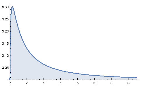
The behavior depicted for the cauchy distribution in Figure 1b markedly differs between the Frugal-1U and Frugal-2U algorithms on the one side, and EasyQuantile on the other. The former closely follow the true quantile up to about 9 million items. The true quantile then rapidly increases and is reached again just at the end of the stream. The EasyQuantile algorithm consistently exhibits problems in tracking the quantile, even though sudden jumps present in the plot show that the algorithm periodically converges but then has difficulties until about 8 million items. At that moment, the true quantile begins to drift and the algorithm slowly chases it until convergence at the end of the stream.

The uniform distribution, shown in Figure 1c, is characterized by an almost regular and linear behavior exhibited by all of the algorithms with regard to the tracking of the true quantile. Frugal-1U is the slowest, followed by Frugal-2U. Starting from about 1.5 million items, EasyQuantile is consistently faster than the others, even though both Frugal-1U and Frugal-2U converge to the true quantile at the end of the stream.

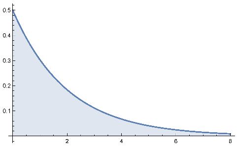
Figure 1d is related to the exponential distribution. The behavior of EasyQuantile, starting at about 1 million items, appears to be close to linear and a final sudden jump allows the algorithm to converge to the true quantile. Both Frugal-1U and Frugal-2U exhibit the same behavior and are able to converge 4 times to the true quantile value before finally converging at the end of the stream.

Regarding the ${\chi }^2$ distribution, depicted in Figure 2a, the behavior of the algorithms is pretty similar to that observed for the exponential distribution, with the EasyQuantile algorithms exhibiting an almost linear trend starting from about 3 million items. Frugal-1U and Frugal-2U, after initially converging at about 6 million items, converge again at about 8.5 million items and then continue to closely track the true quantile value until the end of the stream.

The algorithms’ behaviors for the gamma distribution, shown in Figure 2a, are also quite similar to that for the ${\chi }^2$ and exponential distributions, which is not surprising owing to the relationships between the ${\chi }^2$, gamma, and exponential distributions.

In the case of the log-normal distribution, shown in Figure 2c, all of the algorithms closely track the true quantile until about 5.5 million items. Here, the true quantile value starts drifting. EasyQuantile slowly approaches it with a linear behavior and a sudden jump at the end, whilst Frugal-1U and Frugal-2U are faster in adapting, reach again the true quantile at about 8.5 million items and then closely chase it until the end of the stream.

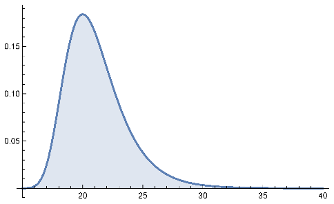
The extreme value distribution is depicted in Figure 2d. As shown, all of the algorithms exhibit a linear trend. However, Frugal-1U and Frugal-2U, starting from about 7.5 million items, modify their behavior and adapt faster than EasyQuantile, better tracking the true quantile until the end of the stream, where, with a sudden jump, EasyQuantile is also able to converge.

Next, we analyze the convergence speed when varying the stream size. Results are reported in Figure 3. As shown, we used stream sizes equal to 1, 10, 50, and 100 million items. Note that Figure 3b is a copy of Figure 1a, but is reported here for completeness. Figure 3a is more interesting than the others (which are quite similar with regard to their behavior, already discussed with reference to Figure 1a) since it shows that the Frugal-1U estimate goes down up to 200 thousand items instead of being incremented, and the same behavior is also observed for Frugal-2U (up to about 150 thousand items).

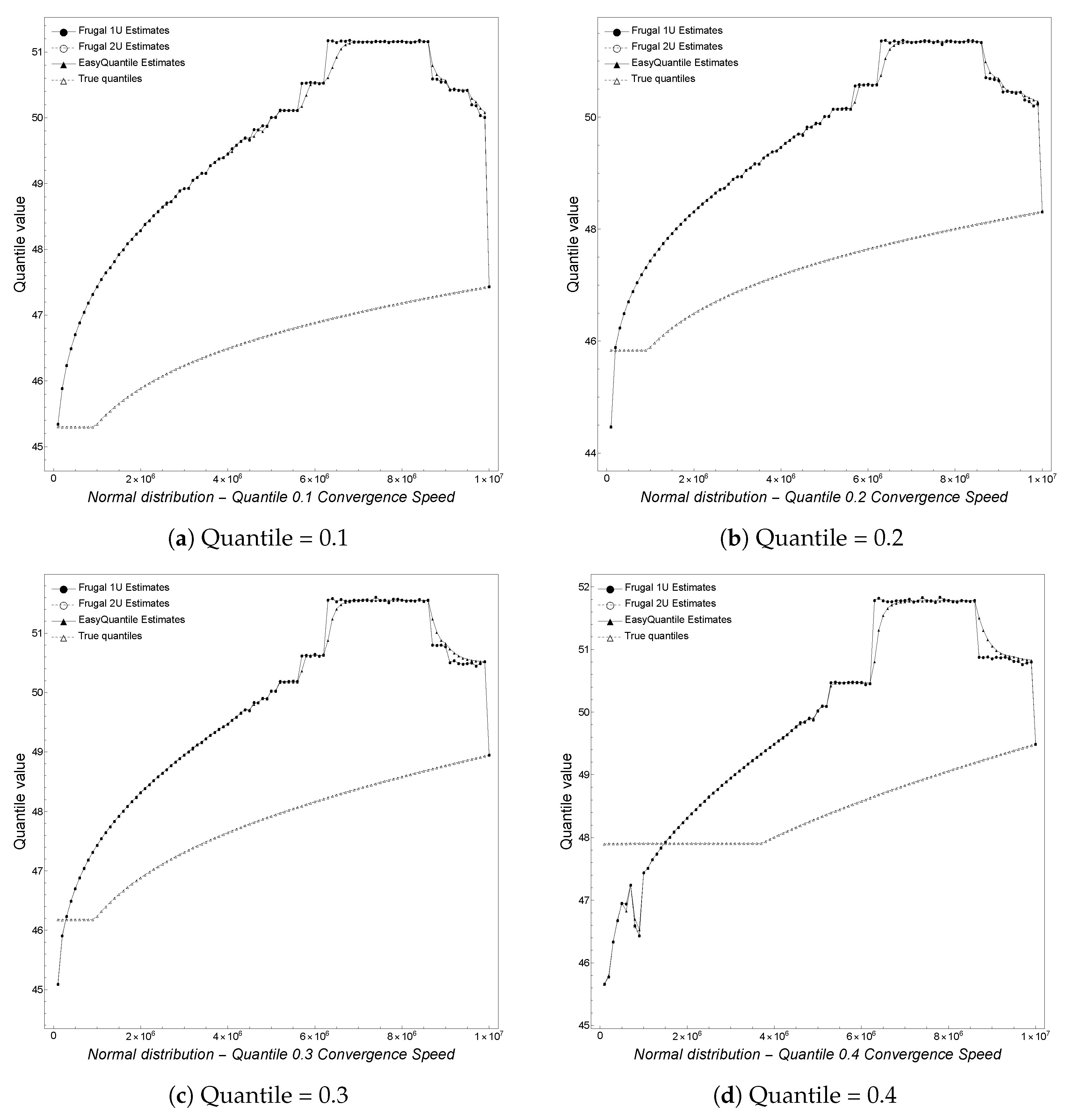
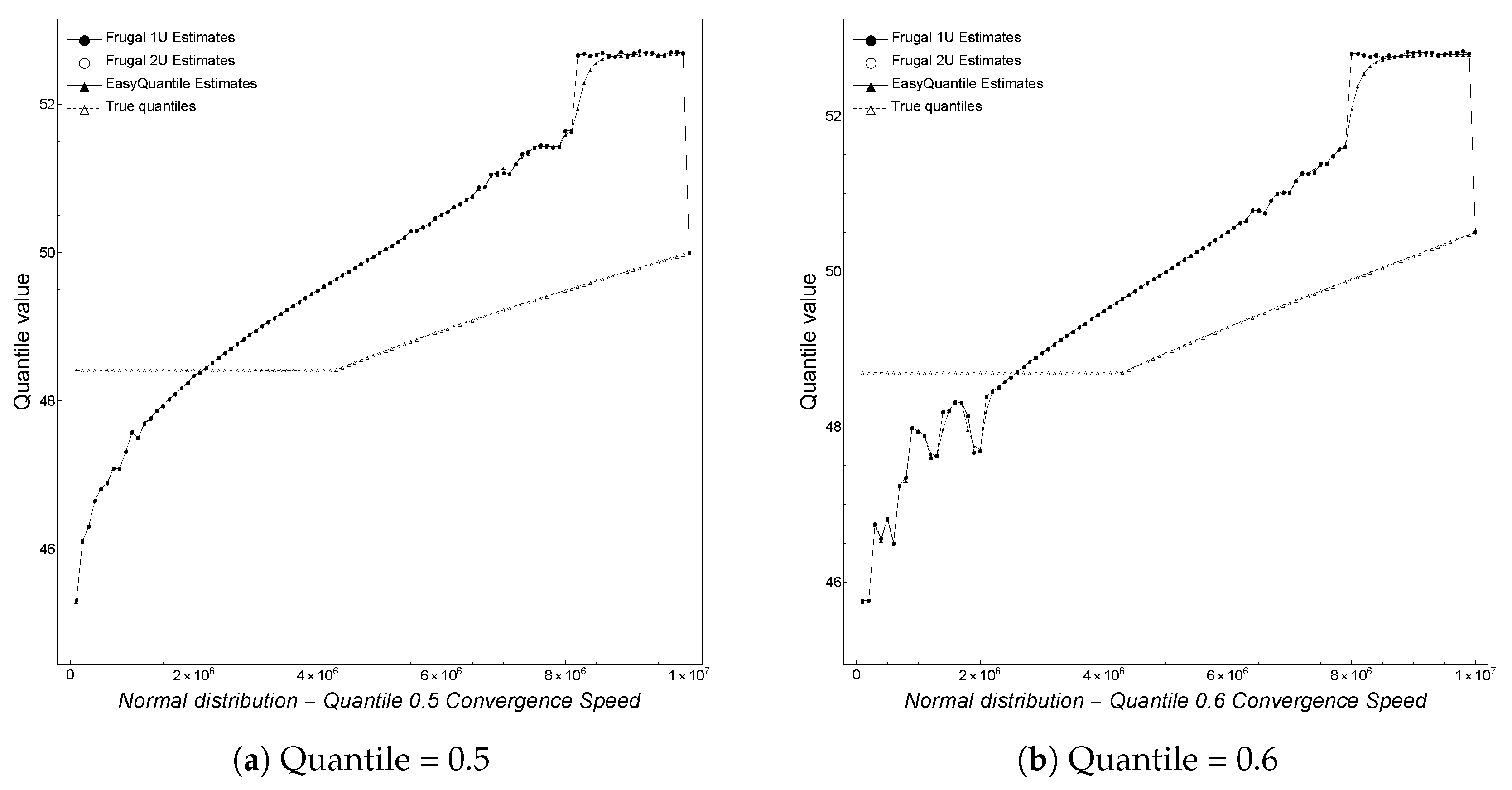
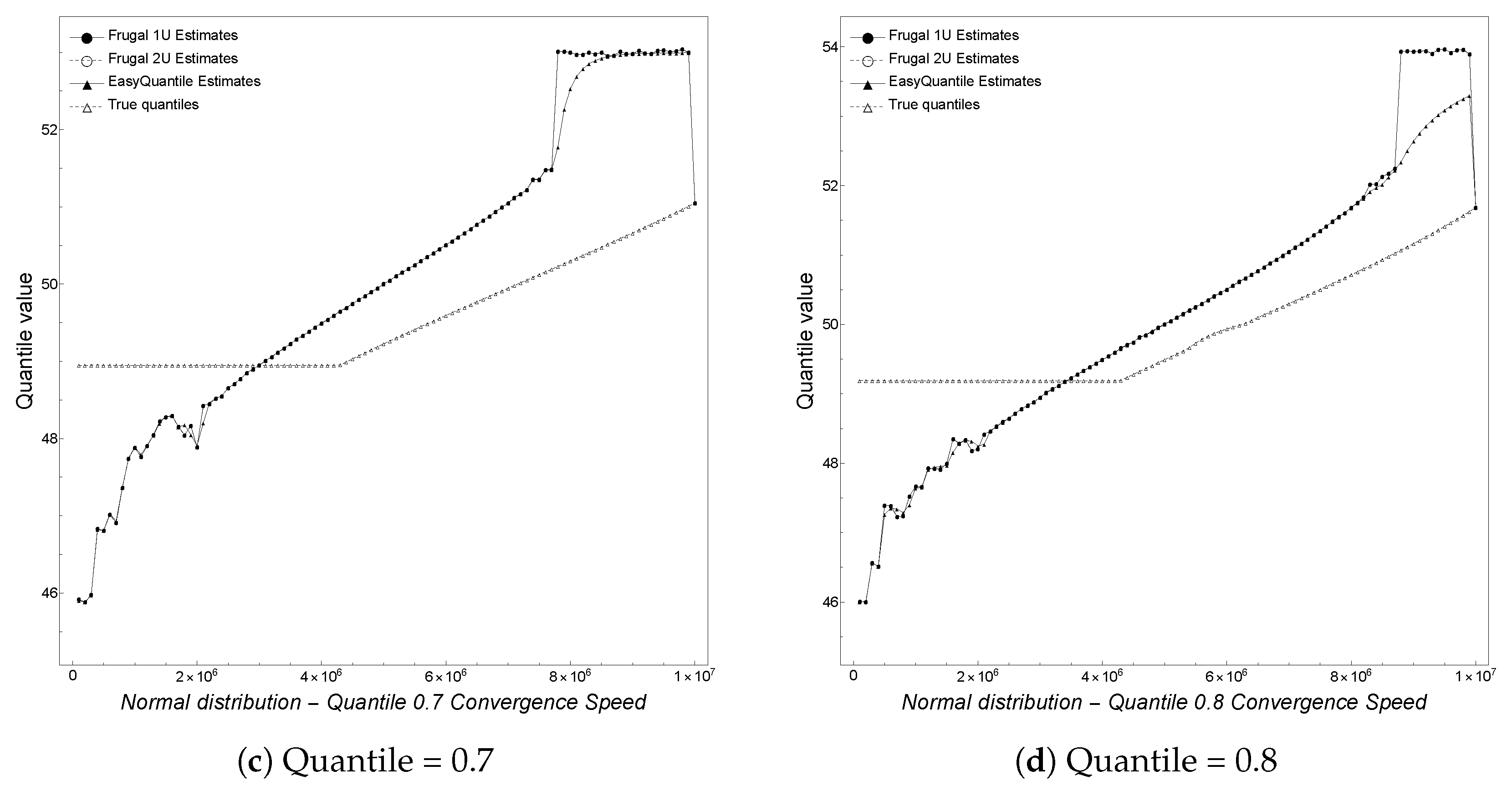
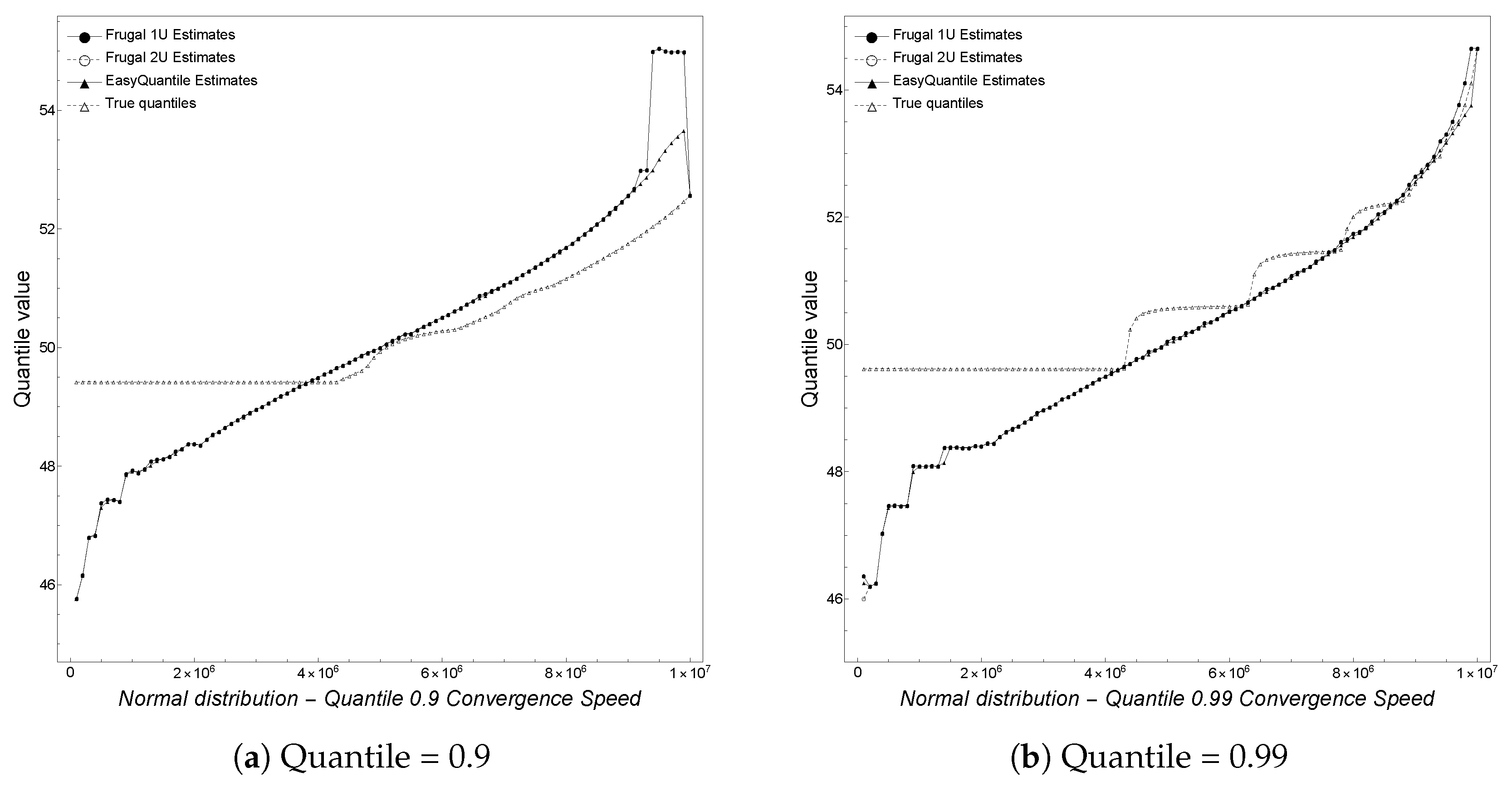
Finally, we analyze the convergence speed with regard to the actual quantile being tracked. In particular, we track equi-spaced quantiles $0.1,0.2,\cdots ,0.8,0.9$, and 0.99. We note here that the plot for the 0.99 quantile is a copy of Figure 1a but is reported here for completeness. As shown in Figure 4, Figure 5 and Figure 6, depicting the results obtained by varying the quantile, we observe that for smaller quantiles (0.1, 0.2, and 0.3), all of the algorithms overestimate the true quantile value until convergence at the end of the stream. This behavior changes starting from the 0.4 quantile on, with an underestimation phase followed by an overestimation one. Overall, the algorithms are better at tracking higher rather than smaller quantiles.

5. Parallelizing the Frugal Algorithm

In this section, we design parallel, message-passing based versions of algorithms. Since the parallel design is the same for all of the algorithms, we shall illustrate these with reference only to Frugal-1U. A corresponding distributed version (this also applies to all of the algorithms) can be easily derived from the parallel one and shall be discussed along with the parallel one. In order to parallelize Frugal-1U, we begin by partitioning the input among the available processors.

For the parallel version, we assume that the input consists of a dataset S of size n. Therefore, assuming that p processors are available, the input is partitioned so that each processor is responsible for either $\lfloor n/p\rfloor$ or $\lceil n/p\rceil$ items.

For the distributed version, each processor will instead process a sub-stream $S_i$ of length $n_i$, $i=1,\cdots ,p$. Each processor will update locally its own estimate of the quantile q being sought.

After processing its input, the processors in the parallel version will engage in a parallel reduction operation, required to aggregate the local estimates obtained. Similarly, in the distributed version, the processors will send their local information to a designated processor, which will take care of performing the required aggregation step to obtain the global estimate associated to the union of the sub-streams ${\cup }_{i=1}^p{S}_i$.

The information required for the final aggregation operation is the same for both the parallel and the distributed version, namely for each processor $i=1,\cdots ,p$, we need a pair $({\tilde{m}}_i,n_i)$, where ${\tilde{m}}_i$ and $n_i$ are, respectively, the local estimate and the number of items processed by the i-th processor.

The local results obtained by the processors are aggregated in parallel by performing a reduction operation in which the weighted average of the local estimates is computed using the $n_i$ as weights. Note that ${\sum }_{i=1}^p{n}_i=n$. Letting ${\tilde{m}}_g$ denote the global estimate for the input dataset S (parallel case) or the union ${\cup }_{i=1}^p{S}_i$ (distributed case), it holds that

$${\tilde{m}}_g={\displaystyle \frac{{\sum }_{i=1}^p{\tilde{m}}_i{n}_i}{n}}.$$

(3)

Algorithms 4 and 5 provide, respectively, the pseudo-code for the parallel version of Frugal-1U and the user’s defined parallel reduction operator in charge of computing the global estimate. In Algorithm 4, we assume that the input is a dataset D of size n stored into an array A. The input parameters are, respectively, A, n, p, and q, where A is the input array, n the length of A, p the number of processors we use in parallel and q the quantile to be estimated.

Algorithm 4 Parallel Frugal-1U

Require: A, an array; n, the length of A; p, the number of processors; q, the quantile to be estimated

Ensure: estimated quantile value $\tilde{m}$

// let $id$ be the rank of the processor $(0\le id\le p-1)$

$left=\lfloor idn/p\rfloor$

$right=\lfloor (id+1)n/p\rfloor -1$

${\tilde{m}}_{id}=$ Frugal-1U$(A,left,right,q)$

$siz{e}_{id}=right-left+1$

$({\tilde{m}}_g,w_g)=$ ParallelReduction$({\tilde{m}}_{id},siz{e}_{id})$

if  $id==0$  then

return ${\tilde{m}}_g$

end if

The algorithm begins by partitioning the input array; $left$ and $right$ are, respectively, the indices of the first and last element of the array assigned to the process with rank $id$ by the domain decomposition performed. This is done by using a simple block distribution. We assume that each process receives as input the whole array A, for instance, every process reads the input from a file or a designated process reads it and broadcasts it to the other processes. Therefore, there is no need to use message–passing to perform the initial domain decomposition.

Next, the algorithm locally estimates the quantile q for its sub-array. The modification required to the sequential Frugal-1U is trivial, and consists of coding a linear scan of the sub-array using a for loop starting at $left$ and ending at $right$.

Once the local estimates ${\tilde{m}}_{id}$, $id=0,\cdots p-1$ have been found, the processors engage in a parallel reduction operation by invoking the ParallelReduction algorithm passing as input the pair $({\tilde{m}}_{id},siz{e}_{id})$. Its purpose is to determine the global estimate of the quantile q for the whole array A, and this is done by using the parallel reduction operator of Algorithm 5. The parallel reduction can be either a standard user’s defined parallel reduction in which only one of the processors obtains the result at the end of the computation or it may be an all-reduction, which differs because in this case all of the processors obtain the result at the end of the computation. In practice, an all-reduction is equivalent to a reduction followed by a broadcast operation. Here, we choose a standard reduction in which we assume that the processor with rank equal to zero will obtain the final result but, in this case, it is trivial to use an all-reduction if required.

As shown in Algorithm 5, the parallel reduction takes as input two pairs $({\tilde{m}}_i,n_i)$ and $({\tilde{m}}_j,n_j)$ produced by processors i and j and returns the pair $(\tilde{m},w)$, where $w=n_i+n_j$ and $\tilde{m}=({\tilde{m}}_i{n}_i+{\tilde{m}}_j{n}_j)/w$.

Algorithm 5 Parallel reduction operator

Require: pairs $({\tilde{m}}_i,n_i)$ and $({\tilde{m}}_j,n_j)$ produced by processors i and j

Ensure: estimated quantile value $\tilde{m}$, weight w

$w=n_i+n_j$;

$\tilde{m}=({\tilde{m}}_i{n}_i+{\tilde{m}}_j{n}_j)/w$

return  $(\tilde{m},w)$

The corresponding parallel versions for Frugal-2U and EasyQuantile are obtained by substituting these algorithms in place of the invocation of Frugal-1U in Algorithm 4, since Algorithm 5 is the same for all of the algorithms. Similar considerations can be used to derive the distributed versions. It is worth noting here that, from a practical perspective, the only differences between a parallel algorithm and a distributed one are the following: (i) the distributed nodes’ hardware may be heterogeneous, whilst a parallel machine is typically equipped with identical processors; (ii) the network connecting the distributed nodes is typically characterized by relatively high latency and low bandwidth, whilst, on the contrary, the interconnection network of a parallel machine provides ultra low latency and high bidirectional bandwidth; (iii) some of the distributed nodes may fail in unpredictable ways whilst we expect the nodes of a parallel machine to be always up and running (except for scheduled maintenance). As a consequence, only the performance may be affected whilst the accuracy is identical. Here, we are assuming that the distributed nodes stay up and running during the distributed computation.

6. Analysis of the Algorithm

Here, we derive the parallel complexity of the algorithm (the analysis applies to Frugal-2U and EasyQuantile as well). At the beginning, the workload is balanced using a block distribution; this is done with two simple assignments; therefore, the complexity of the initial domain decomposition is O(1). Determining a local estimate ${\tilde{m}}_{id}$ invoking the Frugal-1U algorithm requires in the worst case $O(n/p)$ time, since the running time of the sequential algorithm is linear and the sub-array to be processed consists of either $\lfloor n/p\rfloor$ or $\lceil n/p\rceil$ items. Determining the weight $siz{e}_{id}$ requires worst case $O\left(1\right)$ time.

The parallel reduction operator is used internally by the ParallelReduction step. Since this function is called in each step of the ParallelReduction and its complexity is $O\left(1\right)$, the overall complexity of the ParallelReduction step is $O(logp)$ (using, for instance, a binomial tree [14] or even a simpler binary tree). Therefore, the overall parallel complexity of the algorithm is $O(n/p+logp)$. We are now in the position to state the following theorem:

Theorem 1. 

The algorithm is cost-optimal.

Proof. 

Cost-optimality [24] requires by definition that asymptotically $p{T}_p=T_1$, where $T_1$ represents the time spent on one processor (sequential time) and $T_p$ is the time spent on p processors. The sequential algorithm requires $O\left(n\right)$, and the parallel complexity of the algorithm is $O(n/p+logp)$. It follows from the definition that the algorithm is cost-optimal for $n=\Omega (plogp)$. □

We proceed with the analysis of iso-efficiency and scalability. The sequential algorithm has complexity $O\left(n\right)$; the parallel overhead is $T_o=p{T}_p-T_1$. In our case, $T_o=p(n/p+logp)-n=plogp$. The iso-efficiency relation [25] is then $n\ge plogp$. Finally, we derive the scalability function of this parallel system [26].

This function shows how memory usage per processor must grow to maintain efficiency at a desired level. If the iso-efficiency relation is $n\ge f\left(p\right)$ and $M\left(n\right)$ denotes the amount of memory required for a problem of size n, then $M\left(f\right(p\left)\right)/p$ shows how memory usage per processor must increase to maintain the same level of efficiency. Indeed, in order to maintain efficiency when increasing p, we must increase n as well, but on parallel computers, the maximum problem size is limited by the available memory, which is linear in p. Therefore, when the scalability function $M\left(f\right(p\left)\right)/p$ is a constant C, the parallel algorithm is perfectly scalable; $Cp$ represents instead the limit for scalable algorithms. Beyond this point, an algorithm is not scalable (from this point of view).

In our case, the function describing how much memory is used for a problem of size n is given by $M\left(n\right)=n$. Therefore, $M\left(f\right(p\left)\right)/p=O\left(\log p\right)$ with $f\left(p\right)$ given by the iso-efficiency relation and the algorithm is moderately scalable (again, from this perspective, related to the amount of memory required per processor).

7. Experimental Results

In this section, we present and discuss the results of the experiments carried out for the parallel versions of Frugal-1U, Frugal-2U, and EasyQuantile, showing that the parallel versions of these algorithms are scalable and the parallelization does not affect the accuracy of the quantile estimates with respect to the estimate done with the sequential versions of the algorithms.

The tests have been carried out on both a parallel machine and a workstation. The former is the Juno supercomputer (peak performance 1.134 petaflops, 12,240 total cores, 512 GB of memory per node, Intel OmniPath 100 Gbps interconnection, lustre parallel filesystem) kindly made available by CMCC. Each node is equipped with two 2.4 GHz Intel Xeon Platinum 8360Y processors, with 36 cores each, and some nodes are also equipped with two NVIDIA A100 GPUs. The source code has been compiled using the Intel C++ compiler and the Intel MPI library.

The workstation is a HP (Hewlett-Packard) machine equipped with a 24 core Intel XEON W7-2495X processor and 256 GB of memory, and two NVIDIA RTX 4090 GPUs.

The tests have been performed on the synthetic datasets reported on Table 1. The experiments have been executed, varying the distribution, number of cores, stream length, and the quantile being tracked.

Table 2. Default settings of the parameters.

Parameter	Values
quantiles	$\{0.1,0.2,0.3,0.4,0.5,0.6,0.7,0.8,0.9,0.95,0.99\}$
number of cores P	$\{36,72,144,288\}$
stream length	$\{25.6B$ (strong scaling), $45M$ (weak scaling) }

reports the default settings for the parameters used on the parallel machine. On the workstation, the number of cores was 2, 4, 8, and 16 whilst the stream length was 100 millions for strong scalability and 100 millions per core for weak scalability.

7.1. Parallel Machine

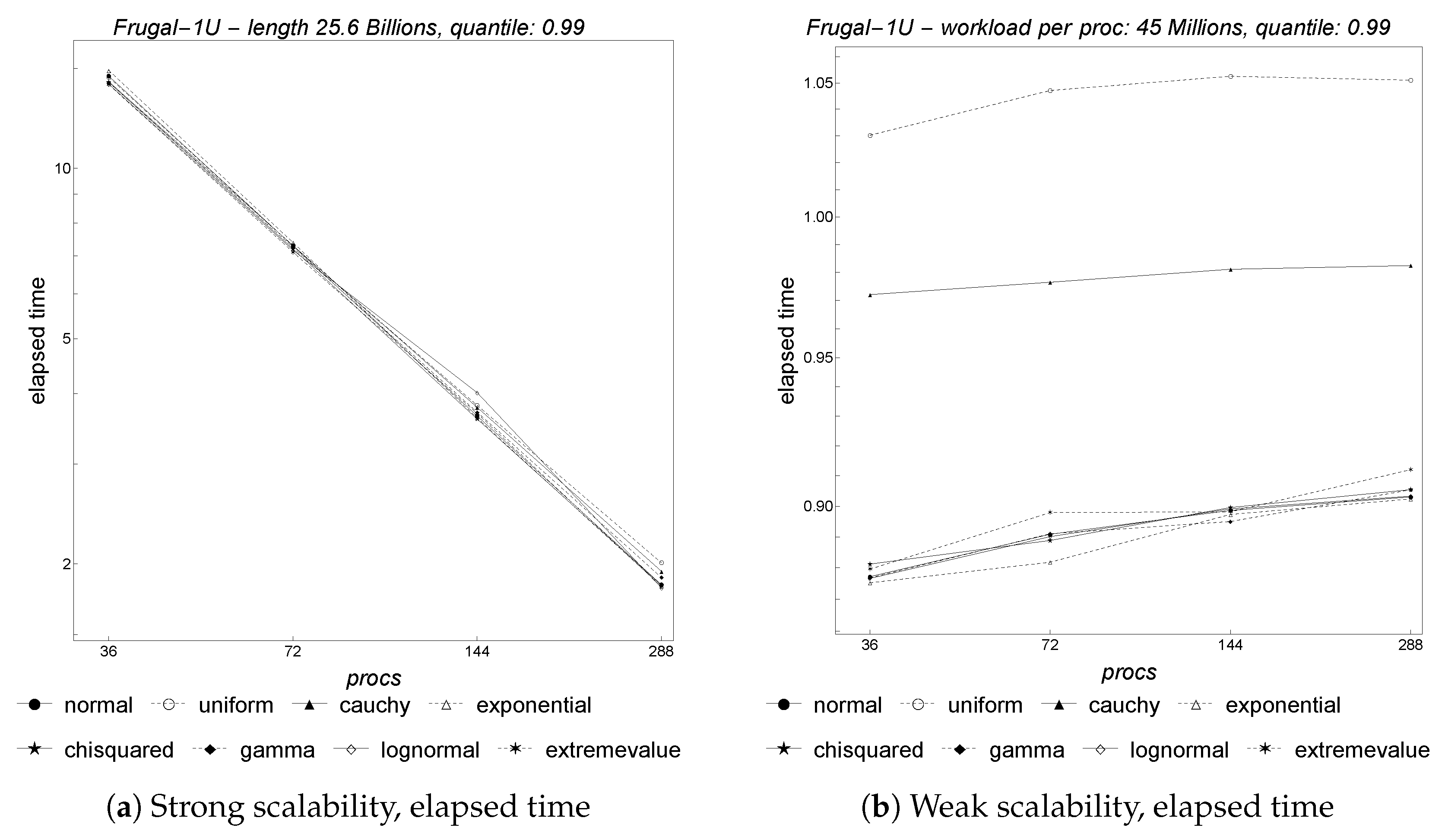
We begin by providing the results obtained for each algorithm when considered in isolation. Figure 7 depicts the results for parallel Frugal-1U with regard to both strong and weak scalability. To analyze the strong scalability, we set the length of the input stream to 25.6 billion items, track the 0.99 quantile, and vary the number of cores and the distributions. Figure 7a shows the results using a log–log plot of the parallel runtime versus the number of cores. A straight line with slope $-1$ indicates good scalability, whereas any upward curvature away from that line indicates limited scalability. As shown, parallel Frugal-1U exhibits overall strong scaling almost independently from the underlying input distribution being used.

Next, we discuss the weak scalability. In this case, the problem size increases at the same rate as the number of processors, with a fixed amount of work per processor. A horizontal straight line indicates good scalability, whereas any upward trend of that line indicates limited scalability. In Figure 7b, the amount of work per core is fixed at 45 million items and we track the 0.99 quantile. Almost all of the distributions considered exhibit good weak scalability starting from 72 cores.

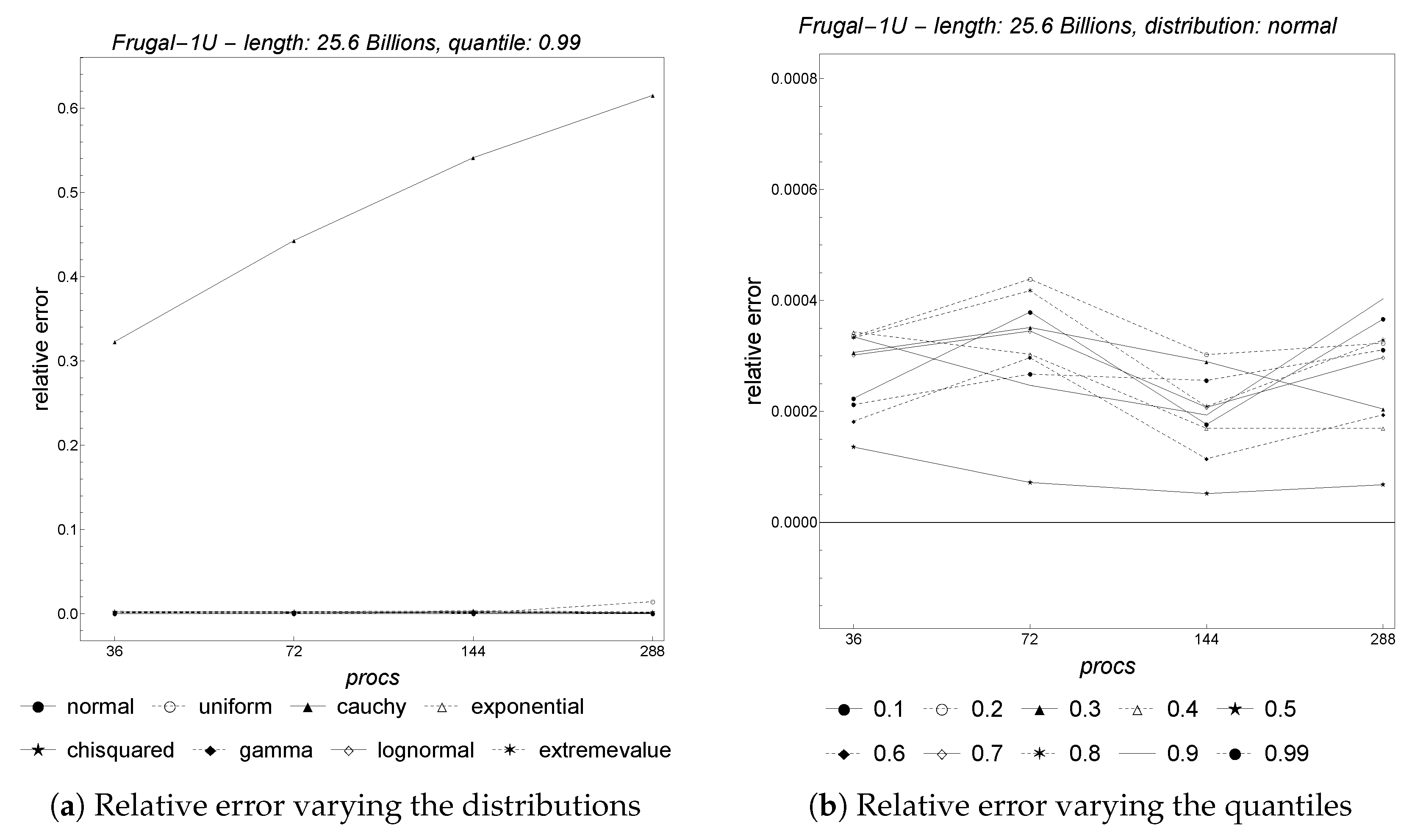
Figure 8 provides the results obtained for the accuracy, measured using the relative error between the true and the estimated quantile value. We perform the test for both distributions (Figure 8a) and quantiles (Figure 8b). As shown, the cauchy distribution confirms its adversarial character for the algorithm, with a relative error steadily rising from slightly more than 0.3 on 36 cores to about 0.6 on 288 cores. The other distributions do not impact the relative error, which is almost zero. This holds true also for the uniform distribution, whose relative error steadily rises from about ${10}^{-5}$ on 36 cores to about ${10}^{-2}$ on 288 cores.

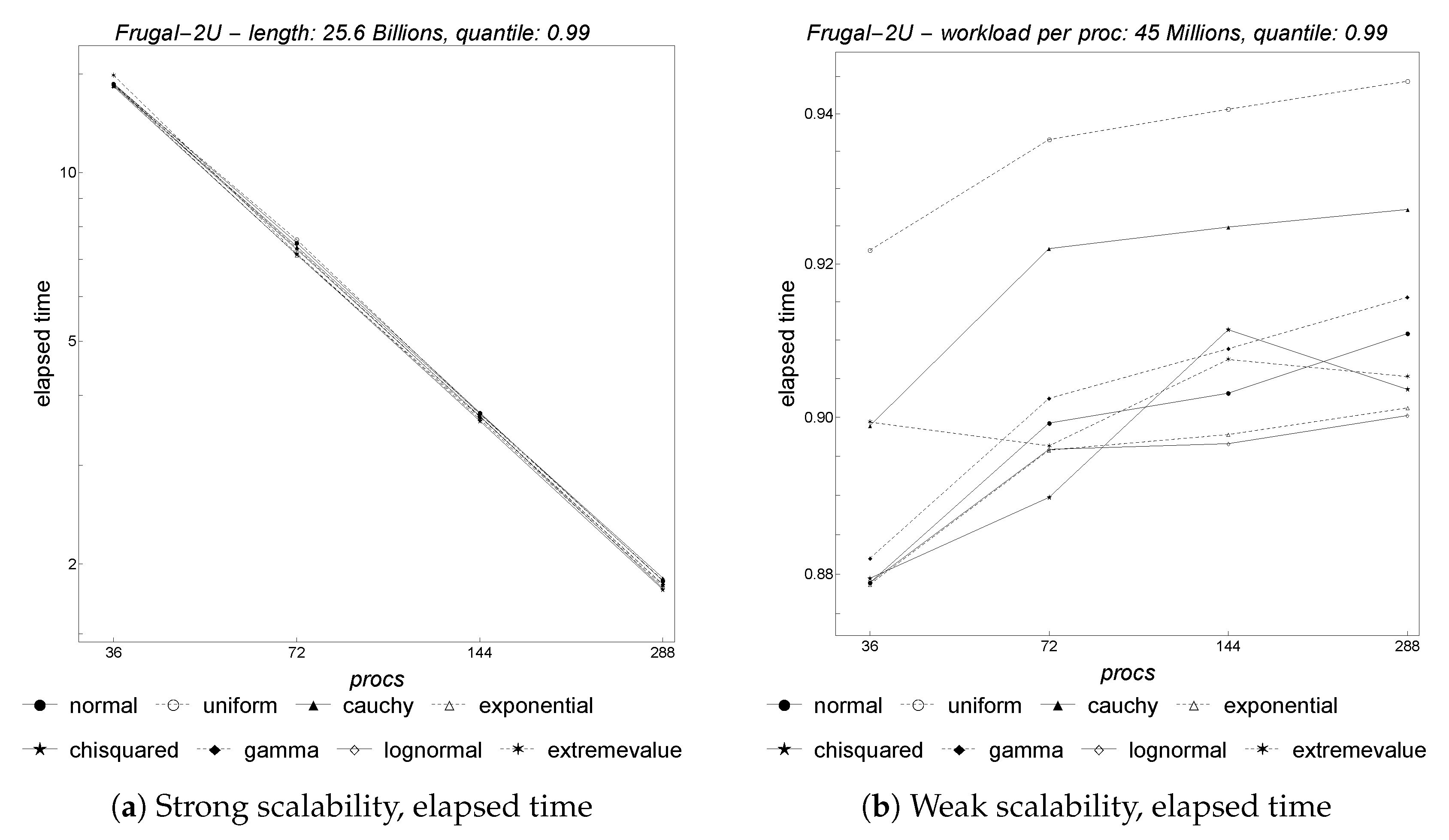
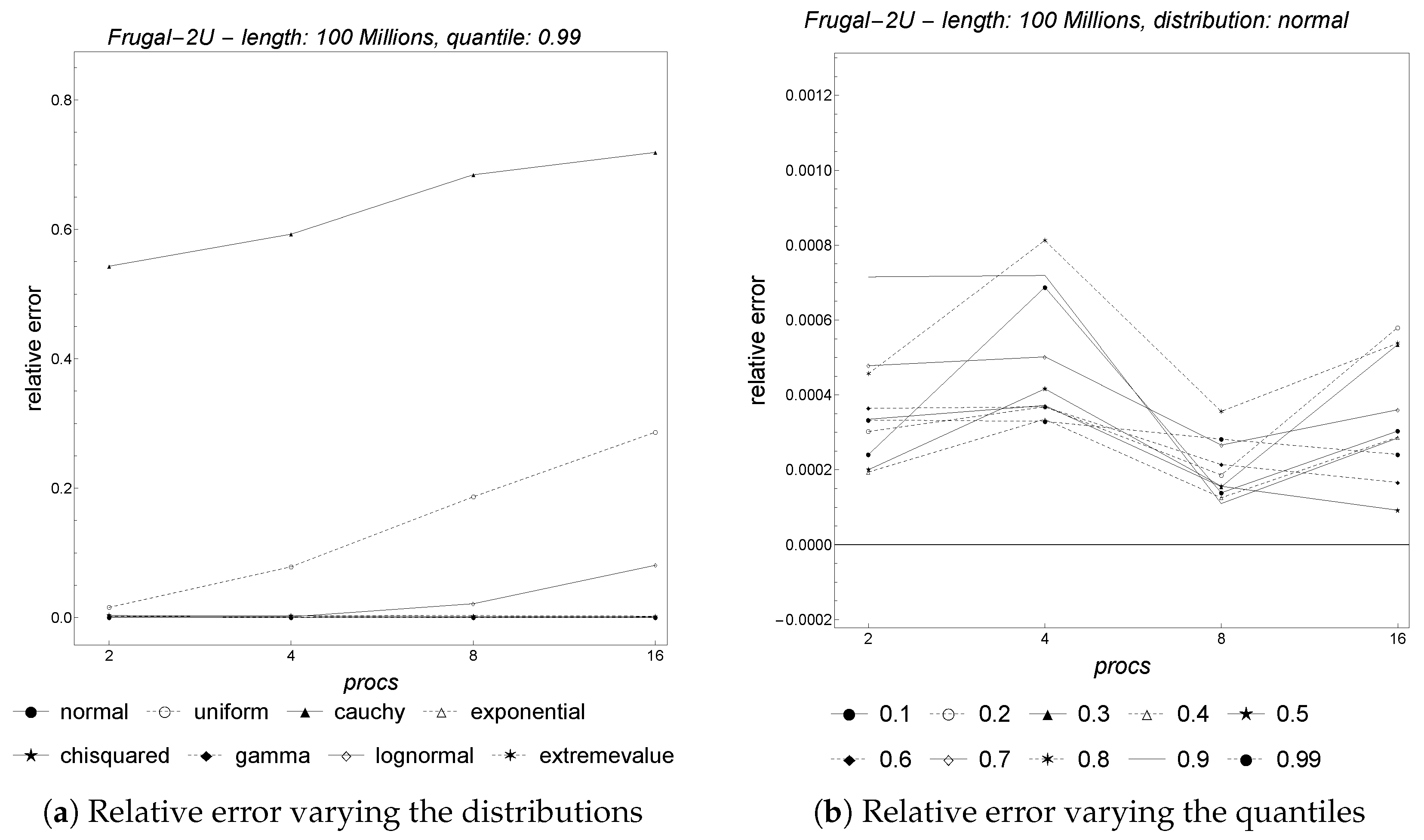
Figure 9 depicts the results for parallel Frugal-2U with regard to both strong and weak scalability. As shown, the behavior of this algorithm is substantially equal to that of Frugal-1U with regard to strong scaling. However, weak scalability is consistently worse. The behavior, with regard to accuracy, shown in Figure 10, is again quite similar to that of Frugal-1U.

Figure 11 depicts the results for parallel EasyQuantile with regard to both strong and weak scalability. As shown, EasyQuantile exhibits very good strong scaling. Regarding weak scaling, even though the plot does not show the expected horizontal straight lines, it is worth noting here that the parallel runtime is between 0.44 and 0.48 s for all of the core counts. 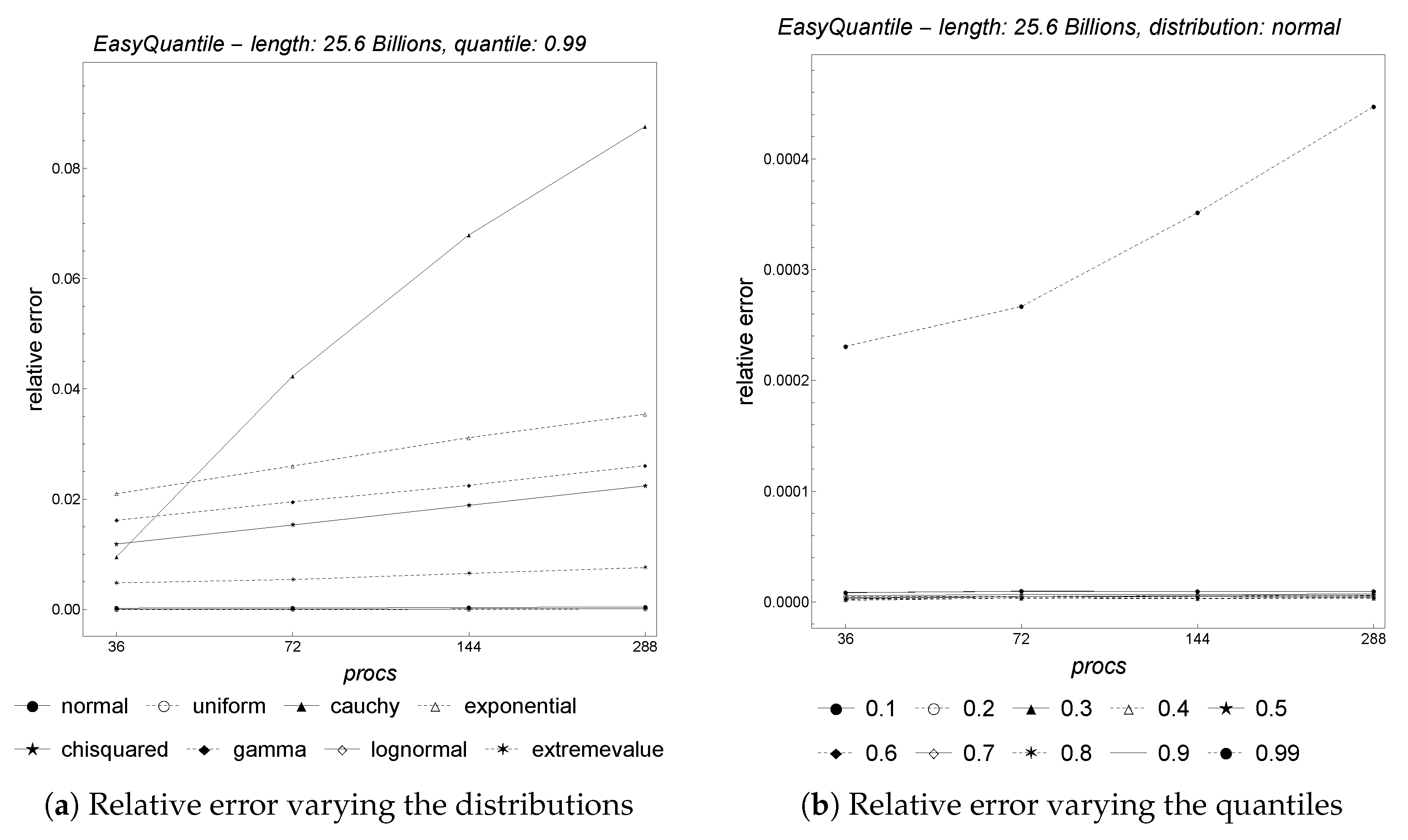Finally, the accuracy depicted in Figure 12 is extremely good for both distributions and quantiles.

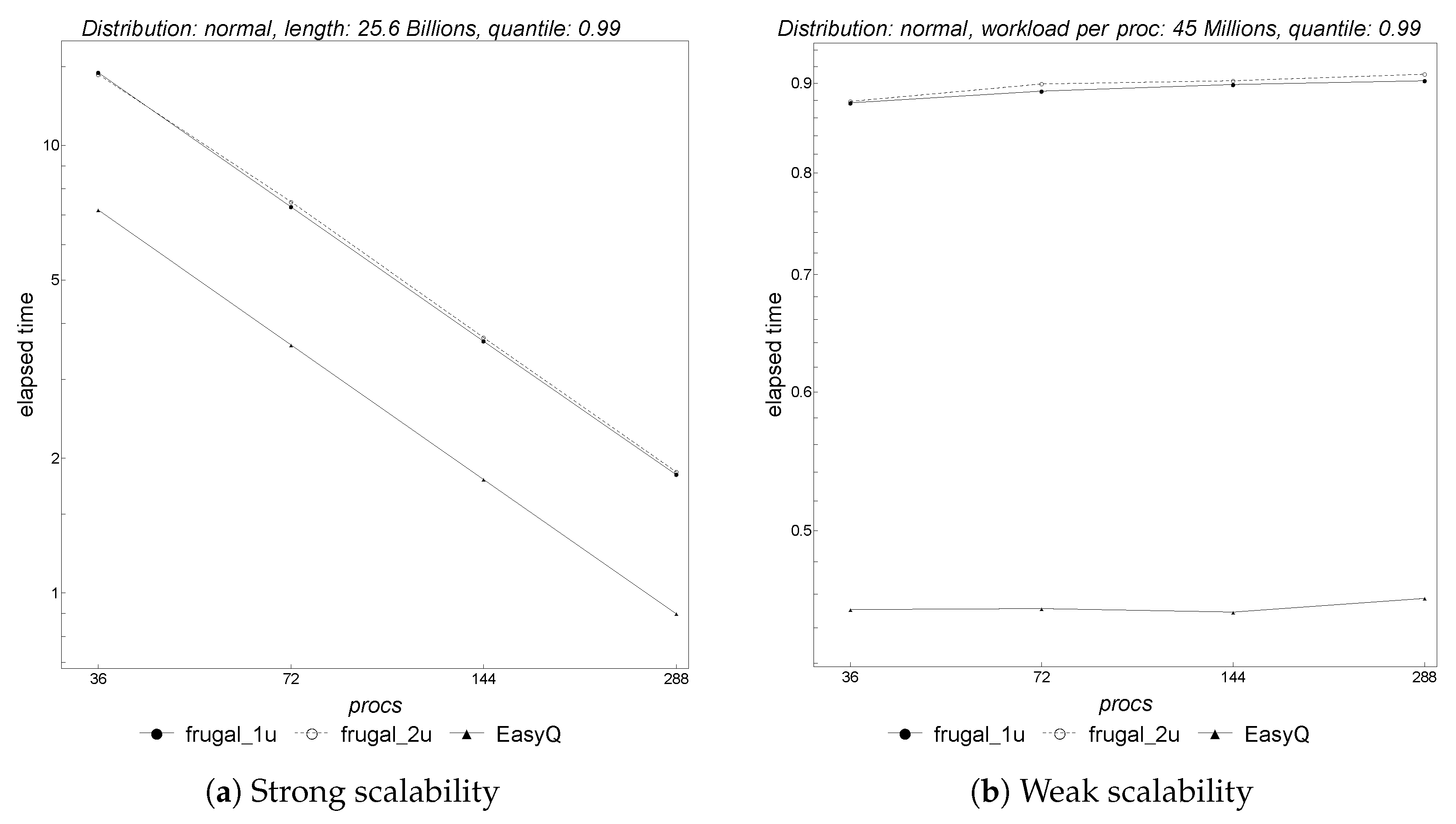
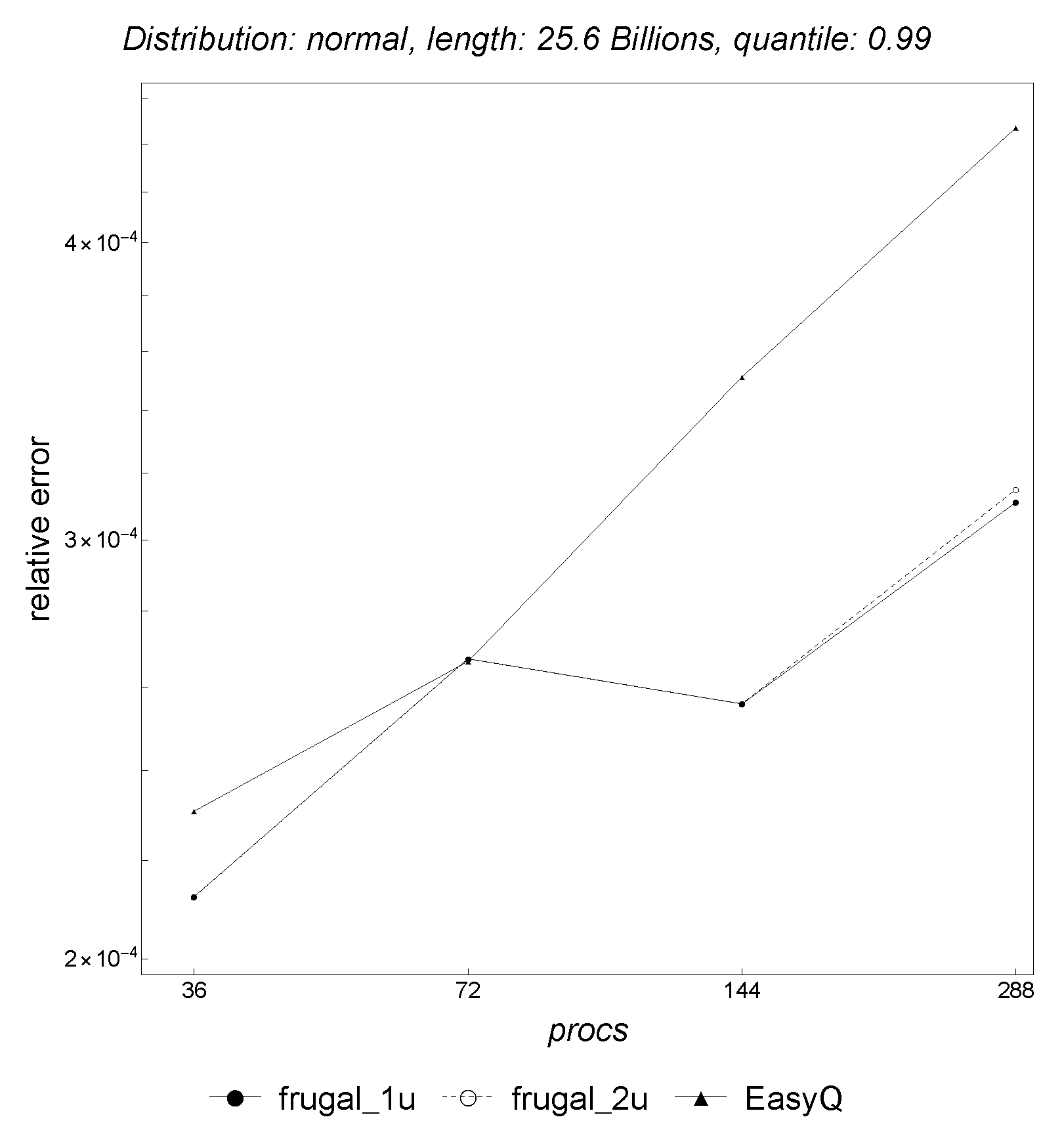
Having discussed the parallel algorithms’ results in isolation, we now turn our attention to selected experimental results, in which we simultaneously compare all of the parallel algorithms with regard to the normal distribution.

As shown in Figure 13, EasyQuantile scales much better than Frugal-1U and Frugal-2U with regard to both strong and weak scaling. Regarding the accuracy Frugal-1U and Frugal-2U are slightly better than EasyQuantile when tracking the 0.99 quantile, as shown in Figure 14.

We conclude that the parallel version of EasyQuantile is able to accurately track quantiles, especially higher quantiles, and provides the sought parallel performance as shown by the strong and weak scalability tests made. Therefore, it is the parallel algorithm of choice for tracking a quantile in a streaming setting, relying only on $O\left(1\right)$ memory.

7.2. Workstation

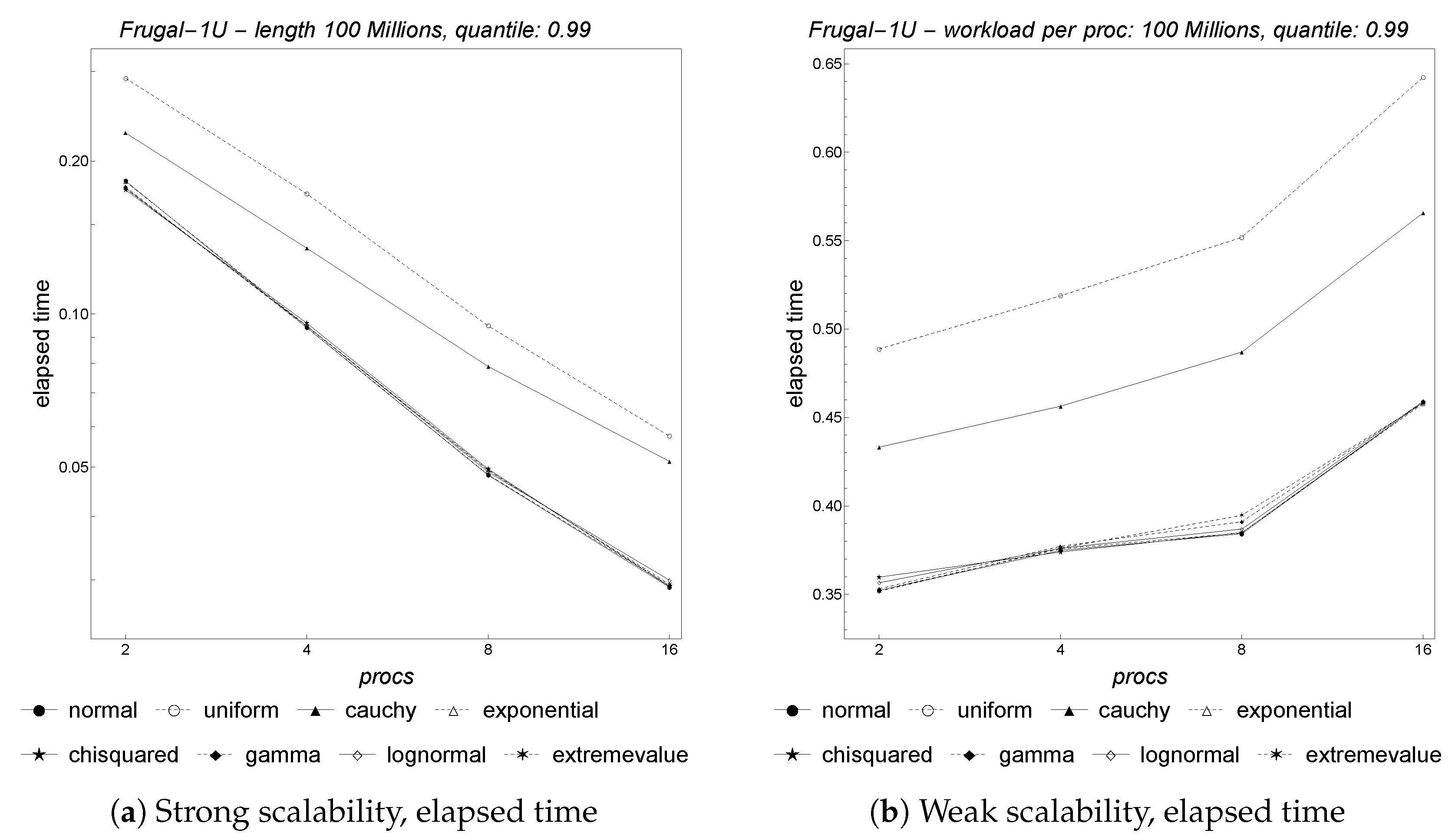
Here, we present the experimental results obtained on the HP workstation, using 2, 4, 8, and 16 cores. Figure 15 depicts the results related to the strong and weak scalability of parallel Frugal-1U. As shown, the algorithm scales until 8 cores, then the upward curvature for 16 cores indicates limited scalability. Regarding weak scalability, the upward trend of the curves indicates limited scalability as well. This is not really surprising, owing to the fact that the workstation has not been designed for HPC (high-performance computing), whilst the architecture of a parallel machine is—instead—specifically designed for HPC. Even though the workstation may certainly be used for this purpose, we can not expect the same performance level. To better understand the gap between the parallel machine and the workstation, we also recall here that the former provides weak scalability using only 45 million items per core, whilst the latter does not provide weak scalability even using 100 million items per core, more than double the amount of data used for the parallel supercomputer.

Next, we analyze the relative error of parallel Frugal-1U. Figure 16 provides the results varying, respectively, the distributions and the quantiles. We observe that for almost all of the distributions, the relative error is quite low and close to zero. Only the uniform and the cauchy distributions exhibit high relative error, since the estimates obtained by each processor are already affected by a sufficiently high relative error, owing to the small size of the sub-stream assigned to each processor, which does not allow achieving a good estimate (lack of convergence). Regarding the quantiles, varying the processors does not affect the accuracy; indeed, the corresponding relative errors are very close to zero and do not change significantly by varying the cores.

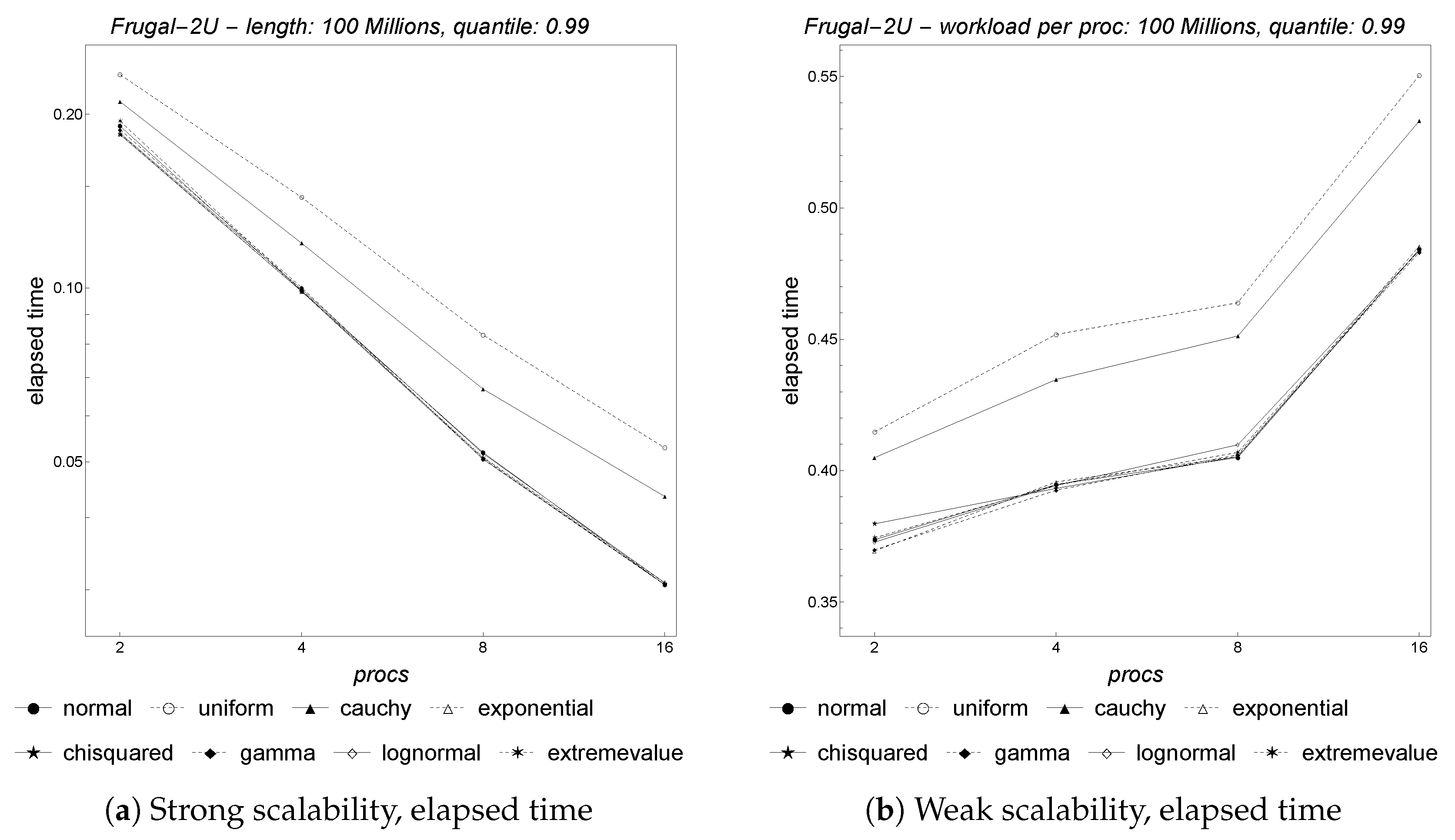
The parallel Frugal-2U presents the same behavior, as shown in Figure 17 and Figure 18, respectively, for strong/weak scalability and for the accuracy with regard to distributions and quantiles. In particular, parallel Frugal-2U achieves slightly better accuracy results with regard to parallel Frugal-1U, but is not significantly better overall.

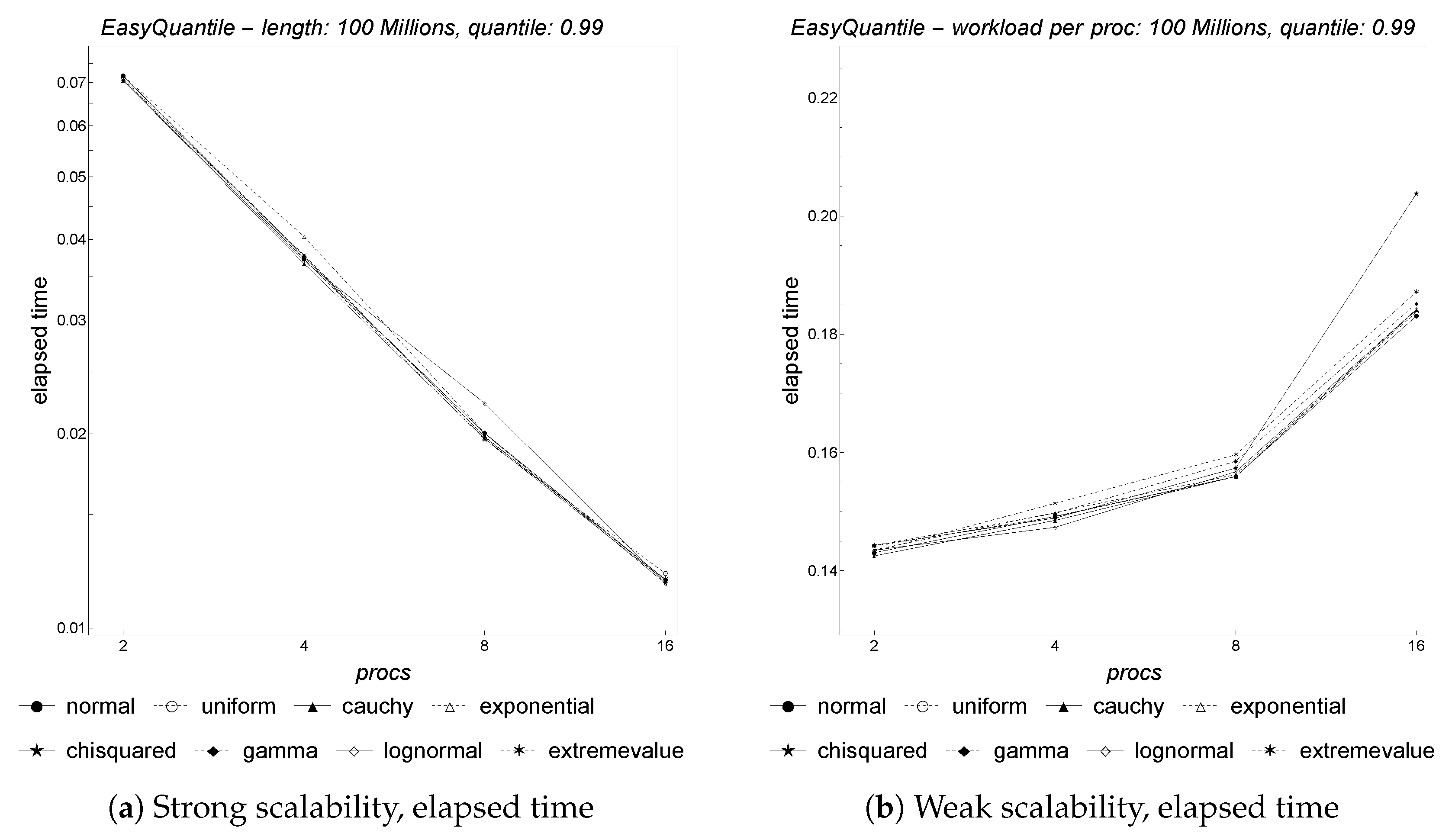
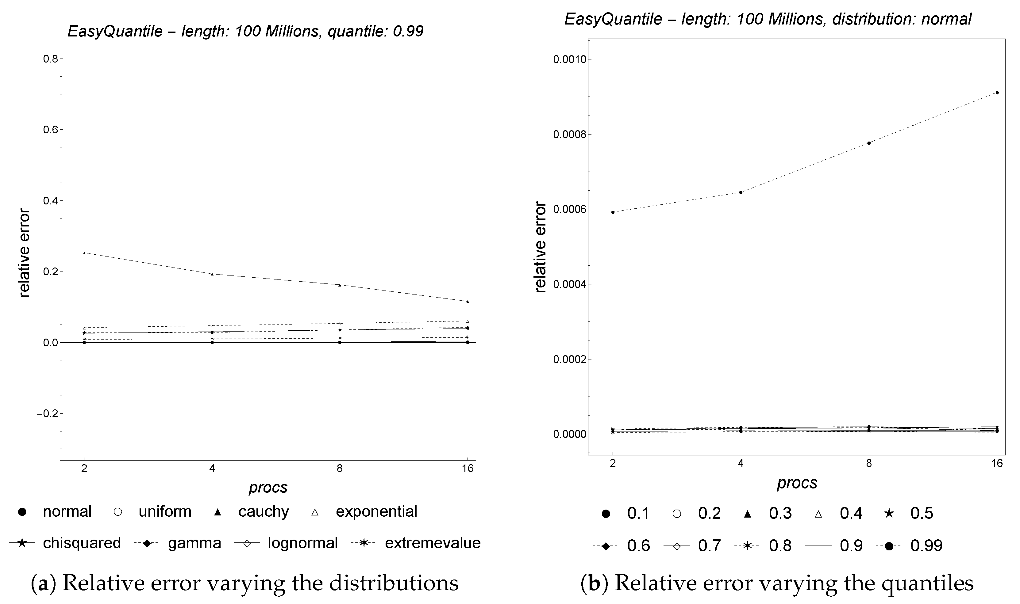
Finally, we discuss the results obtained by parallel EasyQuantile. Figure 19 depicts the strong and weak scalability of the algorithm. As shown, the algorithm is characterized by good strong and weak scalability, taking into account that the overall range of elapsed time is quite small for the weak scalability case. The accuracy, depicted by Figure 20, confirms that the parallelization does not impact on the relative error, whose values are close to zero and practically constant for all of the distributions and quantiles varying the number of processors (even though the curve related to quantile 0.1 appears to be slightly increasing, the range of variation is less than ${10}^{-3}$).

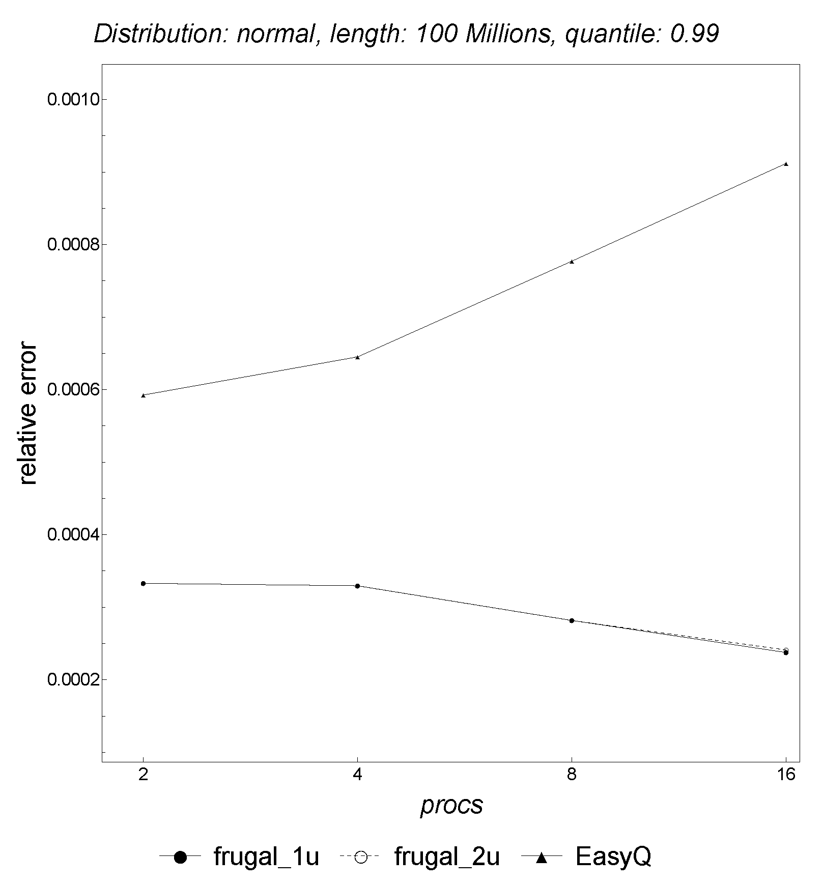
We end this section by comparing the three parallel algorithms simultaneously. Figure 21 shows that EasyQuantile scales better than Frugal-1U and Frugal-2U with regard to both strong and weak scalability. Regarding the accuracy, Figure 22 shows that Frugal-1U and Frugal-2U provide slightly more accurate results in terms of relative error. Overall, the results are quite similar to those obtained on the parallel supercomputer.

8. Conclusions

In this paper, we discussed the problem of monitoring network latency. This problem arises naturally in the context of network services such a web browsing, voice and video calls, music and video streaming, online gaming, etc. Since a high value of latency leads to unacceptably slow response times of network services, and may increase network congestion and reduce the throughput, in turn disrupting communications and the user’s experience, we discussed how to monitor this fundamental network metric. In particular, a common approach is based on tracking a specific quantile of the latencies’ values, e.g., the 99th percentile. We compared three algorithms that can track an arbitrary quantile in a streaming setting, using only a limited amount of memory, i.e., $O\left(1\right)$ cells of memory. These algorithms are Frugal-1U, Frugal-2U, and EasyQuantile.

We discussed their sequential speed of convergence on synthetic data drawn from several distributions, then we designed parallel, message-passing based versions, and we also discussed corresponding distributed versions. We proved theoretically their cost-optimality by analyzing them, and compared their parallel performance in extensive experimental tests. The results clearly show that, among the parallel algorithms we designed, the parallel version of EasyQuantile is the algorithm of choice, exhibiting very good strong and weak scaling with regard to its parallel performance, and extremely low relative error with regard to the accuracy of the quantile estimate provided.