Abstract
Smart contracts are programs that reside and execute on a blockchain, like any transaction. They are automatically executed when preprogrammed terms and conditions are met. Although the smart contract (SC) must be presented in the blockchain for the integrity of data and transactions stored within it, it is highly exposed to several vulnerabilities attackers exploit to access the data. In this paper, classification and detection of vulnerabilities targeting smart contracts are performed using deep learning algorithms over two datasets containing 12,253 smart contracts. These contracts are converted into RGB and Grayscale images and then inserted into Residual Network (ResNet50), Visual Geometry Group-19 (VGG19), Dense Convolutional Network (DenseNet201), k-nearest Neighbors (KNN), and Random Forest (RF) algorithms for binary and multi-label classification. A comprehensive analysis is conducted to detect and classify vulnerabilities using different performance metrics. The performance of these algorithms was outstanding, accurately classifying vulnerabilities with high F1 scores and accuracy rates. For binary classification, RF emerged in RGB images as the best algorithm based on the highest F1 score of 86.66% and accuracy of 86.66%. Moving on to multi-label classification, VGG19 stood out in RGB images as the standout algorithm, achieving an impressive accuracy of 89.14% and an F1 score of 85.87%. To the best of our knowledge, and according to the available literature, this study is the first to investigate binary classification of vulnerabilities targeting Ethereum smart contracts, and the experimental results of the proposed methodology for multi-label vulnerability classification outperform existing literature.
Keywords:
smart contract; vulnerability; deep learning; KNN; RF; ResNet50; VGG19; DenseNet201; performance metrics 1. Introduction
Data integrity and security are needed with the increasing development of different systems and applications and the handling of large volumes of sensitive data across various applications [1]. The inception of blockchain technology in 2008 marked a significant milestone, particularly with Santoshi Nakamoto’s revelation of Bitcoin transactions [1]. This revolutionary technology constitutes a chain of blocks linked by cryptographic hashes, securing transactions with encrypted information and timestamps [1,2]. Blockchain’s decentralized and distributed ledger design ensures tamper-resistant data storage and trust in transactions across a peer-to-peer network [2,3]. However, the accessibility of sensitive transactions to all network participants has raised concerns about privacy and security [4,5]. To address these issues, the Ethereum platform introduced smart contracts in 2015, drawing inspiration from Nick Szabo’s 1994 proposal [6].
A smart contract is a program stored within the blockchain platform; like transactions, it enforces conditions, privileges, penalties, and access policies for transactions and other contractual terms that are agreed upon by the contract parties [7,8,9]. Smart contracts are executed automatically when the transaction owner’s predetermined conditions are met, enforcing transaction terms without needing a central authority or third-party guarantee [9,10]. Smart contracts give network automation and the ability to convert paper contracts into digital contracts.
Despite the recognized advantages of smart contracts and the positive impact of their use on blockchain applications, network security, and system performance, the gap in security challenges primarily targeting smart contracts is an obstacle to the complete optimization of smart contracts in blockchain applications [9,10,11,12,13,14]. The gap, which is primarily the vulnerability of incorrectly written smart contracts to exploitation, is high, underscoring the need for a focused effort on secure cryptographic practices [9,10,11,12,13,14]. Attackers exploiting vulnerabilities in smart contracts have led to failures in blockchain systems [15,16]. For example, in 2016 the Decentralized Autonomous Organization (DAO) smart contract was manipulated to steal around USD 50 Million US at the time, due to its reentrancy vulnerability.
One way to discover and verify these vulnerabilities is utilizing instruction-based tools. These tools may assist in writing correct smart codes; however, they cannot find all vulnerabilities targeting smart contracts [17,18]. Therefore, there is still a need for more comprehensive solutions to detect and address various security threats targeting smart contracts. Classifying vulnerabilities is an important issue that helps in their detection and facilitates the search for other vulnerabilities. In the future, smart contracts are expected to be the most important component of blockchain optimization [9,19].
This paper uses deep learning algorithms, a powerful tool in data analysis, to detect and classify vulnerabilities targeting smart contracts. The deep learning algorithms, namely VGG19, ResNet50, KNN, Random Forest, and DenseNet201, are used for binary classification to ascertain whether any smart contract (represented as an image) contains a vulnerability or not, and for multi-label classification to determine the presence of one or more vulnerabilities indicating their type(s). For the two types of classification used, two smart contract datasets are used, which contained 12,253 smart contracts labeled with vulnerabilities and non-vulnerabilities [20,21], and one of them is the first real-world labeled dataset.
The main objective of this study is to strengthen the security of smart contracts and create a more robust blockchain network by detecting and classifying eight different vulnerabilities using five deep learning algorithms and experimentally assessing them in terms of accuracy, F1-score, Precision, Recall, and execution time. As part of our contribution, we hope to emphasize that instruction-based tools now in use for detecting and addressing attacks, vulnerabilities and threats targeted at smart contracts are not as efficient and capable of detecting unknown and more sophisticated attacks and suffer from lack of flexibility and long detection time. In addition, we highlight the best algorithm for binary and multi-label classification to detect and classify efficient vulnerabilities in smart contracts, by categorizing a dataset that contains 12,253 smart contracts.
The main contributions of this study to the field of smart contract vulnerability detection and classification using deep learning include the following:
- Novelty in Binary Classification: to the best of the author’s knowledge, this study is the first known research to explore binary classification for Ethereum smart contract vulnerabilities using deep learning algorithms.
- Effectiveness in Classification Approach: to the best of the author’ knowledge, and according to experimental results, this study outperforms the currently available literature on multi-label classification for Ethereum smart contract vulnerabilities using deep learning algorithms.
- Real-world Dataset and Algorithm Evaluation: this work utilizes a novel, real-world smart contract dataset for classification using five deep learning algorithms (ResNet50, VGG19, DenseNet201, KNN, and RF). This allows for a comprehensive evaluation of their effectiveness based on real-world data
- Innovative Data Representation: this research introduces a unique approach of converting smart contracts’ bytecode into RGB and grayscale images. Then, the effectiveness of this image conversion process in achieving optimal accuracy and F1-score for vulnerability detection is verified.
This paper is organized as follows. In Section 2, the relevant previous literature is listed, and the requirements of this research, including the concepts and resources used, are stated. Section 3 describes the proposed models for binary and multi-label classification and the explanation and representation of the dataset used for images and features. Section 4 highlights the presentation and discussion of the results and the proposed models. Finally, concluding remarks and recommendations for future work are emphasized in Section 5.
2. Related Work
Smart contracts are crucial in modernizing transactions, spurring in-depth exploration of their features and vulnerabilities. These contracts possess vital attributes that highlight their significance across diverse applications. Immutability, a central aspect, ensures that once a smart contract is published, it remains unaltered, demanding thorough verification before deployment—a departure from the adaptability of traditional contracts [17]. The owner empowers transaction creators to set privacy and access policies, and the specific conditions outlined in smart contracts enhance system performance [14,22]. Additionally, smart contracts boost security by addressing blockchain limitations, imposing conditions, and restricting unfettered access to network transactions [17]. They also enhance privacy by limiting access to contract contents solely to parties bound by specified conditions [18,22]. Moreover, the cost-effectiveness of smart contracts, compared to traditional counterparts, enhances their attractiveness by reducing preparation and implementation expenses. These contracts instill heightened confidence and trust among system parties, and their efficient access control mechanisms outshine capability-based systems, underscoring the diverse benefits smart contracts bring to transactional ecosystems. However, smart contracts are susceptible to various vulnerabilities which can lead to massive exploit, data, and fund losses. Below are the vulnerabilities that will be addressed in this work:
- (a)
- Arithmetic (ARTHM): Defines the integer overflow/underflow. An Arithmetic vulnerability occurs when an arithmetic operation in a smart contract exceeds a type’s maximum or minimum size. This type of vulnerability occurs when an arithmetic operation creates a numeric value that can be represented by a certain number of bits out of the range so that the values are set up to the maximum or minimum size of the representable value. The attacker can exploit the Arithmetic vulnerability and change the behavior of the smart contract unexpectedly, which leads to tampering with the smart contract or performing unauthorized actions [23,24].
- (b)
- Denial of Service (DoS): Smart contracts are categorized based on two types of DoS: DoS with a Failed Call and DoS Block Gas Limit. DoS with Block Gas Limit occurs when the gas limit specified for the block set by the Ethereum network is exceeded. Each function or procedure within smart contracts has a certain amount of gas that should not be exceeded when executing these functions or deploying smart contracts. DoS with Failed Call represents the failure (intentionally or unintentionally) to make external calls, and this usually occurs when there are many calls in the same single transaction [15,25,26].
- (c)
- Locked Ether (LE): A payable function increases the balance of the contract from ether so that when the contract is executed, the funds are reserved without being paid. This will not allow the expected ether to be received due to the job’s execution. Such vulnerabilities occur on private Ethereum contracts [16,27].
- (d)
- Reentrancy (RENT): A recursive call attack that occurs during the execution of the first call to the function so that the malicious contract invokes the call contract before the execution of the first call is completed. Invitations within a function can cause it to interact in undesirable ways [16,28].
- (e)
- Block values as a proxy for time (TimeM): In some cases, unsafe values, such as “block. number” and “block. timestamp”, are used to obtain the time values that some functions need to be executed. In smart contracts, such values can provide an idea regarding the current time or time delta between blocks required to trigger events. Since the block time is not constant and provides no precise values, this may create unexpected effects [29].
- (f)
- Transaction Order Dependence (TimeO): The vulnerability is caused by Ethereum’s block processing, where miners prioritize transactions with high gas prices. Transactions sent to the network are distributed to nodes for processing, allowing node operators to predict their order. A race condition vulnerability occurs when code relies on the transaction sequence, which will impact the outcomes. In addition, this matter is frequently and significantly repeated with rewards or approvals, as it leads to unintended token transfers, which happens in ERC20 tokens [30].
- (g)
- Unchecked Call Return Value (UE): This vulnerability occurs when the return values from different calls are not checked in the smart contract code, mainly when low-level calling methods are used. The effect of this vulnerability is that the call fails by mistake or intentionally because of the attacker who exploited its presence, in addition to an unexpected change in behavior [31].
- (h)
- Authorization through tx-origin (TX-Origin): This vulnerability occurs when returning the account address that sent the transaction and authorizing the “tx.origin” variable to return it. The “tx.origin” is a variable found in Solidity, and its purpose is to return the account that sent the transaction. However, using the “tx.origin” variable is not secure, and risks the smart contract. This may be due to sending another address of a malicious smart contract instead of calling the account address that sent the transaction. This could change the behavior of the smart contract unexpectedly [32,33].
Classification and Detection of Vulnerabilities in Smart Contracts
Vulnerabilities in smart contracts can be classified and detected based on more than one input format such as source code, byte code, opcodes, and images. Moreover, previous studies have dealt with the use of some forms of smart contracts and the impact of using this form on the results of discovering vulnerabilities. However, few studies have taken it upon themselves to study the classification of vulnerabilities using deep learning [9,34,35].
In Ethereum, an opcode (operation code) refers to the fundamental operation that the Ethereum Virtual Machine (EVM) can execute [36]. Each opcode corresponds to a specific operation, such as arithmetic, stack manipulation, or control flow. However, the bytecode is the low-level representation of a smart contract composed of opcodes (a series of opcodes) and their operands [36].
Soud et al. [35] introduced an automated framework for mining and classifying vulnerabilities in smart contracts. Utilizing a 4.4 KB primary dataset from CVE records and the NVD database, the framework addresses security vulnerabilities in two stages. Firstly, dynamic analysis techniques are employed to mine vulnerabilities in Ethereum smart contracts, monitoring their real-time behavior during execution. In the absence of execution, only the source code undergoes analysis. Subsequently, the mined vulnerabilities are classified based on Ethereum smart contract characteristics, impact, and patterns, ensuring a systematic approach. Notably, the framework goes beyond identification and classification, providing practical solutions to address and mitigate vulnerabilities within each identified category, reinforcing the robustness of smart contracts.
Jianga et al. [37] proposed a method for categorizing smart contracts in decentralized applications (DApps) related to blockchain-based cyber–physical systems (CPS). Using characteristics taken from smart contract data, such as contract address, creation date, and invocation details, this method uses the same classification system as DApps. The process uses three feature kinds (value, code, and time) from 5659 DApps acquired using DappRadar, Ethereum, and the State of the DApps. These features are used to construct feature vectors, which are then fed into a DApp classification model that uses KNN, XGBoost, and random forests, based on an integrated taxonomy. Although several accuracy values were obtained, 0.886727 was the highest performance attained.
Khodadadi et al. [38] utilized the ScrawlD dataset, comprising 6780 labeled smart contracts, and incorporated a partially labeled dataset from smartBug. Unnecessary elements like comments and spaces were removed during dataset preprocessing, retaining crucial words in the smart contract source code. Two inputs were employed: the source code and Opcode (compiled source code instructions). The WEM process converted the source code to a matrix based on characters for neural network compatibility. FastText and BiGRU were employed for word embedding, representing each word as n-grams and extracting features. Serialization combined features into a layer, contributing to a classification accuracy of 79.7%.
Rossini et al. [39] investigate the use of several Convolutional Neural Networks (CNNs) and a Long Short-Term Memory (LSTM) neural network in the application of deep learning to the classification of vulnerabilities in smart contract code. After considering five different vulnerability classes, the findings show that CNNs encourage accuracy, confirming the viability of the suggested approach. The study shows that vulnerabilities in smart contract programming may be efficiently found and categorized using deep learning techniques. After training and testing four neural network architectures, the 1D ResNet CNN produced the best results in terms of accuracy, 73.5%, and Micro F1 scores, 83.3%, when applied to smart contract bytecodes. The low performance of the LSTM baseline was probably caused by bytecode truncation. Due to the patterns in Solidity code, 2D CNNs (ResNet, Inception) were less successful in identifying vulnerabilities, even if they did not require truncation. The ResNet 1D convolutional network produced the best overall performance with a longer maximum length, necessitating input cutoff.
Hu et al. [22] studied how to deal with Ethereum smart contract challenges, focusing on fraud, vulnerabilities, and redundant contracts that affect performance. They introduce a transaction-based classification and detection method using 10,000 Ethereum smart contracts. The manual analysis identifies four behavior patterns, translated into 14 features. A data-slicing algorithm constructs the experimental dataset and presents a methodology for Ethereum smart contract classification using the LSTM network. They also measure security, performance, and contract management using performance metrics. The proposed approach achieves an F1-score of 0.77, a precision of 0.88, and a recall of 0.70.
In this research, we will present a different methodology for using deep and machine-learning algorithms in classifying and detecting vulnerabilities. Five algorithms were used to study their impact on binary and multi-label classification processes. There is no reason for choosing these algorithms over others, but the features of these algorithms that will be explained in the methodology section are the reason for testing them. It is possible to apply any algorithm to the proposed methodology.
From the author’s point of view, the shortcomings of instruction-based tools are what made studying the impact of deep learning on discovering and classifying vulnerabilities in smart contracts a matter of great importance, especially due to its promising performance and capabilities in industry and academia. For example, the suffering of instruction-based tools from low efficiency, low automation, and long detection times necessitates a comprehensive tool that can overcome these shortcomings. Deep learning algorithms can make up for the problems of instruction-based tools. Therefore, this hypothesis is the basis on which our research is based.
3. Methodology
The shortcomings in the tools used to discover and address vulnerabilities targeting smart contracts are that they do not detect all vulnerabilities, but rather detect a maximum of 4 or 5 types of vulnerabilities. This is what some previous studies have suggested [1,4,5]. Therefore, one of the best alternative solutions that can be used is to study the detection and classification of vulnerabilities targeting smart contracts by machine learning. This section describes the datasets used, the conversion process to images, and the algorithms used for detection and classification processes.
3.1. Preparation of the Dataset
3.1.1. Datasets Used
- The ScrawlD dataset, comprising 9253 smart contracts, represents the first real-world dataset labeled for vulnerabilities. There were two phases to the labeling process: the first phase included 6780 labeled smart contracts, and the second phase, which took place a few months later, had 9123 labeled smart contracts [20]. Five distinct tools were used, each with various versions and dependencies, making it difficult to label the full dataset at once and creating compatibility problems [20]. The Mythril tool’s large memory usage—roughly 10 GB—also made things more difficult [20]. The process of labeling smart contracts for vulnerabilities requires using tools like smart-check and Mythril. The “majority of results” standard was used, which means that if two or more tools found a vulnerability, it was confirmed to be present. Furthermore, this process consumes a lot of time. The dataset, and its labeled vulnerabilities, are publicly available on GitHub [40].
The ScrawlD dataset has been labeled with vulnerabilities described earlier. In addition, each smart contract could contain one or more vulnerability based on the results of the tools discovering these vulnerabilities, as shown in Figure 1, where the second contract, for example, contains both the LE and RENT vulnerabilities.

Figure 1.
A sample of ScrawlD dataset.
- The Slither dataset is an extensive assemblage of 35,000 smart contracts that represent the heterogeneous terrain of Ethereum-driven applications. The Slither dataset has been labeled based on no-vulnerabilities and vulnerabilities, Shadowing, Uninitialized variables, Suicidal Contracts, and arbitrary sending of ether vulnerabilities and safe smart contracts. Interestingly, this work used a sample of this dataset, which included 3000 smart contracts with safe labels (no vulnerability) [20]. The choice of contracts with safe labels emphasizes the need to find security flaws and vulnerabilities in the bytecodes. This was made possible in large part by the Slither tool, which was created as a platform for static analysis of the Ethereum smart contract [21].
Developers can utilize the Slither tool’s output, which gives them clear and useful information about potential vulnerabilities. Using this information, the Slither tool helps to strengthen the resilience of decentralized apps on the Ethereum blockchain by proactively identifying and resolving vulnerabilities during the development phase, hence improving the security posture of smart contracts [20]. The Slither dataset is available in Hugging Face [41]. In addition, each smart contract in the Slither dataset could contain one or more vulnerabilities or be safe, based on the result of the Slither tool discovering these labels, as shown in Figure 2.

Figure 2.
A sample of secure smart contracts in the Slither dataset.
The datasets used are unique to the Ethereum platform due to several factors, including the availability of publicly available datasets compared to other platforms, the strong developer community on the platform, and the fact that it is public and more reliable than other platforms due to its longevity, security, and stability. Furthermore, Ethereum is currently the most popular development platform for smart contracts. To the best of our knowledge, there is no real-world labeled dataset available other than the ScrawlD dataset used in this study [19]. However, the methodology for binary classification, multi-label classification, and proposed approaches could be extended to other blockchains such as Exonum or Hyperledger Fabric.
3.1.2. Extraction
The ScrawlD dataset contains smart contract addresses and labels. The bytecodes for smart contract addresses were extracted from Etherscan [42]. This is achieved using an API key that is set from the Etherscan site itself. Also, Bytecodes in the Slither dataset were extracted directly from the Hugging Face [41], from which 3000 bytecodes were extracted, which are the safe ones.
3.1.3. Contract Filtering and Selection
The ScrawlD and Slither datasets in their default form cannot be used, because they have an unbalanced nature and contain a lot of information that is unnecessary for the classification and detection processes. The content is modified by deleting some Solidity bytecodes whose file’s length is empty [43,44]. This will help to enhance the accuracy of the classification results. Based on that, the combined dataset consists now of 11,858 samples, 8933 of which come from the ScrawlD dataset (all are vulnerable), and 2925 come from the Slither dataset (all are invulnerable).
3.1.4. Image Representation
To efficiently represent binary image data, the combined ScrawlD and Slither dataset was converted into RGB and grayscale images with a constant size of 224 by 224 pixels using Base64 encoding. To ensure flawless conversion, the process comprised reading RGB data files, encoding them with Base64, decoding the resulting binary data to produce RGB values, and parsing the binary data again to make sure they match their original bytecode counterpart. To ensure homogeneity through reshaping, the image dimensions were selected at 224 by 224 pixels based on data length. This procedure produced a standardized dataset by following the requirements of the deep learning model. Figure 3 displays some of the RGB images corresponding to some smart contracts’ byte codes.
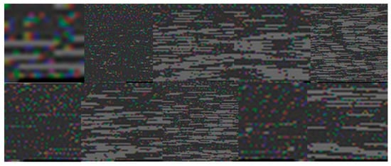
Figure 3.
Sample RGB images.
The same process is followed to generate grayscale images with dimensions determined by the binary data length and to resize the images to a uniform 224 × 224-pixel size. Figure 4 displays some of the grayscale images.
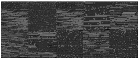
Figure 4.
Sample Grayscale images.
3.2. Binary Classification
The process of binary classification determines whether a smart contract has a vulnerability, i.e., each contract is classified as either “secure” or “insecure”. A subset of the ScrawlD dataset containing 2925 contracts was taken to match the number of samples in the Slither dataset. Figure 5 shows some samples from the dataset used in binary classification.

Figure 5.
Sample of the dataset used in Binary Classification.
The dataset, which contains 5850 contracts, was divided into three parts: 20% of each dataset class was allocated to the test set, 70% of each class was allocated to the training set, and 10% to validation. Then, these subsets were utilized to study the deep learning algorithms KNN, RF, ResNet50, VGG19, and DenseNet201. Figure 6 shows the distribution of the dataset used in binary classification. All proposed models in binary classification (and later multi-label classification) were trained with a maximum of 100 epochs and a batch size of 32. The early stopping method was also used, as it was set to stop training when the required performance metric (binary cross-entropy loss in this case) does not enhance for a duration of five epochs. The goal of linking the early stopping method to the binary cross-entropy loss is because the increase in loss greatly affects the incorrect prediction of the result of the smart contract classification, whether the smart contract is safe or unsafe, and the type of vulnerability present, so that it leads to misclassification.
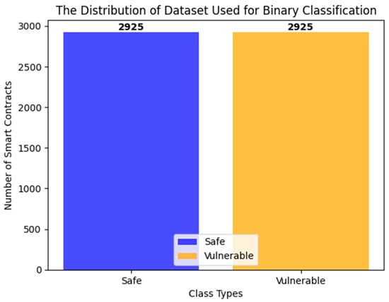
Figure 6.
The distribution of the dataset used in binary classification.
3.2.1. Binary Classification Using VGG19
Our binary classification usingVGG19 model sets up and trains a deep-learning model using TensorFlow and Keras on a dataset of RGB and Gray-Scale images, leveraging the pre-trained VGG19 architecture. The Keras models that were used in this study took advantage of the scalability and scalability capabilities of distributed training across multiple Graphics Processing Units (GPUs) and Tensor Processing Units (TPUs) provided by TensorFlow, which allowed for faster training times [45,46]. Without a GPU, the training time could reach more than eleven times and may be stopped. Training may be interrupted due to exceeding the period allowed in Google Colaboratory [47], which cannot exceed twelve hours. All proposed models in binary classification are trained with a maximum of 100 epochs and 32 batch size. The early stopping method was also used, as it was set to stop training when the required performance metric (binary cross-entropy loss, in this case) does not enhance for a duration of five epochs
Our VGG19 model starts by setting up image data generators for training, validation, and test datasets, including extensive data augmentation for the training set to enhance generalization using an Image Data Generator. Also, an Image Data Generator is used in preprocessing and validation. However, for the test datasets, we just used preprocessing without augmentation. The VGG19 model, pre-trained on ImageNet, is the base model with its weights frozen to retain learned features. A new sequential model is built on top of VGG19, consisting of a flattened layer to lower the spatial data that the convolutional layers have learned so that the fully connected layers may process it for ultimate classification and higher-order reasoning [48,49]. Also, the flattened layer is responsible for reducing the features extracted from convolutional and max pooling [48,49]. Additionally, the VGG19 model used a dense layer with 256 neurons and ReLU activation to enhance the network’s ability to learn and represent intricate features and patterns necessary for accurate classification, then used a dropout layer to prevent overfitting, and a final dense layer with sigmoid activation for binary classification.
The VGG19 model is compiled using the Adaptive Moment Estimation (Adam) optimizer with a specific learning rate of 1 × 10⁻⁵. The learning rate expresses a hyperparameter that determines the step size at each iteration while moving toward the minimumloss function. This Adam optimizer was used due to its ability to adapt to dealing with noisy or variable data sets, large data sets, and complex models, which contributes to improving model performance [49]. In addition, the loss function was defined as the binary cross-entropy expressing the difference between the predicted and true (target) probability distributions, and a few metrics like accuracy, precision, recall, and F1 score were specified to evaluate the model’s performance. When using VGG19 or any deep neural network architecture, the choice of optimizer, learning rate, loss function, and activation functions can greatly affect the training process and model performance. In the training and validation, the shuffle is set to true, but it is set to false in the test to ensure the test-data order remains the same for consistent predictions. Our Proposed VGG19 Model’s workflow is depicted in Figure 7.
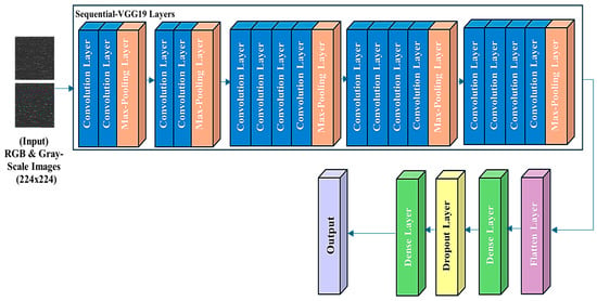
Figure 7.
VGG19 Model’s workflow.
3.2.2. Binary Classification Using ResNet50
ResNet-50 (Residual Network) is a pre-trained model of a Convolutional Neural Network (CNN). It consists of 50 layers: 48 convolutional layers, one MaxPool layer, and one average pool layer [50,51]. Keras was also used with ResNet-50 to transfer learning.
In our Binary ResNet50 model, the same structure and properties were used as in the VGG19 model. However, there is one difference, which is that the Global Average Pooling layer was used instead of the flattening layer because it is more suitable for the ResNet50 algorithm in terms of reducing the risk of overfitting and ensuring the model focuses on the presence of features rather than their exact locations, leading to potentially better generalization and performance for the classification task. Figure 8 shows the workflow of our ResNet50 model used.
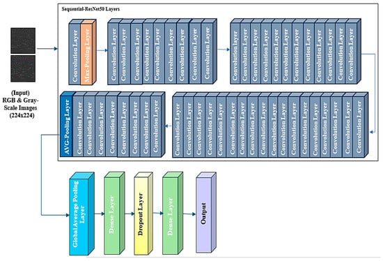
Figure 8.
ResNet50 Model’s workflow.
3.2.3. Binary Classification Using DenseNet201
The architecture of DenseNet201 contains 201 layers, including an initial convolutional layer followed by four dense blocks that contain a sequence of convolutional layers, separated by transition layers and ending with a global average pooling layer and a fully connected layer for classification. Also, the transition layers are allocated between two dense blocks and the transition layers are used to control the complexity of the model [52,53]. The workflow of our DenseNet201 model’s architecture is the same as that of the ResNet50 model; it is shown in Figure 9.
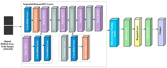
Figure 9.
DenseNet201 Model’s workflow.
3.2.4. Binary Classification Using Random Forests
RF builds multiple decision trees during training based on the number of trees and merges the outputs of each tree and their decisions to improve the predictive performance and control overfitting [54]. RFs are usually trained with the bootstrapping method, a combination of learning models that increases the overall result [55]. To prepare the images for training, they are converted to numerical arrays and split into training, validation, and test sets. Through bootstrapping, our RF model takes samples repeatedly from the same group of sets to estimate how accurate the estimates are. Then, a Random Forest classifier is initialized to train on the training set and validated using the validation set with varying numbers of trees by calculating the accuracy of each tree. Finally, the best model is based on optimal validation accuracy.
In RF terminology, the ‘n_estimators’ parameter, which defaults to 100, specifies the number of decision trees the Random Forest should build. However, we iterate over a range of tree counts from 20 to 420, with increments of 20. This means the loop will train models with 20, 40, 60, 80, up to 420 trees. A new Random Forest classifier is instantiated for each tree iteration with the next n_estimators. For each n_estimator, the tree used must calculate the best validation accuracy to choose the optimal n_estimators of the tree or random forest using the validation set. Figure 10 shows the workflow of the architecture of our proposed RF model.
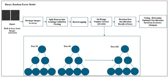
Figure 10.
Random Forest Model’s Workflow.
3.2.5. Binary Classification Using KNN
KNN relies on calculating the distance between instances, to make predictions. This study uses Euclidean distance to measure the straight-line distance between two points in a multi-dimensional space [49,56].
In our KNN Binary classifier, RGB and Gray-Scale Images are converted to numerical arrays to be classified using the KNN Algorithm. The default K-Parameter used initially equals 3, and K is considered the nearest neighbor to consider when making a prediction. However, when trained, the training set used a list of K-parameters, a range of odd numbers from 1 to 29, and chose the optimal value by calculating the validation accuracy utilizing the validation set. The choice of K-parameters significantly affects the algorithm’s performance.
For each k, a new KNN classifier is instantiated and then trained on the training data. Predictions are made on the validation set, and the accuracy of each prediction is calculated to choose the optimal k based on the best validation accuracy. Finally, the number of neighbors, the trained model, and accuracy are stored in their respective lists and plots. The trial approach helps find the optimal balance between underfitting and overfitting. Figure 11 shows the workflow of the binary classification architecture of our proposed KNN model.

Figure 11.
KNN Model’s workflow.
3.3. Multi-Label Classification
In this task, only the ScrawlD dataset, which contains 8933 smart contracts, is used, and all these contracts are labeled as containing one or more vulnerabilities. The dataset includes 8 of the vulnerabilities that were explained earlier in Section 2. They are ARTHM, DOS, RENT, TimeM, TimeO, UE, LE, and TX-Origin. Figure 12 shows a sample of the Dataset used.

Figure 12.
Sample of Multi-Dataset used.
After excluding 190 specific null byte codes from the dataset, the number of bytecodes becomes 8933. As a result, the distribution of vulnerabilities in the database will be changed. The “ARITHM” vulnerability frequency becomes 8568, while “RENT” is present in 5037 smart contracts. The remaining vulnerability frequencies are 2176, 1673, 1247, 1052, 1033, and 232, respectively, for “TimeM”, “LE”, “DOS”, “TimeO”, “UE” and “TX-Origin”, as shown in Figure 13.
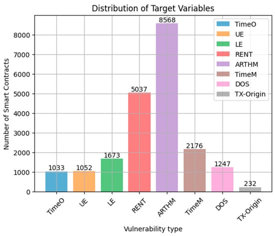
Figure 13.
Distribution of the labels after removing the specified bytecodes.
As shown in Figure 13, the distribution of classes in the multi-dataset is unbalanced, as there is an apparent disparity in the frequencies of smart contracts within each class. This is why it was necessary to use one of the methods of balancing datasets in deep learning. In this work, we defined a “balance” function to balance the dataset by sampling groups of under-represented classes. One sampling strategy used for imbalanced datasets is adding more examples from the minority class (oversampling) [57]. It was done by collecting all the labels in one list to facilitate processing and simplify the balancing process so that each unique set of labels is treated as one class [57]. Then, the maximum number of occurrences of any set of labels is determined, to use this value to determine the target size for oversampling [57].
Based on these occurrences, it replicates the under-represented classes over each set that share the same set of labels. For each set, it samples the tuples (with replacement) until the set size matches the target size. Balancing through resampling strategies ensures that all unique sets of labels are represented equally in the training set, which helps improve the performance and fairness of machine learning models trained on this data [57].
The multi-label classification process was carried out using three different approaches to obtain the best results:
- (a)
- Approach 1: Multi-label classification using all the labels contained in the dataset. This method was carried out by using the eight vulnerabilities: ARTHM, DOS, RENT, TimeM, TimeO, UE, LE, and TX-Origin.
- (b)
- Approach 2: Multi-label classification with the deletion of labels with few repetitions. Four of the vulnerabilities ‘DOS, TimeO, UE and TX-Origin’ were deleted and replaced with one class under the name ‘Others’.
- (c)
- Approach 3: Multi-label classification with the deletion of low-accuracy labels. Four of the vulnerabilities ‘UE, LE, DOS and ARTHM’ were deleted and replaced with one class under the name ‘Others’. This makes the dataset used in this approach more balanced and, hence, gives better accuracy.
Multi-Label Classification with Deep Learning Algorithms Using the Three Different Approaches
Different algorithms for multi-label classification are applied to RGB and Gray-Scale images resulting from conversion of the dataset. The three approaches described earlier were also applied in each algorithm, to ensure the best results.
The same process for preparing the dataset and selecting the hyperparameters is followed as in the case of binary classification, except that we changed the batch size to 64. The dataset was also augmented to improve and generalize the results.
In addition, the structure of the model on which the images were trained is the same as in the binary classification shown in Figure 7, Figure 8, Figure 9, Figure 10 and Figure 11, with the three approaches explained earlier being applied to each algorithm to study the extent of the impact of these structures in the different approaches used. VGG19, ResNet50, and DenseNet201 include the addition of a pre-trained corresponding model as the base, a flattened layer, and a fully connected layer with 128 neurons. In addition, a dropout layer with a rate of 0.5 was added to prevent overfitting. Finally, a dense or output layer with a sigmoid activation function for multi-label binary classification was added. For RF and KNN, the same process was followed as in the case of binary classification. However, it was applied to the three approaches explained previously. Figure 14 shows the complete multi-label classification process, using the previously mentioned algorithms and the operations performed on the dataset as a balance, using resampling.
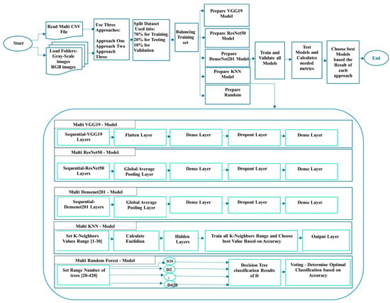
Figure 14.
Multi-Label classification processes.
3.4. Performance Metrics
Performance metrics such as precision, recall, accuracy, and F1-score are calculated to evaluate the effectiveness of the algorithms used in classifying instances with multiple labels and binary labels.
Confusion Matrix: The confusion matrix evaluates the performance of classification models by measuring metrics such as Accuracy, Recall, and Precision using values defined in Table 1. These metrics can be used to determine the success of the used model [58]. The confusion matrix also gives future insights into the maintenance, processing, and comparison of the models, to improve the classification.

Table 1.
Values of confusion matrix [58,59].
- Accuracy: This is one of the most popular metrics in multi-class classification. Accuracy represents the ratio of correctly predicted instances to the overall correctness of predictions, as illustrated in Equation (1) [58,59].
- Recall: This is the fraction between True Positive elements (correctly predicted positives) divided by the total number of positively classified units (all actual positives) [58,59].
- Precision: This is the fraction between predicted correct labels (True Positive elements) divided by the total number of positively predicted units [58,59].
- F1-Score: This is the harmonic meaning between precision and accuracy. Also, the F1-score is used to provide a balanced assessment of a model’s performance and handle the complexities introduced by the multiple labels in multi-label classification [60].
4. Results and Discussion
The ScrawlD dataset was used for binary and multi-label classification, while the Slither dataset was used for binary classification due to the subset that was taken, which are the safe smart contracts. Five deep learning algorithms were used to study the two datasets and then evaluate the performance of the deep learning algorithm models through performance metrics.
4.1. Results of Binary Classification
Table 2 presents the performance metrics of different algorithms based on binary classification to detect whether a vulnerability exists or not. The RF algorithm with RGB images achieves a high accuracy of 0.86666, an F1-score of 0.86666, a precision of 0.86635, and recall of 0.86671, indicating that it performs well in detecting a vulnerability. In addition, RF in Gray-scale images also performs well in detection tasks. However, it has a slightly lower accuracy and F1-score compared to RF with RGB. Specifically, it has an accuracy of 0.85641 and an F1-score of 0.85641. This shows that the RF algorithm, in general, is the best in terms of binary classification for smart contracts.

Table 2.
The performance metrics of models used in binary classification.
Also, the ResNet50 algorithm achieves a high accuracy of 0.84102, F1-score 0.84102, precision of 0.84437, and recall of 0.83926, indicating strong performance in vulnerability detection using RGB images. However, the ResNet50 algorithm shows good performance in vulnerability detection with grayscale images, although slightly lower compared to its RGB counterpart.
In the RF algorithm, which is considered the best algorithm in binary classification based on performance metrics, it took 9000 s in RGB images, while in grayscale images it took a longer time, reaching 9900 s, and achieved a lower F1-score accuracy of 0.01.
The confusion matrices in Figure 15, Figure 16, Figure 17, Figure 18, Figure 19, Figure 20, Figure 21, Figure 22, Figure 23 and Figure 24 show how well binary classification models are built using the various methods adopted. The model’s predictions for true negatives (TN), false positives (FP), false negatives (FN), and true positives (TP) are broken down in each confusion matrix.

Figure 15.
VGG19-RGB-Binary.

Figure 16.
VGG19-GRAY–Binary.

Figure 17.
ResNet50-RGB-Binary.

Figure 18.
ResNet50-GRAY–Binary.

Figure 19.
DenseNet201-RGB-Binary.
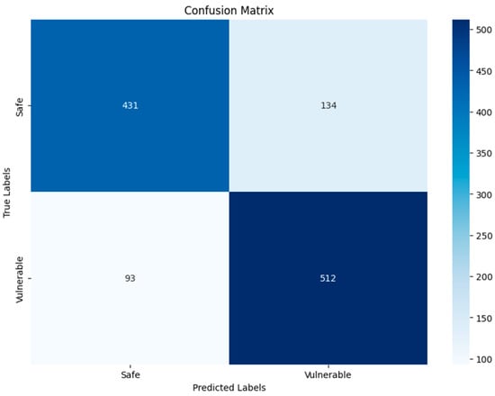
Figure 20.
DenseNet201-GRAY–Binary.
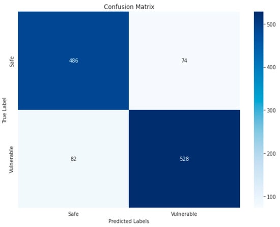
Figure 21.
Random Forest-RGB-Binary.
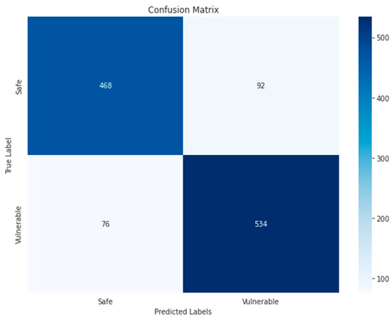
Figure 22.
Random Forest-GRAY–Binary.
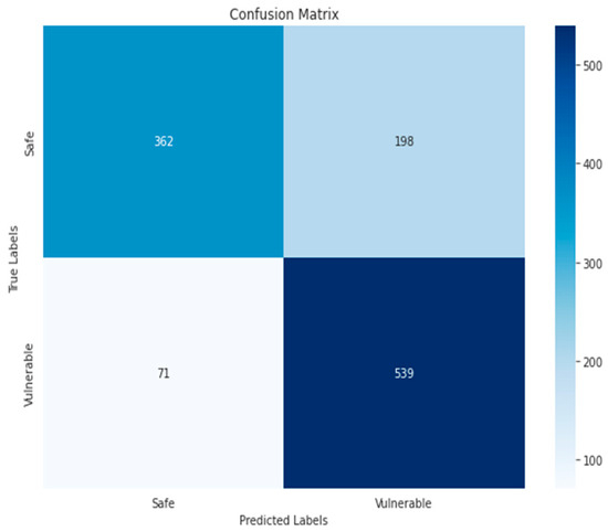
Figure 23.
KNN-RGB-Binary.
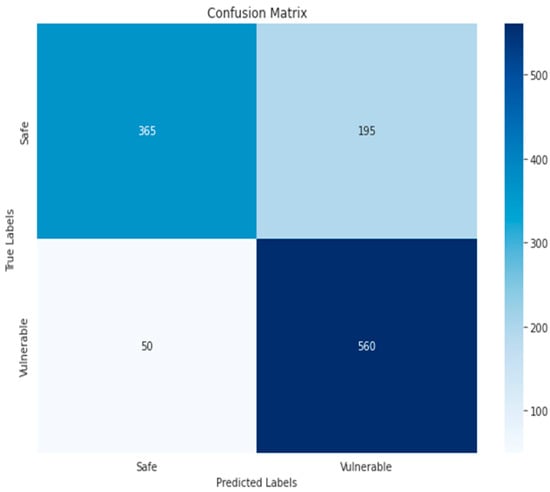
Figure 24.
KNN-GRAY-Binary.
In RF algorithm, the TP and TN in RGB images indicate that the model has detected correctly the largest number compared to other algorithm models, which reached 486 and 528, respectively, while TP and TN in grayscale images are 468 and 534, respectively. The reason for the superiority of the RF algorithm is that each RF tree calculates the importance of a particular feature according to its ability to increase the purity of the leaves while making classification trees. The greater the increase in the purity of the leaves, the greater the importance of the feature, which is well reflected in the classification results.
The confusion matrix of the KNN algorithm did not achieve satisfactory results, as is clear in Figure 23 and Figure 24, where the TP and TN for the RGB and grayscale images reached 362, 539, 365, and 560, respectively. The reason could be due to the sensitivity to choosing k. As for the ResNet50 algorithm, the increase in false positives (125) and false negatives (96) in Figure 18 indicates less accurate prediction performance. Compared to ResNet50-GRAY, Figure 17 shows an improvement in false positives (120) and a decrease in false negatives (66), and the ResNet50 algorithm with RGB images is the second-best algorithm for second classification.
As for the DenseNet201 and VGG19 algorithms for grayscale and RGB images, the increases in DenseNet201 TP, TN, FP, and FN were slight compared to VGG19, as shown in Figure 15, Figure 16, Figure 19 and Figure 20, where the DenseNet201 algorithm for both RGB and grayscale image types was as follows: 430, 533, 135 533, 431, 512, 134 and 93. Finally, the results of the confusion matrix of the VGG19 algorithm for RGB and grayscale images were 456, 481, 109, 124, 428, 533, 137, and 72. DenseNet201 results are better, due to the number of layers and to the nature of its structure being better than VGG19, which is considered unsuitable compared to DenseNet201 and the other algorithms used.
The results of RGB images being better than grayscale images in binary classification can be attributed to the richer and more detailed information provided by color channels. With their three-color channels—Red, Green, and Blue—RGB images can capture the subtle subtleties and complex color patterns that grayscale images, which only have one intensity channel, may be unable to capture. When the classification job depends on color-related features, this extra color information improves feature discrimination and enables the representation of intricate color patterns. Color information can transmit more complete and discriminative visual qualities which are important to the classification problem, which is generally why RGB is superior to grayscale. So, in image classification, RGB images are better than grayscale images, and the best algorithm is RF. The result of the f1-score is 0.86666.
4.2. Results of Multi-Label Classification
The multi-label classification in the context of vulnerability detection involves the classification of the multi-dataset into one or multiple classes. Five algorithms including RF, KNN, DenseNet201, VGG19, and ResNet50 were used in multi-label classification based on both RGB and grayscale images. These algorithms were investigated by applying the three approaches detailed in Section 3, to ensure the best and most accurate results. Each approach differs from the other by the nature of the dataset used. The second and the third approaches were applied to better balance the dataset and increase accuracy. The most important insights into the performance metrics of these algorithms and approaches are given in Table 3.

Table 3.
The performance metrics of models used in multi-label classification.
In terms of the first approach, where none of the labels were deleted while resampling was applied to obtain a balanced dataset, Table 3 shows that the RF algorithm based on RGB images has provided the best results. The obtained accuracy and F1-score results were 88.39% and 78.27%, respectively. The RF algorithm based on grayscale images has also achieved the second-highest performance metric and provided results almost like those of RGB images. Accordingly, RF can be considered as the best algorithm when considering all the labels of the multi-dataset. The VGG19 algorithm based on RGB images has achieved good results as well, and can be considered the second-best algorithm for this approach when performing multi-label classification. The accuracy and F1-score reached 86.43% and 76.46%, respectively. Yet, when applying this approach to grayscale images, the performance metrics were lower than those of RGB images. The accuracy declined to 80.61% and the F1-score to 67.64%. Hence, it is not possible to generalize that the VGG19 algorithm is suitable for the classification of all vulnerabilities. The results obtained based on ResNet50 were almost like VGG19-Gray. The DenseNet201 and KNN algorithms could not be trained using the first approach either on RGB images or grayscale images due to the prolonged time required for the training and the limitation of the available devices.
In terms of the second approach, where labels with few repetitions have been deleted and combined in one class called ‘Others’, Table 3 shows that the RF has again achieved clear superiority in this approach. The accuracy in grayscale images reached 88.18% and the F1-score 84.55%. As for the RGB images, there was a slight decrease, as the accuracy reached 84.25% and the F1-Score was 81.95%. VGG19-RGB and KNN based on both RGB, and grayscale images have achieved the second-best results after RF, with their accuracy and F1-score around 81.5% and 79%, respectively. The results of the remaining algorithms were around 74% for both accuracy and F1-score values.
In terms of the third approach, where low-accuracy labels have been deleted and combined in one class called ‘Others’, Table 3 shows that the VGG19 algorithm based on RGB images has provided the best performance metrics. An accuracy level of 89.14%, an F1-score of 85.87%, a precision of 85.09%, and a recall of 86.66% were achieved. This suggests that the VGG19 model trained on RGB images is particularly effective in identifying and classifying vulnerabilities within the dataset. Close performance metrics were achieved using RF-RGB, KNN-RGB, and KNN-GRAY algorithms. However, the results based on grayscale images for both VGG19, and RF algorithms appear to be lower compared to RGB images. The lowest performance was achieved using ResNet50 and DenseNet201 algorithms based on RGB images, with better results scored by ResNet50. Interestingly, for these two algorithms, their performance based on grayscale images was higher than when based on RGB images.
Considering the overall results, RF, KNN, and VGG19 algorithms consistently delivered strong performance metrics, with variations based on the approach and image type. Regardless of the used approach, RF and KNN algorithms maintained good performance across both RGB and grayscale images. In contrast, VGG19 excelled with RGB images, specifically in the multi-label classification using approach three. This suggests that VGG19 benefits from the richer information in RGB images for this specific task.
In multi-label classification, there is a difference in the time taken to train the algorithms and approaches used in this classification. The reason for that is due to several reasons, the most important of which is the difference in the dataset used each time the algorithm is trained, so that in the first approach, eight vulnerabilities are used. As for the second approach, only five vulnerabilities were used, because the four lowest vulnerabilities in the dataset were replaced with the “others” class. Similarly, in the third approach, in which four vulnerabilities with low accuracy were consolidated and replaced with “others”, five vulnerabilities were used.
The difference in the data set resulted in a difference in the training time. In addition, there is a difference in the number of layers in each algorithm and the pre-processing of the data. For example, in the first approach, RF in RGB images took 15,300 s, which is considered the best performance among all the applied algorithms. When using RF with grayscale images in the second approach, it took 8700 s. Finally, in the third approach, which represents replacing the four least-accurate vulnerabilities with the “other” class, this approach took the least time among all the used approaches. The best algorithm in the third approach is VGG19 with RGB images, which took 2160 s to train. This is because the models built by the algorithms learned well in less time.
The confusion matrices presented in Figure 25, Figure 26, Figure 27, Figure 28, Figure 29, Figure 30, Figure 31 and Figure 32 evaluate the performance of the best multi-label classification method using the RF algorithm in the first approach based on RGB images. The figures indicate high accuracy in vulnerability detection. In terms of ARTHM vulnerability, the largest existing vulnerability, Figure 25 indicates that 1714 out of 1722 ARTHM vulnerabilities were correctly classified (TN). Only 59 smart contract images were incorrectly classified (FP), and 10 images were ARTHM vulnerability (FN). Similar trends are observed for other vulnerabilities, regardless of their frequency, as shown in Figure 26 (RENT) and Figure 27 (TX-Origin). High numbers of correct classifications (TN) are seen, with a smaller number of misclassifications (FP and FN).
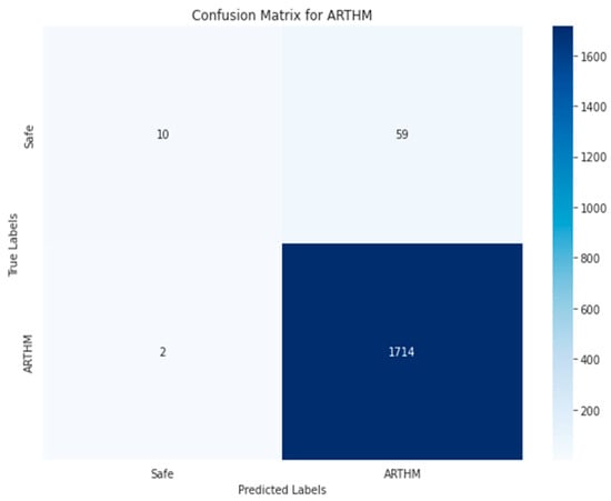
Figure 25.
Random Forest-RGB using Approach 1 for ARTHM class.
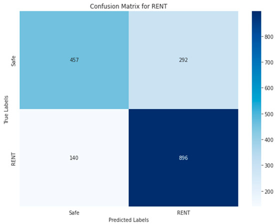
Figure 26.
Random Forest-RGB using Approach 1 for RENT class.
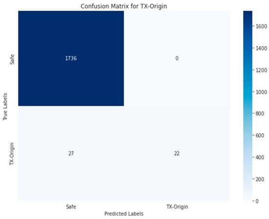
Figure 27.
Random Forest-RGB using Approach 1 for TX-Origin class.
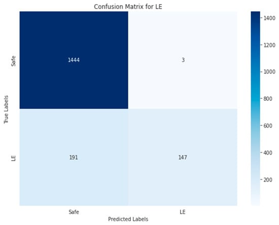
Figure 28.
Random Forest-RGB using Approach 1 for LE class.
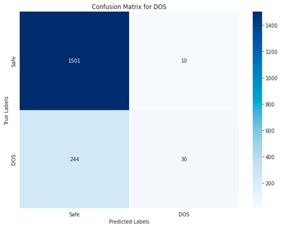
Figure 29.
Random Forest-RGB using Approach 1 for DOS class.
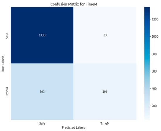
Figure 30.
Random Forest-RGB using Approach 1 for TimeM class.

Figure 31.
Random Forest-RGB using Approach 1 for TimeO class.
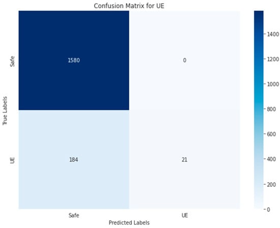
Figure 32.
Random Forest-RGB using Approach 1 for UE class.
As for the second approach, the multi-label classification was performed by using the test set that consisting of 1785 smart contract images. This test set was used for all the investigated algorithms except for RF and KNN; this is due to the limitation of the existing resources and the prolonged time required when 20% of the data set used was taken. Therefore, the percentage was reduced to 15% from each class, which represented a total of 1339 images (or contracts) for this test set. On the other hand, there was a difference in the test set in Approach 1 as compared to Approach 2 in which the four least classes were combined into one class (‘Others’), to enhance the balancing process. Figure 33 represents the distribution of vulnerabilities or classes within the test set where their distribution was as follows: ARTHM = 1295, RENT = 730, Others = 378, TimeM = 308, and LE = 246.
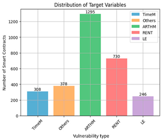
Figure 33.
Distribution of smart contract vulnerabilities in test set using Approach 2.
Figure 34, Figure 35, Figure 36, Figure 37 and Figure 38 show the five confusion matrices for the best multi-label classification algorithm using the second approach. The figure shows that many vulnerabilities were detected correctly. The presence of the ARTHM vulnerability was accurately detected in 1282 images, compared to the 1295 present in the original test set. However, for the ‘Others’ vulnerability class, only 104 grayscale images were correctly identified out of the 378 that contained this vulnerability. Conversely, 917 of these images were classified as not containing ‘Others’ but might contain other vulnerabilities. There were also 318 misclassified images, as there were 274 images that contained the ‘Others’ vulnerability that were not detected. This is likely due to the limitation of resources, as the number of decision trees used (‘n_estimators’) was set to only 100.
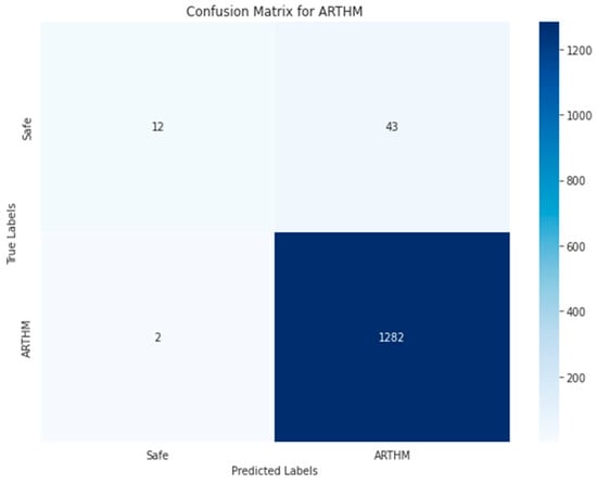
Figure 34.
Random Forest-GRAY using Approach 2 for ARTHM class.
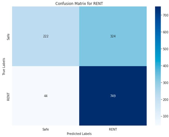
Figure 35.
Random Forest-GRAY using Approach 2 for RENT class.
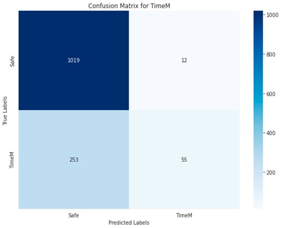
Figure 36.
Random Forest-GRAY using Approach 2 for TimeM class.
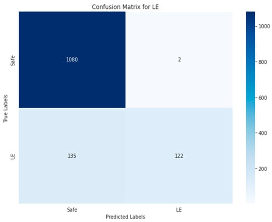
Figure 37.
Random Forest-GRAY using Approach 2 for LE class.
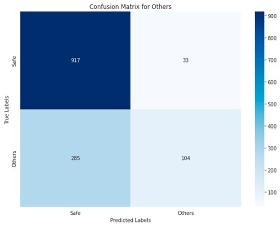
Figure 38.
Random Forest-GRAY using Approach 2 for the ‘Others’ class.
Finally, four of the classes with the least accuracy in previous approaches were combined into one ‘Others’ class for the third approach and the previous approach was combined into one ‘Others’ class. The distribution of these classes is represented in Figure 39. The ‘Others’ class contains 1761 smart contracts, and the remaining classes have the same distribution as their counterparts in the previous two approaches’ test groups. Accordingly, the total performance of all the algorithms mentioned previously in Section 3 was measured.
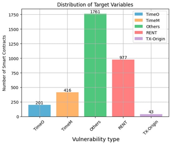
Figure 39.
Distribution of smart contracts vulnerabilities in test set using Approach 3.
The confusion matrices presented in Figure 40, Figure 41, Figure 42, Figure 43 and Figure 44 show how well the best multi-label classification algorithm (VGG19-RGB) in the third approach detects vulnerabilities in smart contracts. Each matrix details true positives, true negatives, false positives, and false negatives. Many vulnerabilities were correctly detected. Figure 44 shows that, for the ‘Others’ class, 1760 images (out of 1761) were correctly detected in TN, and 4 were correctly identified from the RGB images. There were only 21 misclassified images.
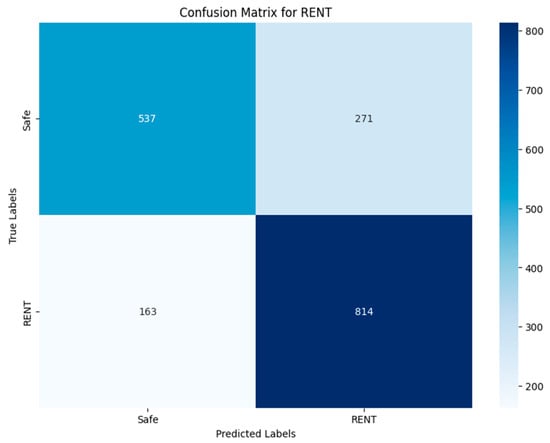
Figure 40.
VGG19-RGB using Approach 3 for RENT class.
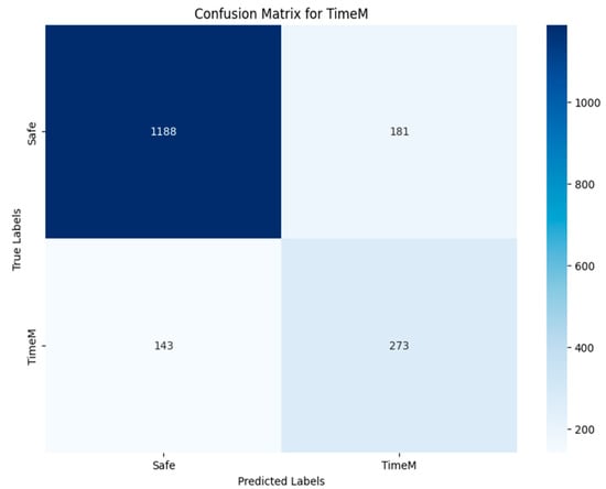
Figure 41.
VGG19-RGB using Approach 3 for TimeM class.

Figure 42.
VGG19-RGB using Approach 3 for TimeO class.
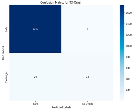
Figure 43.
VGG19-RGB using Approach 3 for TX-Origin class.
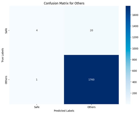
Figure 44.
VGG19-RGB using Approach 3 for the ‘Others’ class.
Figure 40 shows that 814 out of 977 images were detected in TN of the RENT class, with 537 images correctly classified as not containing the RENT vulnerability. The rest of the images were incorrectly predicted. In the case of identifying the TX-Origin vulnerability (Figure 43), 23 images were classified as containing it, out of the 43 images present in the original test set. A total of 22 were classified incorrectly, and the rest did not contain this vulnerability. Figure 41 and Figure 42 show that the prediction results for the TimeM and TimeO vulnerabilities in TN were 273 and 75, respectively, compared to 416 and 201 in the original test set. The VGG19-RGB matrices display a balanced distribution and a higher number of true positives.
4.3. Comparative Study
This study represents a significant contribution as the first of its kind to include binary and multi-label classification based on images of smart contract vulnerabilities. Table 4 compares the results of the multi-label classification algorithms used in this research with those from previous studies.

Table 4.
Comparison between this study and previous studies.
In the binary classification test for this study, the RF-RGB algorithm achieved the best performance among all algorithms. Due to the lack of prior research on binary classification targeting vulnerabilities in smart contracts, to the best of the author’s knowledge, and with respect to availability of the literature, there is no basis for comparison with other algorithms. Three approaches were applied to ensure the comprehensiveness of the results of this classification. The highest accuracy among all algorithms was for the VGG19-RGB algorithm, which achieved an accuracy rate of 89.14%; nevertheless, the accuracy rate alone cannot provide a trusted indicator of the algorithm’s efficiency. The F1-score must be involved as well. The use of both performance metrics can provide trusted insights into the algorithm’s performance. The highest accuracy value and F1-score were obtained for the VGG19-RGB algorithm in multi-label classification. Therefore, we will use its results for comparison with previous studies.
M. Rossini et al. [39] used four algorithms that specifically target the vulnerabilities in smart contracts and classify them in a multi-label classification. Their highest reported accuracy and F1-score were 73.53% and 83.81%, respectively, achieved using the ResNet1D algorithm. Our methodology using the VGG19-RGB algorithm significantly improves these performance metrics, achieving a 15.6% increase in accuracy and a 2.1% increase in the F1-score. Similarly, T. Hu et al. [22] utilized only the LSTM algorithm for multi-label classification, but their study reported only an F1-score of 77%. Our approach achieves a significant improvement of 8.6% in the F1-score.
The results of the performance metrics confirm our clear contribution to studying how effectively the proposed models perform in multi-label and binary classification. Based on the confusion matrices and benchmarks, VGG19 and RF are the best-performing algorithms, demonstrating their superiority in accurately classifying and detecting smart contract vulnerabilities. In addition, using the three approaches in multi-label classification demonstrates the accuracy of each algorithm and the extent to which the results differ in each of the algorithms used. It also emphasizes the importance of choosing the best algorithm based on the task’s requirements.
5. Conclusions
Smart contracts are of great importance in achieving the integrity of data and transactions in the blockchain. However, the vulnerabilities targeting smart contracts may limit their ability to be widespread. Therefore, this study aims to promote the use of smart contracts and preserve data and transactions by providing an enhanced methodology for the identification and classification of their possible vulnerabilities. Deep learning algorithms, namely ResNet50, VGG19, DenseNet201, KNN, and RF, were used to detect and classify vulnerabilities found in smart contracts by utilizing binary and multi-label classification techniques using two types of image formats: the RGB and grayscale images from two different datasets.
Interestingly, this research is the only and the first one that focused on binary classification in terms of studying and applying deep- and machine-learning algorithms to vulnerabilities targeting smart contracts. In that regard, the RF algorithm is considered to have the best performance in binary classification. Furthermore, we found that RGB images are better than grayscale images for binary classification tasks, with an accuracy of 86.66% and an F1 score of 86.66%. On the other hand, when moving to multi-label classification, RF using RGB images emerged as the standout algorithm in detecting vulnerabilities targeting smart contracts based on the results of the three multi-label classification approaches used in this study, achieving an impressive accuracy of 88.38%, F1-score of 78.26%, precision of 88.13%, and recall of 70.39%. The confusion matrices emphasized the result of VGG19-RGB’s balanced predictions, emphasizing its reliability in categorizing positive and negative instances. In the realm of multi-label classification under VGG19 with RGB images, approach three, which deletes categories with low precision, exhibited exceptional performance with perfect scores across various metrics, suggesting a high capacity to predict vulnerabilities with an accuracy of 89.14% and an F1-score of 85.87%.
The choice of the best algorithm ultimately depends on the specific requirements of the task. For binary classification of RGB images, RF is recommended, while VGG19-RGB excels in multi-label classification using the third approach when deleting classes with low accuracy. In the first two approaches, RF stands out with high performance, due to providing estimates of the importance of the selected features in classification to understand the impact of each feature and combining multiple trees predictions, which also positively affects performance. However, considerations such as interpretability, computational efficiency, and the nature of the task must guide the choice of the algorithm for effective vulnerability detection and classification. As for the best and optimal method that can be used to detect and classify vulnerabilities targeting smart contracts, deep learning algorithms proved to be more useful than instruction-based tools, because they are able to detect and classify vulnerabilities present in smart contracts more accurately and using one best algorithm. However, instruction-based tools do not fully detect vulnerabilities, and multiple tools must be used instead to detect the largest number of vulnerabilities present in contracts.
Future work will focus on investigating other deep learning algorithms and applying them to the proposed methodology with the aim of arriving at the best algorithm to increase the accuracy and efficiency in detecting and classifying vulnerabilities targeting smart contracts. We also propose to collect more real-world smart contracts which are correctly labeled, with the aim of using them for research and development purposes of blockchain systems in general and smart contracts in particular. This particularly opens future research into investigating more algorithms and lets current ones generalize better, leading to better performance in the real world.
Author Contributions
Conceptualization, R.M.B.-H. and A.S.S.; Methodology, R.M.B.-H. and A.S.S.; Software, L.A.-Y., R.M.B.-H. and A.S.S.; Supervision, R.M.B.-H. and A.S.S.; Validation, R.M.B.-H. and A.S.S.; Writing—original draft, L.A.-Y.; Writing—review & editing, R.M.B.-H. and A.S.S. All authors have read and agreed to the published version of the manuscript.
Funding
This research received no external funding.
Data Availability Statement
The RGB and Gray-Scale images dataset, and the source code of Binary Classification and Multi-Label Classification are available on the GitHub repository: https://github.com/lanaalyahya/Vulnerability-Classification-of-Ethereum-Smart-Contract-Using-Deep-Learning (Accessed on 20 August 2024).
Conflicts of Interest
The authors declare no conflict of interest.
References
- Wen, Y.; Lu, F.; Liu, Y.; Huang, X. Attacks and countermeasures on blockchains: A survey from layering perspective. Comput. Netw. 2021, 191, 107978. [Google Scholar] [CrossRef]
- Alizadeh, M.; Andersson, K.; Schelen, O. A survey of secure internet of things in relation to blockchain. J. Internet Serv. Inf. Secur. (JISIS) 2020, 10, 47–75. [Google Scholar]
- Farahani, B.; Firouzi, F.; Luecking, M. The convergence of IoT and distributed ledger technologies (DLT): Opportunities, challenges, and solutions. J. Netw. Comput. Appl. 2021, 177, 102936. [Google Scholar] [CrossRef]
- Uddin, M.A.; Stranieri, A.; Gondal, I.; Balasubramanian, V. A survey on the adoption of blockchain in iot: Challenges and solutions. Blockchain Res. Appl. 2021, 2, 100006. [Google Scholar] [CrossRef]
- Hewa, T.; Ylianttila, M.; Liyanage, M. Survey on blockchain based smart contracts: Applications, opportunities and challenges. J. Netw. Comput. Appl. 2021, 177, 102857. [Google Scholar] [CrossRef]
- Atzei, N.; Bartoletti, M.; Cimoli, T. A survey of attacks on ethereum smart contracts (sok). In Proceedings of the Principles of Security and Trust: 6th International Conference, POST 2017, Held as Part of the European Joint Conferences on Theory and Practice of Software, ETAPS 2017, Uppsala, Sweden, 22–29 April 2017; Proceedings 6. pp. 164–186. [Google Scholar]
- Vigliotti, M.G. What do we mean by smart contracts? Open challenges in smart contracts. Front. Blockchain 2021, 3, 553671. [Google Scholar] [CrossRef]
- Künnapas, K. From Bitcoin to Smart Contracts: Legal Revolution or Evolution from the Perspective of de lege ferenda? Future Law E Technol. 2016, 111–131. [Google Scholar] [CrossRef]
- Khan, S.N.; Loukil, F.; Ghedira-Guegan, C.; Benkhelifa, E.; Bani-Hani, A. Blockchain smart contracts: Applications, challenges, and future trends. Peer-Peer Netw. Appl. 2021, 14, 2901–2925. [Google Scholar] [CrossRef]
- Kushwaha, S.S.; Joshi, S.; Singh, D.; Kaur, M.; Lee, H.-N. Systematic review of security vulnerabilities in ethereum blockchain smart contract. IEEE Access 2022, 10, 6605–6621. [Google Scholar] [CrossRef]
- Tikhomirov, S.; Voskresenskaya, E.; Ivanitskiy, I.; Takhaviev, R.; Marchenko, E.; Alexandrov, Y. Smartcheck: Static analysis of ethereum smart contracts. In Proceedings of the 1st International Workshop on Emerging Trends in Software Engineering for Blockchain, Melbourne, Australia, 20 May 2023; pp. 9–16. [Google Scholar]
- Sayeed, S.; Marco-Gisbert, H.; Caira, T. Smart contract: Attacks and protections. IEEE Access 2020, 8, 24416–24427. [Google Scholar] [CrossRef]
- Zhou, H.; Milani Fard, A.; Makanju, A. The state of ethereum smart contracts security: Vulnerabilities, countermeasures, and tool support. J. Cybersecur. Priv. 2022, 2, 358–378. [Google Scholar] [CrossRef]
- Hu, B.; Zhang, Z.; Liu, J.; Liu, Y.; Yin, J.; Lu, R.; Lin, X. A comprehensive survey on smart contract construction and execution: Paradigms, tools, and systems. Patterns 2021, 2, 2. [Google Scholar] [CrossRef] [PubMed]
- Qian, P.; Liu, Z.; He, Q.; Huang, B.; Tian, D.; Wang, X. Smart contract vulnerability detection technique: A survey. arXiv 2022, arXiv:2209.05872. [Google Scholar]
- Perez, D.; Livshits, B. Smart contract vulnerabilities: Vulnerable does not imply exploited. In Proceedings of the 30th USENIX Security Symposium (USENIX Security 21), Vancouver, BC, USA, 11–13 August 2021; pp. 1325–1341. [Google Scholar]
- Rouhani, S.; Deters, R. Security, performance, and applications of smart contracts: A systematic survey. IEEE Access 2019, 7, 50759–50779. [Google Scholar] [CrossRef]
- Zaidi, S.Y.A.; Shah, M.A.; Khattak, H.A.; Maple, C.; Rauf, H.T.; El-Sherbeeny, A.M.; El-Meligy, M.A. An attribute-based access control for IoT using blockchain and smart contracts. Sustainability 2021, 13, 10556. [Google Scholar] [CrossRef]
- Wang, S.; Ouyang, L.; Yuan, Y.; Ni, X.; Han, X.; Wang, F.-Y. Blockchain-enabled smart contracts: Architecture, applications, and future trends. IEEE Trans. Syst. Man Cybern. Syst. 2019, 49, 2266–2277. [Google Scholar] [CrossRef]
- Yashavant, C.S.; Kumar, S.; Karkare, A. Scrawld: A dataset of real world ethereum smart contracts labelled with vulnerabilities. arXiv 2022, arXiv:2202.11409. [Google Scholar]
- Feist, J.; Grieco, G.; Groce, A. Slither: A static analysis framework for smart contracts. In Proceedings of the 2019 IEEE/ACM 2nd International Workshop on Emerging Trends in Software Engineering for Blockchain (WETSEB), Montreal, QC, USA, 27 May 2019; pp. 8–15. [Google Scholar]
- Hu, T.; Liu, X.; Chen, T.; Zhang, X.; Huang, X.; Niu, W.; Lu, J.; Zhou, K.; Liu, Y. Transaction-based classification and detection approach for Ethereum smart contract. Inf. Process. Manag. 2021, 58, 102462. [Google Scholar] [CrossRef]
- Smart Contract Weakness Classification (SWC) Registry, Integer Overflow and Underflow. 2020. Available online: https://swcregistry.io/docs/SWC-101/ (accessed on 12 August 2024).
- Khor, J.; Masama, M.A.; Sidorov, M.; Leong, W.; Lim, J. An improved gas efficient library for securing IoT smart contracts against arithmetic vulnerabilities. In Proceedings of the 2020 9th International Conference on Software and Computer Applications, Langkawi, Malaysia, 18–21 February 2020; pp. 326–330. [Google Scholar]
- Smart Contract Weakness Classification (SWC) Registry, DoS with Failed Call. 2020. Available online: https://swcregistry.io/docs/SWC-113/ (accessed on 12 August 2024).
- Smart Contract Weakness Classification (SWC) Registry, DoS with Block Gas Limit. 2020. Available online: https://swcregistry.io/docs/SWC-128 (accessed on 12 August 2024).
- Durieux, T.; Ferreira, J.F.; Abreu, R.; Cruz, P. Empirical review of automated analysis tools on 47,587 ethereum smart contracts. In Proceedings of the ACM/IEEE 42nd International Conference on Software Engineering, Seoul, Republic of Korea, 27 June 2020; pp. 530–541. [Google Scholar]
- Smart Contract Weakness Classification (SWC) Registry, Reentrancy. 2020. Available online: https://swcregistry.io/docs/SWC-107/ (accessed on 12 August 2024).
- Smart Contract Weakness Classification (SWC) Registry, Block Values as a Proxy for Time. 2020. Available online: https://swcregistry.io/docs/SWC-116/ (accessed on 12 August 2024).
- Smart Contract Weakness Classification (SWC) Registry, Transaction Order Dependence. 2020. Available online: https://swcregistry.io/docs/SWC-114/ (accessed on 12 August 2024).
- Smart Contract Weakness Classification (SWC) Registry, Unchecked Call Return Value. 2020. Available online: https://swcregistry.io/docs/SWC-104/ (accessed on 12 August 2024).
- Smart Contract Weakness Classification (SWC) Registry, Authorization through tx.origin. 2020. Available online: https://swcregistry.io/docs/SWC-115/ (accessed on 12 August 2024).
- Zhao, H.; Tan, J. A critical-path-based vulnerability detection method for tx. origin dependency of smart contract. In Proceedings of International Conference on Smart Computing and Communication, New York, NY, USA, 18–20 November 2022; pp. 393–402. [Google Scholar]
- Wu, C.; Xiong, J.; Xiong, H.; Zhao, Y.; Yi, W. A review on recent progress of smart contract in blockchain. IEEE Access 2022, 10, 50839–50863. [Google Scholar] [CrossRef]
- Soud, M.; Qasse, I.; Liebel, G.; Hamdaqa, M. Automesc: Automatic framework for mining and classifying ethereum smart contract vulnerabilities and their fixes. In Proceedings of the 2023 49th Euromicro Conference on Software Engineering and Advanced Applications (SEAA), Durres, Albania, 6–8 September 2023; pp. 410–417. [Google Scholar]
- Aldweesh, A.; Alharby, M.; Mehrnezhad, M.; Van Moorsel, A. OpBench: A CPU performance benchmark for Ethereum smart contract operation code. In Proceedings of the 2019 IEEE International Conference on Blockchain (Blockchain), Atlanta, GA, USA, 4–17 July 2019; pp. 274–281. [Google Scholar]
- Jiang, Z.; Chen, K.; Wen, H.; Zheng, Z. Applying blockchain-based method to smart contract classification for CPS applications. Digit. Commun. Netw. 2022, 8, 964–975. [Google Scholar] [CrossRef]
- Khodadadi, M.; Tahmoresnezhad, J. Hymo: Vulnerability detection in smart contracts using a novel multi-modal hybrid model. arXiv 2023, arXiv:2304.13103. [Google Scholar]
- Rossini, M.; Zichichi, M.; Ferretti, S. Smart contracts vulnerability classification through deep learning. In Proceedings of the 20th ACM Conference on Embedded Networked Sensor Systems, Boston, MA, USA, 6–9 November 2022; pp. 1229–1230. [Google Scholar]
- Chavhan Sujeet Yashavant, Saurabh Kumar, and Amey Karkare. ScrawlD Dataset. Available online: https://github.com/sujeetc/ScrawlD (accessed on 12 August 2024).
- Rossini, M. Slither Audited Smart Contracts Dataset. Available online: https://huggingface.co/datasets/mwritescode/slither-audited-smart-contracts/viewer/all-multilabel/train (accessed on 12 August 2024).
- Ethereum, Etherscan. 2015. Available online: https://etherscan.io/apis (accessed on 12 August 2024).
- Whang, S.E.; Roh, Y.; Song, H.; Lee, J.-G. Data collection and quality challenges in deep learning: A data-centric ai perspective. VLDB J. 2023, 32, 791–813. [Google Scholar] [CrossRef]
- Alon, U.; Zilberstein, M.; Levy, O.; Yahav, E. code2vec: Learning distributed representations of code. Proc. ACM Program. Lang. 2019, 3, 1–29. [Google Scholar] [CrossRef]
- Vasilev, I.; Slater, D.; Spacagna, G.; Roelants, P.; Zocca, V. Python Deep Learning: Exploring Deep Learning Techniques and Neural Network Architectures with Pytorch, Keras, and TensorFlow; Packt Publishing Ltd.: Birmingham, UK, 2019. [Google Scholar]
- Sarkar, D.; Bali, R.; Ghosh, T. Hands-On Transfer Learning with Python: Implement Advanced Deep Learning and Neural Network Models Using TensorFlow and Keras; Packt Publishing Ltd.: Birmingham, UK, 2018. [Google Scholar]
- Jeremy Andrews, Google Colab. 2017. Available online: https://colab.research.google.com/ (accessed on 12 August 2024).
- Reghunath, A.; Nair, S.V.; Shah, J. Deep learning based customized model for features extraction. In Proceedings of the 2019 International Conference on Communication and Electronics Systems (ICCES), Coimbatore, India, 17–19 July 2019; pp. 1406–1411. [Google Scholar]
- Gergerli, B.; Çelebi, F.V.; Rahebi, J.; Şen, B. An Approach Using in Communication Network Apply in Healthcare System Based on the Deep Learning Autoencoder Classification Optimization Metaheuristic Method. Wirel. Pers. Commun. 2023, pp. 1–24. [CrossRef]
- Mascarenhas, S.; Agarwal, M. A comparison between VGG16, VGG19 and ResNet50 architecture frameworks for Image Classification. In Proceedings of the 2021 International Conference on Disruptive Technologies for Multi-Disciplinary Research and Applications (CENTCON), Bengaluru, India, 19–21 November 2021; pp. 96–99. [Google Scholar]
- Meghana, Resnet50. 2023. Available online: https://datagen.tech/guides/computer-vision/resnet-50/ (accessed on 12 August 2024).
- Sanghvi, H.A.; Patel, R.H.; Agarwal, A.; Gupta, S.; Sawhney, V.; Pandya, A.S. A deep learning approach for classification of COVID and pneumonia using DenseNet-201. Int. J. Imaging Syst. Technol. 2023, 33, 18–38. [Google Scholar] [CrossRef]
- Jaiswal, A.; Gianchandani, N.; Singh, D.; Kumar, V.; Kaur, M. Classification of the COVID-19 infected patients using DenseNet201 based deep transfer learning. J. Biomol. Struct. Dyn. 2021, 39, 5682–5689. [Google Scholar] [CrossRef]
- Kong, Y.; Yu, T. A deep neural network model using random forest to extract feature representation for gene expression data classification. Sci. Rep. 2018, 8, 16477. [Google Scholar] [CrossRef]
- Ham, J.; Chen, Y.; Crawford, M.M.; Ghosh, J. Investigation of the random forest framework for classification of hyperspectral data. IEEE Trans. Geosci. Remote Sens. 2005, 43, 492–501. [Google Scholar] [CrossRef]
- Fuadah, Y.N.; Pramudito, M.A.; Lim, K.M. An optimal approach for heart sound classification using grid search in hyperparameter optimization of machine learning. Bioengineering 2022, 10, 45. [Google Scholar] [CrossRef]
- An, J.; Ying, L.; Zhu, Y. Why resampling outperforms reweighting for correcting sampling bias with stochastic gradients. arXiv 2020, arXiv:2009.13447. [Google Scholar]
- Heydarian, M.; Doyle, T.E.; Samavi, R. MLCM: Multi-label confusion matrix. IEEE Access 2022, 10, 19083–19095. [Google Scholar] [CrossRef]
- Grandini, M.; Bagli, E.; Visani, G. Metrics for multi-class classification: An overview. arXiv 2020, arXiv:2008.05756. [Google Scholar]
- Ganda, D.; Buch, R. A survey on multi label classification. Recent Trends Program. Lang. 2018, 5, 19–23. [Google Scholar]
Disclaimer/Publisher’s Note: The statements, opinions and data contained in all publications are solely those of the individual author(s) and contributor(s) and not of MDPI and/or the editor(s). MDPI and/or the editor(s) disclaim responsibility for any injury to people or property resulting from any ideas, methods, instructions or products referred to in the content. |
© 2024 by the authors. Licensee MDPI, Basel, Switzerland. This article is an open access article distributed under the terms and conditions of the Creative Commons Attribution (CC BY) license (https://creativecommons.org/licenses/by/4.0/).