A Novel Traffic Classification Approach by Employing Deep Learning on Software-Defined Networking

Abstract

The ever-increasing diversity of Internet applications and the rapid evolution of network infrastructure due to emerging technologies have made network management more challenging. Effective traffic classification is critical for efficiently managing network resources and aligning with service quality and security demands. The centralized controller of software-defined networking provides a comprehensive network view, simplifying traffic analysis and offering direct programmability features. When combined with deep learning techniques, these characteristics enable the incorporation of intelligence into networks, leading to optimization and improved network management and maintenance. Therefore, this research aims to develop a model for traffic classification by application types and network attacks using deep learning techniques to enhance the quality of service and security in software-defined networking. The SEMMA method is employed to deploy the model, and the classifiers are trained with four algorithms, namely LSTM, BiLSTM, GRU, and BiGRU, using selected features from two public datasets. These results underscore the remarkable effectiveness of the GRU model in traffic classification. Hence, the outcomes achieved in this research surpass state-of-the-art methods and showcase the effectiveness of a deep learning model within a traffic classification in an SDN environment.

1. Introduction

In an increasingly digital world characterized by the rapid proliferation of smart devices and emerging technologies, data traffic is experiencing exponential growth. Consequently, network infrastructures are becoming progressively more diverse and complex to efficiently handle traffic distribution and the management of numerous devices [1]. A typical production network comprises multiple devices, operates protocols, and supports various applications. The heterogeneity of network infrastructures presents numerous challenges regarding effective organization, resource optimization, and management [2]. The introduction of intelligence into networks has been proposed to address these challenges [3]. One approach suggested several years ago involves implementing a knowledge plane (KP) that incorporates machine learning (ML) and deep learning (DL) techniques [4]. Likewise, recent advances in networking include network programmability facilitated by software-defined networking (SDN) [5]. Thus, Internet Service Providers (ISPs) and network administrators must adjust to these transformations by implementing the right tools and methodologies to guarantee effective network management.

SDN is an emerging and dynamic architectural approach that separates the control plane from the data plane. This technology is particularly well-suited to the constantly changing nature of modern applications. The centralized controller within SDN provides a comprehensive network view, enabling the monitoring, configuration, and control switches to manage the traffic flows [6]. The SDN controller collects information about network flows and offers real-time programmability, making it conducive to integrating ML models. This integration can infuse intelligence into the SDN controller, enabling it to perform tasks such as data analysis, traffic classification, resource management, security, and general network services [7]. However, while the controller enables efficient flow control, it cannot achieve distributed end-to-end QoS management and control attacks due to the lack of control of end users. Hence, incorporating ML techniques into SDN has garnered significant interest as it offers innovative data-driven approaches to tackle conventional network challenges.

Traffic classification is a complex endeavor that entails categorizing network traffic into specific classes, serving various objectives, including network management, service measurement, and network monitoring. Additionally, it plays a crucial role in enabling efficient resource allocation and configuring access controls, quality of service (QoS), and other network security parameters. Commonly utilized traffic classification methods include the port-based method [8], statistical approach [9] and Deep Packet Inspection (DPI) [10,11]. Nevertheless, these traditional techniques have become less effective, with most applications now operating on dynamic ports and network traffic encryption. Hence, there is a need to develop a novel classification technique that is better suited to the current operational conditions.

Artificial Intelligence (AI) has become essential for analyzing and sorting network traffic [12]. This technique collects data and applies machine learning algorithms to classify and identify various types of network traffic. It observes patterns and features transmitted within network packets, such as their size, duration, and frequency. Analyzing the contextual information associated with the packets allows for categorizing traffic into specific groups, including encrypted traffic [13,14]. Therefore, software-defined networking (SDN) and machine learning techniques represent a precise and efficient classification method [15]. Recently, the integration of SDN and the use of Deep Learning (DL) methods have provided viable alternatives that have improved the classification of traffic flows by application type [16,17]. As a result, this enhances the user experience and optimizes network performance by assigning priority based on quality of service (QoS) and network security requirements.

Despite the numerous studies on traffic classification using deep learning (DL) in software-defined networking (SDN) environments, challenges still need to be addressed. These include classifying new traffic categories, optimizing classification approaches, and fine-tuning hyperparameter settings. DL is a practical approach that offers various algorithms that have proven highly effective in traffic classification tasks. Therefore, this research aims to design a traffic classification model using DL algorithms, explicitly focusing on classifying traffic flows by application type and network attacks. The main contributions of this work can be summarized as follows:

• We have developed four classifiers with DL algorithms to evaluate which offers better results based on two open datasets. Specifically, we used the Gated Recurrent Unit (GRU), Bidirectional Gated Recurrent Unit (BiGRU), Long Short-Term Memory(LSTM), and Bidirectional Long Short-Term Memory (BiLSTM) algorithms. In related work, we observed a lack of classifiers that specifically use GRU, BiGRU, and BiLSTM algorithms for multiclass traffic classification in SDNs.
• The classifiers aim to improve the SDN performance and security by using the traffic flow to identify application types and attacks in five classes: Multimedia, VoIP, Instant message, File transfer, and Attacks. One of the main innovations of our approach lies in integrating attack detection into the classification process, thus addressing a gap identified in the related work. The experiments demonstrate the accuracy of detecting different application types and attacks, such as Denial of Service (DoS), Distributed Denial of Service (DDoS), Brute-force-attack, Exploitation (R2L), Web_attack, Botnet, and Probe.
• The selection of features based on analysis of the SDN controllers and sequence length enabled an appropriate generalization of deep learning models. This choice facilitates implementing classifiers in SDN with any controller because northern interfaces can obtain the selected features, thus reducing the complexity of model training, improving traffic classification accuracy, and decreasing the associated computational cost.

The paper is structured as follows: Section 2 discusses related work, Section 3 presents the proposed methodology, Section 4 shows the results and discussion, and finally, Section 5 explains the conclusions and lines of future work.

2. Related Work

In recent times, researchers have been attempting to apply statistical methods for DL traffic classification. These methods utilize payload-independent parameters such as packet length, inter-arrival time, and flow duration. This section will analyze and discuss previous work based on DL techniques in SDN for traffic classification. We have summarized the outcomes of these studies in

Table 1. Deep learning-based traffic classification in SDN.

Ref.	Classification Objective	Model Input	Model Output	Accuracy
[18]	QoS-aware	Automatic by algorithm	15 applications	MLP: 97.14% SAE: 99.14% CNN: 99.30%
[19]	QoS-aware	Automatic by algorithm	10 classes	SAE: >90.00%
[20]	Application-aware	Automatic by algorithm	8 applications	ML-LSTM: 97.14%
[21]	Application-aware	4 features	6 applications	CNN: 93.35% MLP: 93.21% SAE: 93.13%
[22]	QoS-aware	23 features	3 classes	CNN: 96.00% DNN: 94.00%
[23]	Application-aware	Flow features selected by autoencoders	24 applications	CNN+autoencoder: 97.42% CNN: 96.03% DNN: 94.36%
[24]	Application-aware	Automatic by algorithm	15 applications	GAN: 93.18% CNN: 93.30%
[25]	Application-aware	Automatic by algorithm	5 classes	CNN: 98.85% LSTM: 99.22% SAE: 98.74%
[26]	QoS-aware	Automatic by algorithm	20 applications	MLP, CNN and SAE: >90.00%
[27]	QoS-aware	20 features	8 classes	ResNet: 97.24%
[28]	QoS-aware	6 features	6 classes	VAE: 89.00%

.

The first study mentioned in Table 1 is by Wang et al. [18]. They introduced an approach called SDN-HGW, which enhances the management of distributed smart home networks. The approach supports the core network controller and extends control to the access network, allowing for more effective end-to-end network management. This framework is of great importance in smart home networks. It enables awareness of distributed applications using data traffic classification within the network. To achieve this, the authors developed encrypted classifiers called DataNets. These classifiers are designed using three deep learning algorithms: Multilayer Perceptron (MLP), Stacked Autoencoder (SAE), and Convolutional Neural Networks (CNNs). The classifiers are trained using an open dataset that includes data from 15 applications, encompassing over 200,000 encrypted data samples. The study’s results demonstrate the applicability of these classifiers in a smart home SDN environment, enabling distributed application awareness.

Zhang et al. [19] introduced a novel classification approach, as outlined in their research. This approach relies on a hybrid deep neural network for application classification. Notably, it automatically derives flow features from the Stacked Autoencoder (SAE) algorithm, eliminating the need for manual feature selection. In conjunction with this, a centralized SDN controller efficiently acquires and processes extensive network traffic, leveraging its substantial computing capabilities. The findings from their study indicate that this novel classification method outperforms the traditional Support Vector Machine (SVM)-based approach in terms of accuracy.

Lim et al. [20] presented a schema for traffic classification in SDN using DL models. They prepared a dataset by preprocessing network traffic flows. They developed two DL classifiers: the Multi-layer Long Short-term Memory (ML-LSTM) model and a combination of a CNN and single-layer LSTM. The hyperparameters of the models were adjusted using a fitting procedure. As indicated by the F1 score, performance analysis revealed the ML-LSTM model’s superiority in network packet classification.

Chang et al. [21] introduced a novel application-aware traffic classification model within an SDN testbed for online and offline usage. This model is integrated into the SDN controller and uses three DL algorithms: MPL, CNN, and SAE. An open dataset of samples from the seven most popular applications was used to train the model. The results showed that the model achieved an impressive accuracy of over 93.00% during offline training and maintained a notable 87.00% accuracy during online testing.

Abdulrazzaq and Demirci [22] have developed an engineering system that manages traffic in software-defined networking (SDN) to enhance bandwidth allocation for various applications. Their system is based on a classifier built using deep neural network (DNN) and 1D-CNN algorithms. The Synthetic Minority Over-Sampling Technique (SMOTE) addresses imbalanced class distribution within the dataset. The main goal of this system is to improve service quality by assigning different priority queues based on the classification of traffic flows that originate from other applications. Their research shows that DNN and 1D CNN algorithms offer higher accuracy when dealing with traffic data captured within 5 s and 10 s timeouts.

Chiu et al. [23] introduced a system known as the Convolutional Autoencoder Packet Classifier (CAPC), designed to promptly categorize incoming packets in both fine-grained and coarse-grained manners, distinguishing individual applications and broader categories, respectively, using DL. CAPC is a packet-based deep learning model comprising a 1D convolutional neural network and an autoencoder, enabling it to effectively manage dynamic ports, encrypted traffic, and even group similar applications. The classifier is evaluated using a privately collected traffic dataset and a publicly available VPN dataset, highlighting its exceptional performance. CAPC exhibits an accuracy exceeding 97.00% when classifying service traffic types on the public dataset containing 24 services.

Wang et al. [24] developed a semi-supervised traffic classification technique in SDN called ByteS-GAN, which utilizes Generative Adversarial Networks (GAN). ByteS-GAN was created to achieve high accuracy, even with limited labeled samples and many unlabeled data. The approach involved modifying the structure and loss function of the traditional GAN discriminator network to enable fine-grained traffic classification. The research results show that ByteS-GAN significantly improves the classifier’s performance, outperforming supervised methods such as CNN.

In their work, Wu et al. [25] have presented a framework that uses a deep learning algorithm to classify encrypted network traffic. The framework comprises three modules, with the first module responsible for preprocessing the network flows, the second module focusing on training the classifier, and the third module dealing with testing the CNN model. According to their findings, this encrypted network traffic classification framework performs effectively and uses low resources.

Setiawan et al. [26] introduced a framework to enhance the security of the SDN controller while improving the management of smart home networks. This framework, named SDN Home GateWay for Congestion (SDNHGC), is based on DL algorithms. SDNHGC conducts real-time traffic analysis to facilitate the regulation of network capacity and resource allocation. The classifier within the framework was trained and tested using samples from 20 applications sourced from an open database, employing algorithms such as SAE, MLP, and CNN. The results demonstrate that this approach achieves a level of accuracy superior to other existing solutions.

Anh et al. [27] sought to tackle the challenge of interpretability in DL-based traffic classification by introducing an explanatory method incorporating a genetic algorithm. They designed a traffic classifier based on the ResNet model and employed the genetic algorithm to create optimal feature selection masks. This innovative approach yielded an impressive accuracy rate of around 97.24%. Notably, by quantifying the significance of individual features and calculating their dominance rate, the authors provided valuable insights into how the classifier operates for various Internet services, shedding light on its underlying mechanisms.

Jang et al. [28] tackled the challenge of traffic classification within SDN environments by introducing an innovative approach that leverages a variational autoencoder (VAE). Their objective was to effectively categorize different classes of Internet services and ensure the quality of service. To achieve this, the VAE was trained using six statistical features, enabling the extraction of latent feature distributions for flows within each service class. The classification of query traffic was accomplished by comparing its latent feature distribution with the previously learned distributions. The experimental results demonstrated the efficacy of this method, with an average accuracy of 89.00%, surpassing the performance of conventional statistics-based and machine learning-based approaches.

In the literature review, the authors propose traffic classification models with DL techniques, which were analyzed based on accuracy, number of input features, and number of classes identified in the model output. Although the models demonstrate good accuracy, problems such as multiclass imbalance, training time, computational cost, and availability of the training dataset persist. In addition, with the exponential growth of applications and the constant change in network attack signatures, another challenge arises in network traffic classification, known as concept drift. Variations in the environment and data distribution occur due to temporal location fluctuations.

Identifying all applications and all network attacks is a complex and impractical task. Therefore, the present research proposes developing a DL-based classifier that identifies applications and the most common network attacks into classes based on specific traffic flow characteristics. With this proposal, different applications and attacks can be grouped into classes. This classification of application and attack traffic flows is more efficient than classifying them individually, facilitating assigning QoS policies or restrictions to the network traffic.

3. Materials and Methods

This section details the SEMMA methodology used to develop the research [29]. Each of the SEMMA stages must be performed sequentially to generate a precise traffic classifier: sampling, exploration, modification, modeling, and assessment. It is important to note that the structure of this methodology aligns with our research objective, which is to efficiently build a traffic classification model in SDN with deep learning techniques. Figure 1 illustrates the flowchart of the improved SEMMA data science methodology.

3.1. Sample

In this phase, the initial dataset is selected. At this point, the researcher can choose to work with the entire dataset, or they can choose to select a representative sample of the original dataset. The data came from two public datasets, InSDN [30] and ISCX-VPN-NoVPN [31]. The InSDN dataset is developed over a specific SDN network to generate regular and attack traffic, essential for evaluating performance or creating new intrusion detection systems. The logs for each traffic type are in CSV files, which are approximately 1.88 GB and 3.58 GB in size, respectively. The ISCX-VPN-NoVPN dataset has different kinds of application traffic, allowing other aspects and scenarios to be addressed. Its files are in PCAP format, indicating the data is unprocessed. The data are divided into five zip files; three files are nonVPN, and two are VPN, totaling 28.00 GB of raw data.

The network flows from the PCAP files obtained from two datasets were extracted using the CICFlowMeter tool [31]. The tool, developed by the Canadian Institute for Cybersecurity (CIC) at the University of New Brunswick, Canada, is written in Java. It can extract time-based features from network flows, which are essential for calculating time-related statistics. The generated flows are computed bidirectionally. In the study conducted by [32], the tool’s output was configured with a flow timeout of 15 s, extracting 83 features in CSV file format. The study [33] also used the time-base features of the InSDN dataset. Based on this approach,

Table 2. Preprocessed dataset.

Dataset	Content	Samples
ICSX VPN–nonVPN	AIM chat	1033
	BitTorrent	777
	Email Client	6976
	Facebook Audio	62,544
	Facebook Chat	2285
	Facebook Video	1226
	FTPS	2045
	Gmail Chat	1053
	Hangouts Audio	72,397
	Hangouts Chat	4033
	Hangouts Video	2882
	ICQ	1131
	Netflix	2084
	SCP	9546
	SFTP	449
	Skype Audio	27,756
	Skype Chat	6703
	Skype File	42,640
	Skype Video	1594
	Spotify	1498
	Vimeo	1752
	VoIP Buster	6217
	YouTube	2962
InSDN	DDoS	121,942
	DoS	53,616
	Probe	98,129
	Brute-force-attack	1405
	Exploitation (R2L)	17
	Web_attack	192
	Botnet	164

presents the details of the datasets after processing the PCAP files with a flow timeout of 15 s.

3.2. Explore

The dataset for this research was organized into five traffic classes, created by combining the two datasets detailed in Table 2. The ICSX VPN–nonVPN dataset excluded applications such as BitTorrent, Email Client, and Spotify since they could not be assigned to any of the five classes or needed sufficient samples. On the other hand, in the InSDN dataset, attacks with limited samples, such as Botnet, Web_attack, and Exploitation (R2L), were not discarded. Ultimately, a random and equitable selection process of examples was conducted for applications and attacks to balance the five classes. The result of this sample selection process is presented in

Table 3. Dataset samples selection.

Class	Content	Total Samples	Selected Samples
Multimedia	Facebook Video, Hangouts Video, Skype Video, Netflix, Vimeo, YouTube	12,500	10,000
VoIP	Facebook Audio, Hangouts Audio, Skype Audio, VoIP Buster	168,914	10,000
Instant message	AIM Chat, Facebook Chat, Gmail Chat, Hangouts Chat, ICQ, Skype Chat	16,238	10,000
File transfer	FTPS, SCP, SFTP, Skype File	54,680	10,000
Attack	DDoS, DoS, Probe, Brute-force-attack, Exploitation (R2L), Web_attack, Botnet	275,515	10,000

. In addition,

Table 4. List of extracted features.

No.	Feature Name	No.	Feature Name	No.	Feature Name
1	Flow ID	29	Fwd IAT Std	57	ECE Flag Cnt
2	Src IP	30	Fwd IAT Max	58	Down/Up Ratio
3	Src Port	31	Fwd IAT Min	59	Pkt Size Avg
4	Dst IP	32	Bwd IAT Tot	60	Fwd Seg Size Avg
5	Dst Port	33	Bwd IAT Mean	61	Bwd Seg Size Avg
6	Protocol	34	Bwd IAT Std	62	Fwd Byts/b Avg
7	Timestamp	35	Bwd IAT Max	63	Fwd Pkts/b Avg
8	Flow Duration	36	Bwd IAT Min	64	Fwd Blk Rate Avg
9	Tot Fwd Pkts	37	Fwd PSH Flags	65	Bwd Byts/b Avg
10	Tot Bwd Pkts	38	Bwd PSH Flags	66	Bwd Pkts/b Avg
11	TotLen Fwd Pkts	39	Fwd URG Flags	67	Bwd Blk Rate Avg
12	TotLen Bwd Pkts	40	Bwd URG Flags	68	Subflow Fwd Pkts
13	Fwd Pkt Len Max	41	Fwd Header Len	69	Subflow Fwd Byts
14	Fwd Pkt Len Min	42	Bwd Header Len	70	Subflow Bwd Pkts
15	Fwd Pkt Len Mean	43	Fwd Pkts/s	71	Subflow Bwd Byts
16	Fwd Pkt Len Std	44	Bwd Pkts/s	72	Init Fwd Win Byts
17	Bwd Pkt Len Max	45	Pkt Len Min	73	Init Bwd Win Byts
18	Bwd Pkt Len Min	46	Pkt Len Max	74	Fwd Act Data Pkts
19	Bwd Pkt Len Mean	47	Pkt Len Mean	75	Fwd Seg Size Min
20	Bwd Pkt Len Std	48	Pkt Len Std	76	Active Mean
21	Flow Byts/s	49	Pkt Len Var	77	Active Std
22	Flow Pkts/s	50	FIN Flag Cnt	78	Active Max
23	Flow IAT Mean	51	SYN Flag Cnt	79	Active Min
24	Flow IAT Std	52	RST Flag Cnt	80	Idle Mean
25	Flow IAT Max	53	PSH Flag Cnt	81	Idle Std
26	Flow IAT Min	54	ACK Flag Cnt	82	Idle Max
27	Fwd IAT Tot	55	URG Flag Cnt	83	Idle Min
28	Fwd IAT Mean	56	CWE Flag Count	84	Label

shows all the features of the dataset.

3.3. Modify

This phase involves modifying the dataset, including data cleaning, variable transformation, and feature selection. Therefore, the following section will provide a detailed overview of the process.

3.3.1. Data Cleaning

Data cleaning is a crucial step in data analysis, ensuring the data’s quality and integrity. Anomalies such as missing values and outliers can exist within datasets, and addressing them helps improve the analysis’s reliability. According to Garcia et al. [34], there are three types of missing values: Missing Completely At Random (MCAR), where values have a high likelihood of missing in the dataset across various instances and attributes; Missing At Random (MAR), where missing values are observed in any of the attributes; and Not Missing At Random (NMAR), where values are absent because they depend on another value that is also missing. During data inspection and visualization, we encountered four MAR-type missing values for the “Flow Byts/s” feature. The present work utilized Python as the primary programming language to address the issue by employing the Pandas library’s mean() and fillna() functions. These functions allowed us to replace the null values in the dataset with the corresponding means.

In a dataset, there are outliers, that is, data points that deviate from others, either in terms of the data’s location, distinct behavior, or uncommon values within the same feature. As indicated by Wang et al. [35], there are various methods for detecting these values, including those based on statistical techniques, distance between observations, density, clustering, and machine learning. We identified six records with infinite values and subsequently removed them during data inspection.

3.3.2. Label Encoding

Transformation of the target variable labels from letters to integers was carried out to enhance the distribution of the target variables and align with model requirements. This numerical transformation allowed the models to operate more effectively using numerical values instead of letter categories. This process employed two libraries, Keras’ to_categorical, and Scikit-learn LabelEncoder, working in tandem to take categorical labels and prepare them for use in deep learning models. First, a LabelEncoder was created to map categorical labels to numerical values. Labels such as “multimedia”, “voip”, “instantmessage”, “filetransfer”, and “attack”, were assigned to each traffic class are allocated unique numerical values. Subsequently, one-hot encoding was applied using the to_categorical function. This transformation converts numerical values into binary vectors, where each label is represented by a vector with a single active bit set to 1 and the remainder set to 0. Ultimately, an encoded one-hot matrix was obtained and served as target labels in machine learning models. It is important to emphasize that this process is crucial for enabling models to understand and classify categories in classification problems effectively.

3.3.3. Data Scaling

Standardization is a process that transforms the features of a dataset in such a way that they have a uniform scale and follow a standard normal distribution with a mean of zero and a standard deviation of one. Equation (1) represents the mathematical formulation of the z-score scaling standardization transformation, which was used in this process. Normalization is a fundamental technique in developing deep learning models, as it eliminates differences in feature scales, ensuring that all features have an equal impact and, thereby, facilitating feature comparison and interpretation. We employed the StandardScaler library from sci-kit-learn to perform the feature scaling transformation on the dataset.

$$\begin{array}{cc}\hfill Z& =\frac{(xi-mean(x\left)\right)}{stdev\left(x\right)}\hfill \end{array}$$

(1)

3.3.4. Feature Selection

This stage aims to select the most relevant features of a dataset to train a DL model. This is done to improve the model’s accuracy, reduce the data’s dimensionality, and facilitate the interpretation of the results. To this end, a thorough data analysis and feature engineering techniques are applied. Initially, it is essential to understand the data and, from that understanding, to infer the information that can be derived from them. As a result, we identified 12 features with constant values across all samples in the dataset: “Fwd PSH Flags”, “Fwd URG Flags”, “CWE Flag Count”, “ECE Flag Cnt”, “Fwd Byts/b Avg”, “Fwd Pkts/b Avg”, “Fwd Blk Rate Avg”, “Bwd Byts/b Avg”, “Bwd Pkts/b Avg”, “Bwd Blk Rate Avg”, “Init Fwd Win Byts”, and “Fwd Seg Size Min ”. Consequently, we discarded these features as they did not provide meaningful information for classifier training.

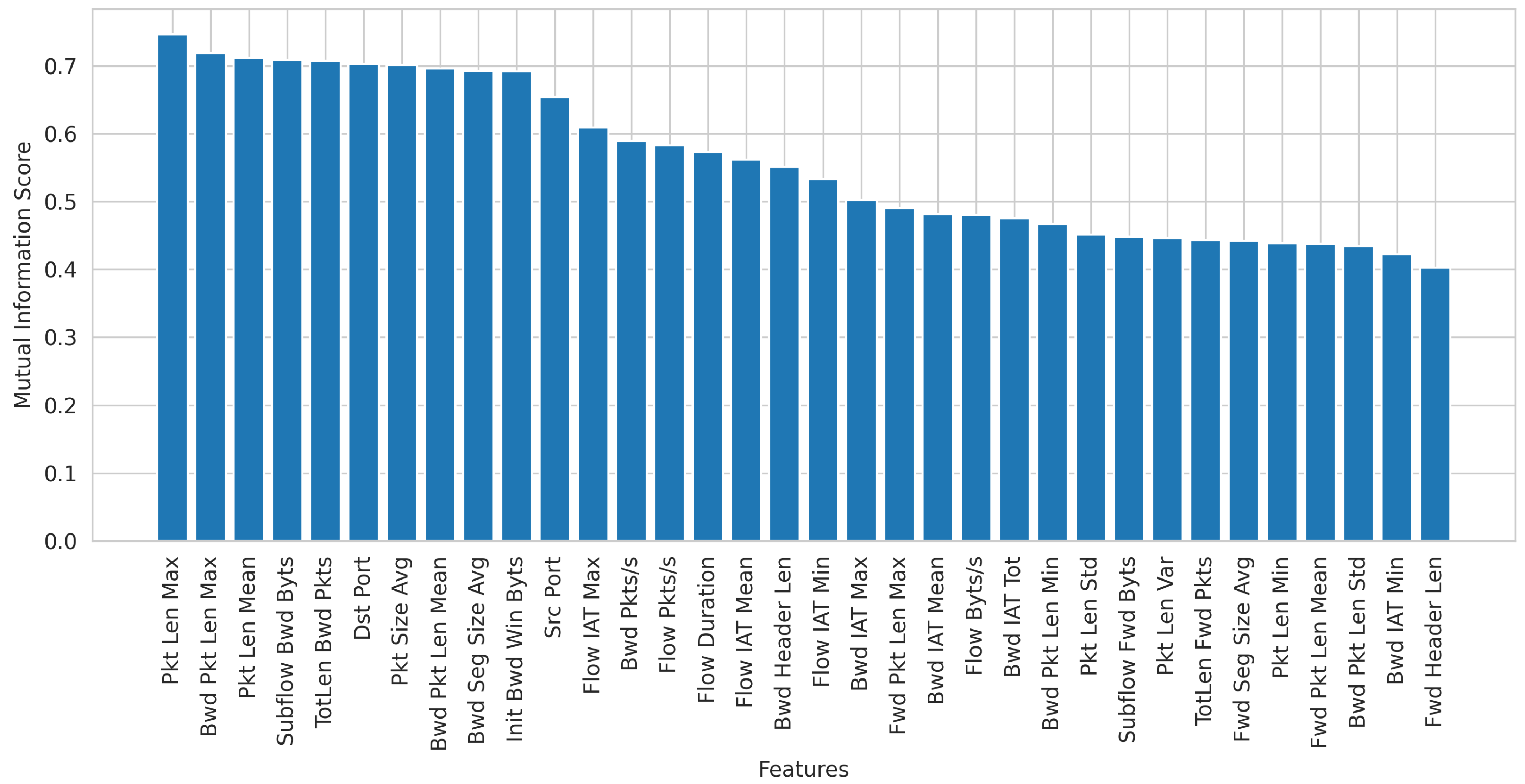
In the second stage, feature engineering was performed, which involved the application of the mutual information function. This function calculates the mutual information between each feature and the target variable in a classification problem. The function is based on the concepts of entropy and information theory. It means that a feature with a high mutual information score with the target variable provides valuable information for the classification task [36]. Two libraries, SelectKBest and mutual_info_classif from Scikit-learn [37], were utilized to conduct this analysis. A threshold of 0.40 was considered for feature selection, focusing on selecting the best features contributing to the model’s classification. The result of this process is depicted in Figure 2, with feature score values in descending order to visualize the most important features.

The previous sections aimed to evaluate the impact of each feature on the multiclass classification results. Therefore, analyzing the information obtained from SDN controllers using northbound interfaces is necessary, focusing explicitly on the study of APIs provided by the Ryu controller. This analysis is crucial in feature selection because classifiers can be implemented at the application layer of the SDN architecture. Although more features can be obtained from the controller, these should be evaluated and compared with the mutual information analysis performed before making the final decision. As a final result, five relevant features were obtained, which were used to train different DL models. The final selection of features is presented in

Table 5. Description of features.

No.	Feature Name	Description
1	Flow Duration	Duration of the flow in Microsecond
2	Flow Pkts/s	Number of flow bytes per second
3	Flow Byts/s	Number of flow packets per second
4	Fwd Pkts/s	Number of forward packets per second
5	Bwd Pkts/s	Number of backward packets per second

.

Table 6. Descriptive statistics.

	Flow Duration	Flow Pkts/s	Flow Byts/s	Fwd Pkts/s	Bwd Pkts/s
count	5.000000 $\times {10}^4$	5.000000 $\times {10}^4$	5.000000 $\times {10}^4$	5.000000 $\times {10}^4$	5.000000 $\times {10}^4$
mean	−2.387424 $\times {10}^{-17}$	1.136868 $\times {10}^{-18}$	−5.400557 $\times {10}^{-18}$	−7.389644 $\times {10}^{-18}$	−2.273737 $\times {10}^{-18}$
std	1.000010 $\times {10}^0$	1.000010 $\times {10}^0$	1.000010 $\times {10}^0$	1.000010 $\times {10}^0$	1.000010 $\times {10}^0$
min	−5.253012 $\times {10}^{-1}$	−1.000130 $\times {10}^{-1}$	−4.345196 $\times {10}^{-2}$	−5.722901 $\times {10}^{-2}$	−1.127359 $\times {10}^{-1}$
25%	−5.200939 $\times {10}^{-1}$	−9.993990 $\times {10}^{-2}$	−4.344642 $\times {10}^{-2}$	−5.722901 $\times {10}^{-2}$	−1.126813 $\times {10}^{-1}$
50%	−4.405559 $\times {10}^{-1}$	−9.982524 $\times {10}^{-2}$	−4.342988 $\times {10}^{-2}$	−5.714464 $\times {10}^{-2}$	−1.125122 $\times {10}^{-1}$
75%	−4.341171 $\times {10}^{-1}$	−9.591224 $\times {10}^{-2}$	−4.287239 $\times {10}^{-2}$	−5.707213 $\times {10}^{-2}$	−1.089045 $\times {10}^{-1}$
max	2.576183 $\times {10}^0$	4.561686 $\times {10}^1$	1.236910 $\times {10}^2$	3.544473 $\times {10}^1$	4.542805 $\times {10}^1$

shows the results of the descriptive statistics for the five selected features. This information provides a detailed view of the features of the standardized data. It is observed that measures of central tendency, such as the mean, are very close to zero for most of the features, suggesting a distribution centered around zero after standardization. Standard deviations close to one indicate similar dispersion across all features after standardization. Ranges and percentiles reveal variability in the data, with some features, such as “Flow Duration”, showing a much more comprehensive range than others. In addition, the presence of high values in “Flow Pkts/s” and “Bwd Pkts/s” is noted, with their maximum values significantly higher than the (75.00%) percentiles; however, these values are expected, as these are values in milliseconds. Overall, these results provide an in-depth understanding of the distribution and variability of the features.

3.4. Model

Various activities are carried out in this phase to construct and evaluate data models. Thus, it involves using and applying a series of modeling algorithms to classify the preprocessed data and assess their effectiveness in achieving the expected results. It focuses on constructing and training DL models using the data prepared in the modification phase.

3.4.1. Hardware and Software Environment

The experiment was executed using the Ubuntu 18.04 64-bit operating system, PyCharm Professional for remote connection to the RIG server, Python 3.10 programming language, and several libraries such as TensorFlow, Keras, NumPy, Pandas, and Scikit-Learn.

Table 7. Hardware description.

Component	Description
Processor	AMD Ryzen Threadrippe 2920X
Main board	ASUS ROG Zenith Extreme Alpha
RAM	64 GB Crucial Ballistix DDR4-3000
GPU	16 GB Phantom Gaming X Radeon VII
SSD	500 GB Crucial SSD M.2 NVMe
HDD	3 TB Western Digital HDD Purple

provides detailed hardware information about the RIG server.

3.4.2. Deep Learning Model Selection

The most commonly used DL algorithms for traffic classification in SDN are CNN, SAE, MLP, and LSTM [12,38]. The dataset used in this study exhibits temporal evolution in communication patterns over time. RNN algorithms perform better when dealing with time series problems and sequences, such as anomaly detection and network traffic classification. However, an RNN has different characteristics than other networks like CNN; its focus is on time series data. In other words, an RNN has directional connections that allow it to calculate the next step based on the previous steps [39]. Nevertheless, a simple RNN needs help to learn long-term relationships in data sequences. Therefore, for the development of the traffic classifier, four RNN-derived algorithms were employed: LSTM, BiLSTM, GRU, and BiGRU. These algorithms are designed to learn meaningful connections in longer sequences.

• GRU: These are variants of LSTM networks that incorporate a forgetting gate. Unlike LSTMs, GRUs have fewer parameters due to the absence of an output gate. Despite this difference, GRUs offer similar accuracy to LSTMs [40]. In addition, it has been observed that GRUs can offer computationally more efficient performance in certain scenarios. Figure 3 shows the architecture of the GRU model.

• BiGRU is a model that adds a future layer in the opposite direction of the data sequence. This network uses two hidden layers to extract past and future information connected to a single output layer. This bidirectional structure aids an RNN in removing more information, consequently enhancing the learning process’s performance [41]. Figure 4 shows the architecture of the BiGRU model.

• LSTM: It is a variant of RNNs that can perform computations based on time sequences, allowing the processing of recent data and data that occurred at distant time steps in the series. Unlike a simple RNN algorithm, LSTMs can assess the significance of data, even when there are many time steps between them, making them ideal for learning long-term relationships [42]. Figure 5 shows the architecture of the LSTM model.

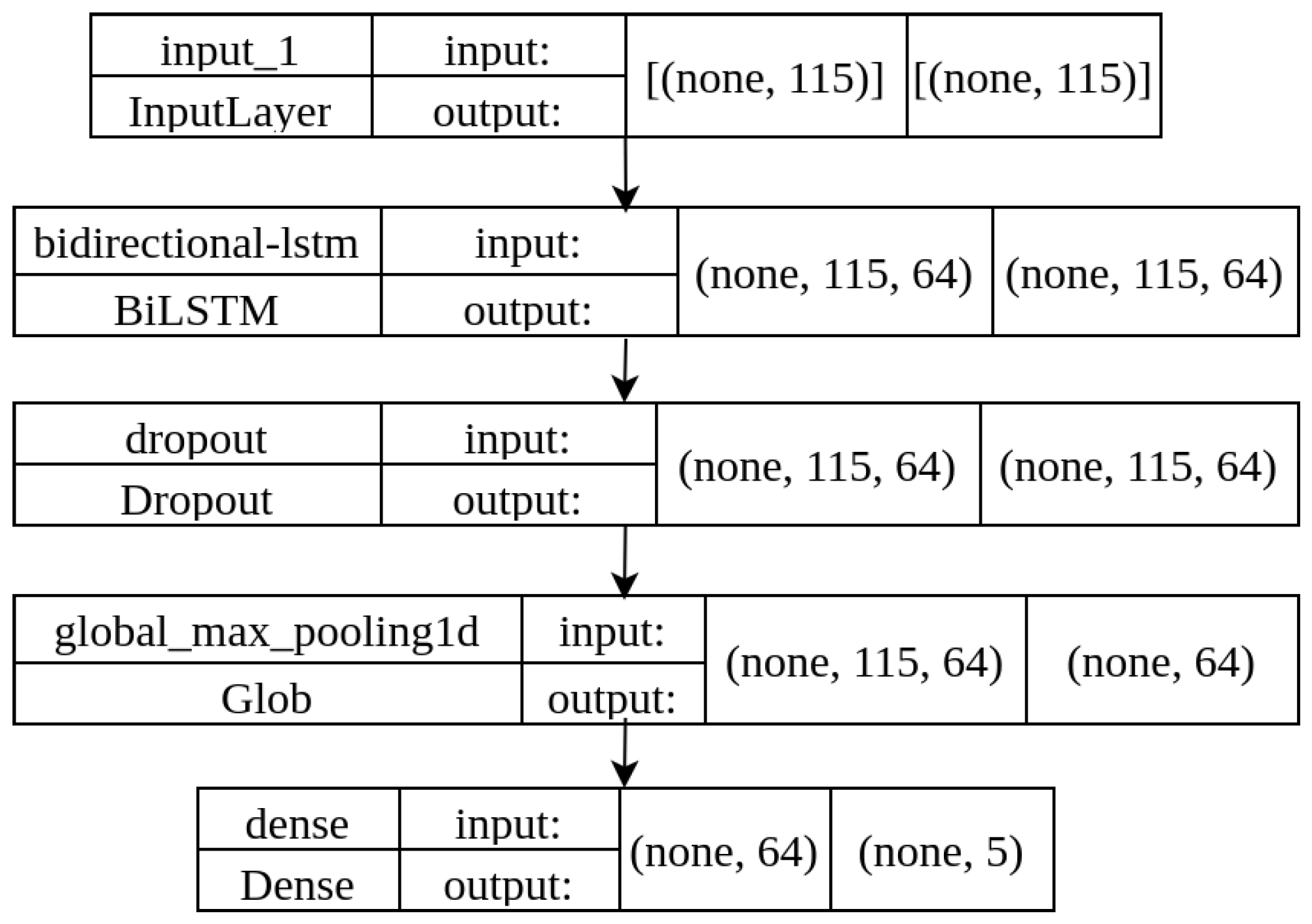
• BiLSTM: This model employs two LSTMs, one of which processes the sequence forward and the other in reverse. Through this bidirectional process, BiLSTM increases the amount of information available to the network, which can be valuable in traffic classification problems where comprehending relationships between various traffic features is essential [43]. Figure 6 shows the architecture of the BiLSTM model.

3.4.3. Definition of Hyperparameters

Once the DL models were defined, the dataset was split into 70.00% for training, 15.00% for validation, and 15.00% for testing. Next, optimal performance was evaluated through hyperparameter tuning. To define an RNN, a sequential network is created, which can be either unidirectional or bidirectional, followed by additional layers for multiclass classification. In particular, a layer with 64 neurons was added to the model, configured to return all sequences instead of a single value. A dropout layer with a dropout rate of 20.00% was included to prevent overfitting during training, as it randomly deactivates 20.00% of units at each step. A Global Max-Pooling 1D layer was introduced, extracting the maximum value along the temporal dimension to reduce the output dimensionality of the RNN layer. Then, a dense layer with five neurons, each corresponding to one of the predefined classes in the sample section, and a softmax activation function were added. The softmax activation layer transforms the outputs into probability distributions for each class. During the training stage for all models, the categorical_crossentropy loss function was employed, with 20 training epochs and the ’adam’ optimizer, and model performance was evaluated using the accuracy metric, given that it is a multiclass classification problem. All parameters used during the experimentation are detailed in

Table 8. Hyperparameter setup.

Activation Function	Loss Function	Bath Size	Optimization Algorithm	Input Layer	No. Epochs
Sigmoid	Categorical crossentropy	16	Adam	64	20

.

3.5. Assess

It is the final phase of the SEMMA methodology. One of the most critical steps in machine learning models is their evaluation, which means determining their performance. Metrics provide information about the performance and accuracy of each model [44]. In this section, the performance of the four models is evaluated using test data, which means data that were not used during the training phase. Multiple metrics were employed to measure their performance and assess their predictive capability. Different evaluation metrics exist depending on the type of technique applied. In this case, the classification metrics used were Accuracy (2), Precision (3), Recall (4), and F1-Score (5), which were used to gain a broader understanding of each model’s behavior and how well it fits the data.

• Accuracy is the model’s precision in predicting accurate outcomes, calculated by dividing the number of accurate predictions by the total number of predictions.

  $$\begin{array}{cc}\hfill Accuracy& =\frac{TP+TN}{TP+TN+FP+FN}\hfill \end{array}$$

  (2)
• Precision indicates how precise the model is in identifying positive cases. It is calculated by dividing the number of correctly classified positive instances by the total number of cases classified as positive.

  $$\begin{array}{cc}\hfill Precision& =\frac{TP}{TP+FP}\hfill \end{array}$$

  (3)
• Recall is the proportion of positive cases correctly identified by dividing the number of correctly classified positive instances by the total number of positive cases.

  $$\begin{array}{cc}\hfill Recall& =\frac{TP}{TP+FN}\hfill \end{array}$$

  (4)
• F1-Score aims to achieve a balanced performance in classifying positive and negative cases. It is a combined measure of precision and recall that balances both metrics. This metric was helpful because there was an imbalance in the classes.

  $$\begin{array}{cc}\hfill F1\text{-}Score& =2\ast \frac{Precision\ast Recall}{Precision+Recall}\hfill \end{array}$$

  (5)

4. Results and Discussion

This section presents and interprets the results of deploying the four DL algorithms. However, it is crucial to determine the sequence length to be fed into the algorithms before applying them.

4.1. Sequence Length Analysis Results

The analysis of sequence length was conducted by running several tests. Based on these tests, three sequence length values were defined: sequence_length = 50, sequence_length = 75, and sequence_length = 115. Once these values were determined, the four DL models were executed. The results of these tests are presented in

Table 9. Sequence length analysis.

Algorithm	Sequence Length	Training Accuracy	Test Accuracy	Training Time (s)
GRU	50	0.9711	0.9744	244
BiGRU	50	0.9824	0.9492	382
LSTM	50	0.9639	0.9582	229
BiLSTM	50	0.9607	0.6023	424
GRU	75	0.9894	0.9834	251
BiGRU	75	0.9900	0.9553	390
LSTM	75	0.9825	0.9782	317
BiLSTM	75	0.9859	0.8644	540
GRU	115	0.9927	0.9955	339
BiGRU	115	0.9904	0.9854	626
LSTM	115	0.9853	0.9951	382
BiLSTM	115	0.9843	0.8777	646

.

Table 9 presents each DL algorithm’s training accuracy, test accuracy, and training times with different sequence lengths. During the training phase, it was observed that GRU and BiGRU consistently yielded the highest evaluation accuracy. However, in the evaluation phase, the best results were obtained with GRU and LSTM, while the lowest performance was consistently observed with BiLSTM. Regarding the training times for each DL algorithm in our model, it was noted that GRU was trained in 297 s and LSTM in 289 s. Consequently, it was determined that the optimal sequence length is 115.

4.2. Evaluation of the Classifiers

In this section, we present the results of traffic classification by the four selected DL models, utilizing the established hyperparameters from the modeling phase and sequence lengths defined in the previous section. The evaluation metrics include accuracy, precision, recall, and F1 score. We present detailed results with all evaluation metrics in

Table 10. Evaluation metrics of the proposed models.

Algorithm	Accuracy	Precision	Recall	F1-Score	Training Time (s)	GPU Utilization (%)
GRU	0.9965	Class 0: 1.00 Class 1: 1.00 Class 2: 1.00 Class 3: 1.00 Class 4: 1.00	Class 0: 0.94 Class 1: 0.99 Class 2: 0.93 Class 3: 0.99 Class 4: 0.98	Class 0: 0.97 Class 1: 0.99 Class 2: 0.96 Class 3: 1.00 Class 4: 0.99	339	28
BiGRU	0.9860	Class 0: 1.00 Class 1: 1.00 Class 2: 1.00 Class 3: 1.00 Class 4: 1.00	Class 0: 0.94 Class 1: 0.98 Class 2: 0.85 Class 3: 0.95 Class 4: 0.86	Class 0: 0.97 Class 1: 0.99 Class 2: 0.92 Class 3: 0.97 Class 4: 0.92	626	45
LSTM	0.9963	Class 0: 1.00 Class 1: 1.00 Class 2: 1.00 Class 3: 1.00 Class 4: 1.00	Class 0: 0.94 Class 1: 0.99 Class 2: 0.88 Class 3: 0.99 Class 4: 0.98	Class 0: 0.97 Class 1: 0.99 Class 2: 0.94 Class 3: 1.00 Class 4: 0.99	389	33
BiLSTM	0.9932	Class 0: 0.99 Class 1: 0.93 Class 2: 0.97 Class 3: 0.99 Class 4: 0.91	Class 0: 0.73 Class 1: 0.70 Class 2: 0.64 Class 3: 0.70 Class 4: 0.80	Class 0: 0.84 Class 1: 0.80 Class 2: 0.77 Class 3: 0.82 Class 4: 0.85	646	48

.

4.3. Discussion

After running each algorithm, this subsection presents the graphical analysis with the defined hyperparameters and a sequence length of 115. The GRU, BiGRU, and LSTM algorithms generalized correctly, as the training precision values obtained in each model were close to their respective validation precision values.

4.3.1. GRU Model

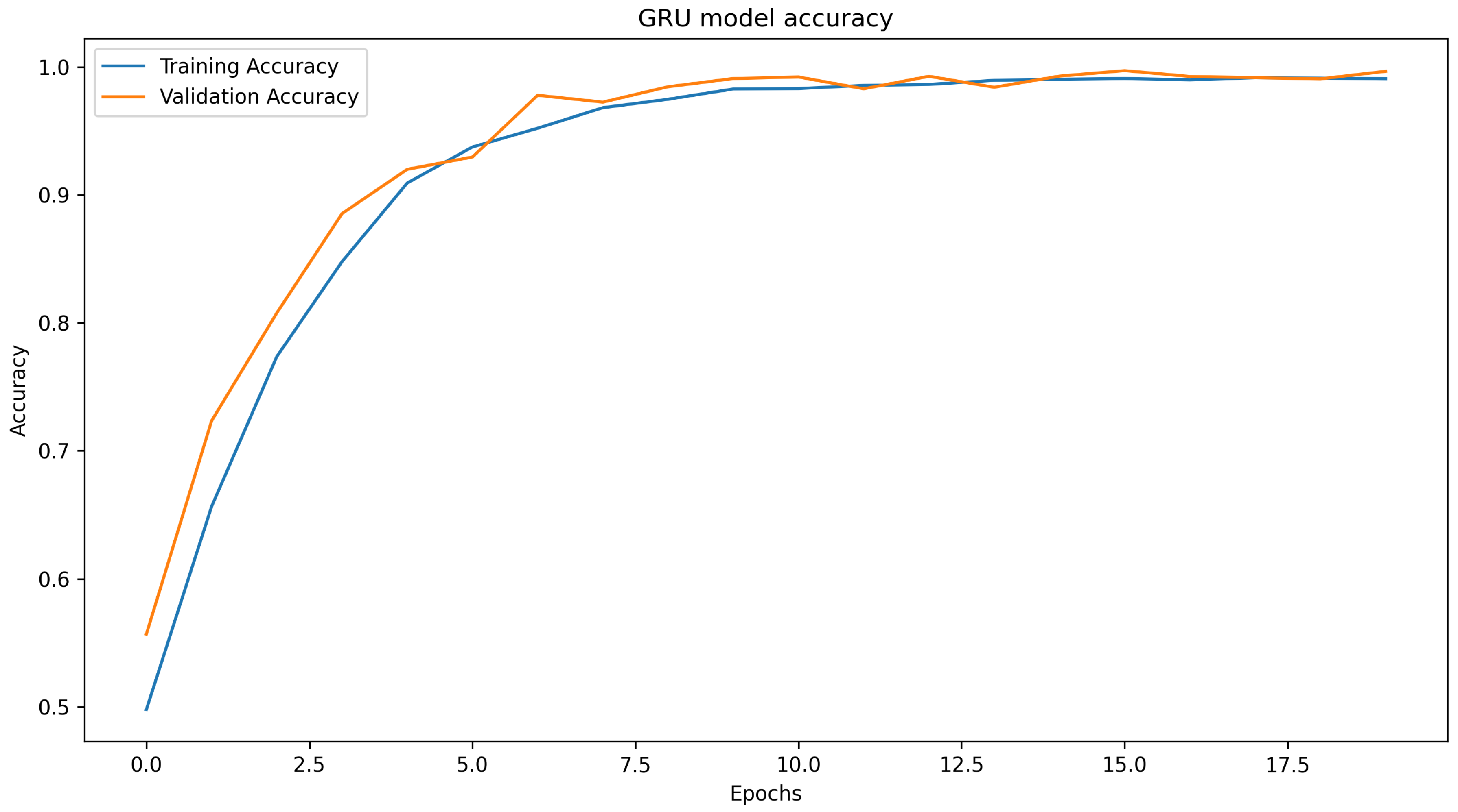
Figure 7 shows that the accuracy achieved with GRU at 20 epochs in the training set is (99.07%), while, in the validation set, it is (99.65%). Although there is a slight difference between the accuracy of the training set and the validation set (0.58%), this gap is minimal, indicating effective generalization of the model. The overall trend shows a steady increase in accuracy and a decrease in loss across epochs, supporting the effectiveness of the training and the ability of the model to learn and generalize to unseen data.

The F1-score, which combines precision and recall, performed highly in all classes, with values ranging from (96.00%) to (100%). Specifically, classes 1 and 3 had a perfect F1-score of 1.00, while classes 0 and 2 had very high F1-scores of (97.00%) and (96.00%), respectively. The precision per class was (100%), indicating no false positives for any class. On the other hand, recall varied slightly between classes, with values ranging from (93.00%) to (99.00%). This suggests that, although the model correctly classified the vast majority of instances of all classes, some instances of classes 0 and 2 needed to be correctly classified, as indicated by the slightly lower recall for those classes. These results indicate exceptionally high model performance on the multiclass classification task.

The training time of the model was 339 s. During the training process, (28.00%) of the GPU was used, suggesting an efficient utilization of the available hardware resources to speed up the training process. This moderate GPU usage also indicates that the model did not require an intensive workload regarding computational resources, which benefits the scalability and efficiency of training in resource-constrained production environments.

4.3.2. BiGRU Model

Figure 8 shows that the accuracy achieved with BiGRU at 20 epochs in the training dataset is (99.34%); the model undergoes significant growth until reaching a final accuracy of (98.60%) with the validation dataset. This increase in accuracy is accompanied by a steady decrease in loss, indicating a continuous improvement in the model’s predictive ability. Although some fluctuations in performance are observed during training, the model manages to stabilize towards the end of the process, demonstrating effective learning and an ability to generalize well to unseen data.

The F1-score generally performed well in most classes, ranging from (92.00%) to (99.00%). Specifically, classes 1 and 3 achieved F1 scores of (99.00%) and (97.00%), respectively, indicating high precision and recall in classifying those classes. Class precision was (100%), suggesting no false positives for any class. However, recall varied between classes, with values ranging from (85.00%) to (98.00%), indicating that the model had difficulty recovering all instances of classes 2 and 4 compared to the other classes. Overall, the model showed good performance in most classes, although there could be room for improvement in the recovery of some specific classes.

The total model training time was 626 s. During this process, (45.00%) of the GPU was utilized, indicating a moderate but significant use of available hardware resources to accelerate model training. This percentage of GPU utilization suggests efficient resource allocation.

4.3.3. LSTM Model

Figure 9 shows that the accuracy achieved with LSTM at 20 epochs in the training set is (98.86%), while in the validation set it is (99.63%). Although there is a difference between the accuracy of the training set and the validation set (0.77%), this gap is minimal, indicating effective generalization of the model. The overall trend shows a steady increase in accuracy and a decrease in loss across epochs, supporting the effectiveness of the training and the ability of the model to learn and generalize to unseen data. On the other hand, loss shows a steady downward trend, indicating a continuous improvement in the model’s ability to fit the data. These results suggest successful training, with the model achieving high accuracy and low loss on both datasets.

The F1-score showed high performance in all classes, with values ranging from (94.00%) to (100%). Specifically, classes 1, 3, and 4 achieved an F1-score of (99.00%) and (100%), respectively, indicating high precision and recall in classifying those classes. The precision per class was (100%), suggesting no false positives for any class. However, recall varied between classes, with values ranging from (88.00%) to (99.00%), indicating that the model had some difficulty recovering all instances of class 2 compared to the other classes. Overall, the model performed well in most classes, with high accuracies, F1-score, and recall, suggesting a robust ability to classify the different classes correctly.

The total training time of the model was 389 s. During this process, (33.00%) of the graphics processing unit (GPU) was utilized, indicating a moderate use of available hardware resources to accelerate model training. This percentage of GPU utilization suggests efficient resource allocation and an appropriate workload for the training task.

4.3.4. BiLSTM Model

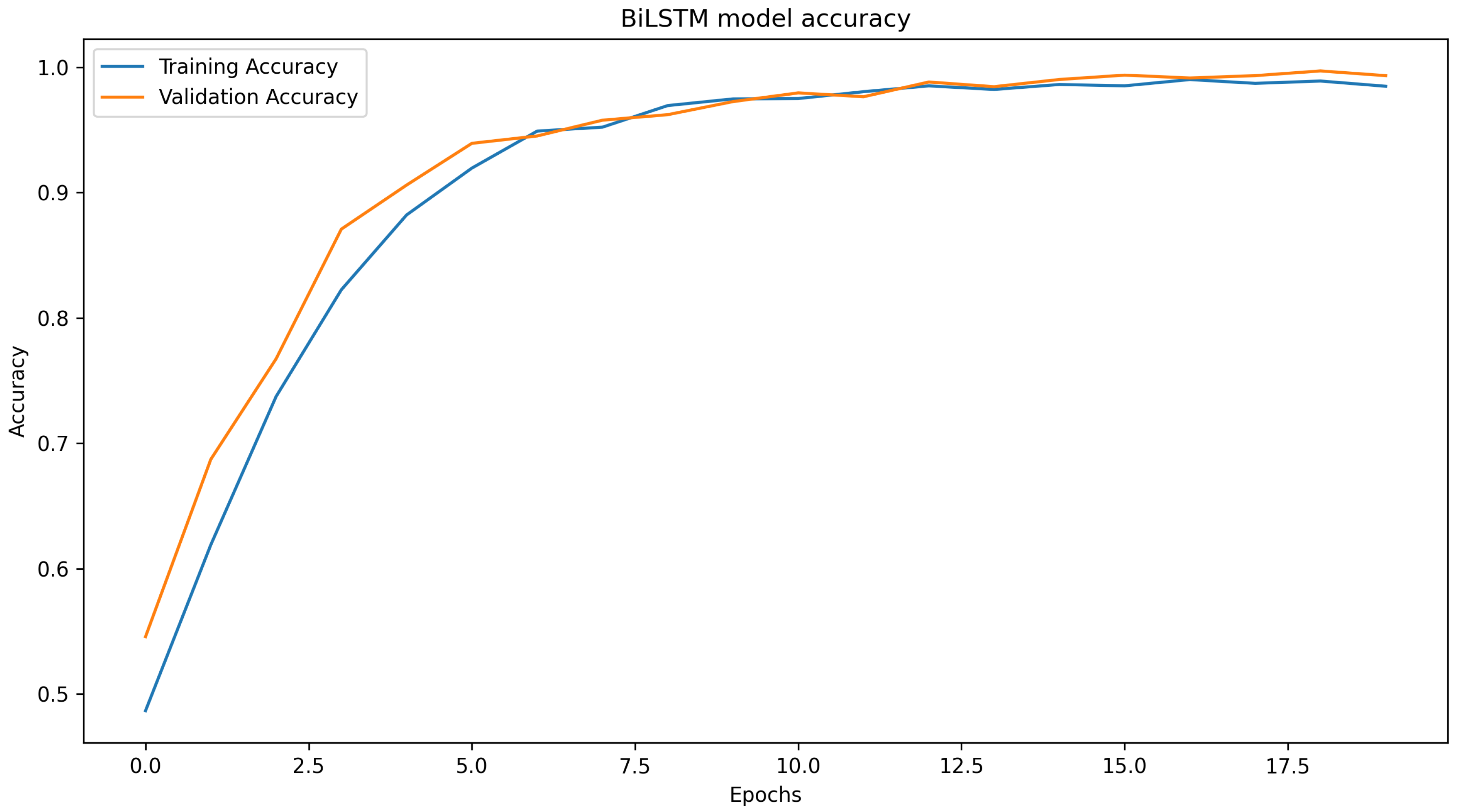
Figure 10 shows that the accuracy achieved with BiLSTM at 20 epochs in the training set is (98.47%), while in the validation set, it is (99.32%). This increase in accuracy is accompanied by a steady decrease in loss, indicating a continuous improvement in the model’s ability to fit the data. These results suggest successful training, with the model achieving high accuracy and low loss on both datasets.

The F1-score showed varying performance across the different classes, with values ranging from (77.00%) to (85.00%). Classes 0 and 4 showed the highest F1-score, with (84.00%) and (85.00%), respectively, while classes 1 and 2 had the lowest F1-score, with (80.00%) and (77.00%), respectively. The precision by class also varied, ranging from (91.00%) to (99.00%). Class 0 had the highest precision (99.00%), followed by classes 3 and 2. Class 1 had the lowest precision (93.00%). As for the recall per class, the values varied between (64.00%) and (80.00%). Class 4 had the highest recall (80.00%), while class 2 had the lowest recall (64.00%). These metrics show that the model has generally acceptable performance, although there may be room for improvement in some specific classes, especially in classes 1 and 2, where the F1-score was lower.

The total model training time was 646 s. During this process, (48.00%) of the GPU was utilized, indicating a considerable use of available hardware resources to accelerate model training; this may result in a faster and more efficient training process than using only the CPU.

4.4. Comparative Assessment of Model Performance

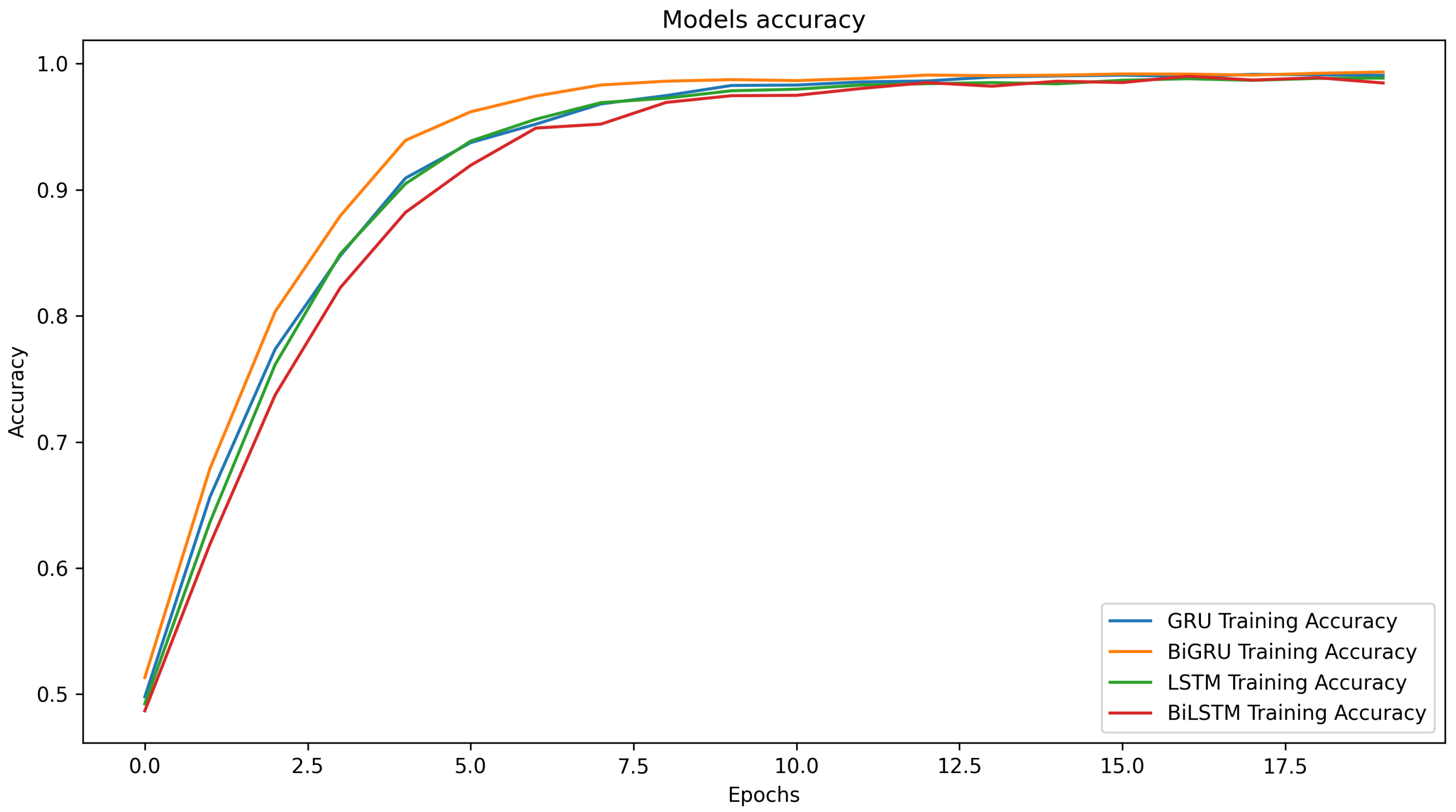
Figure 11 shows the four models, GRU, BiGRU, LSTM, and BiLSTM, which were trained and evaluated with training and validation datasets. Based on the information provided, the model that generalizes best is the GRU model. This model achieves very high accuracy on the training set (99.07%) and the validation set (99.65%), with minimal difference between the two sets. This minimal difference suggests that the GRU model can generalize effectively to unseen data, indicating a robust ability to learn general patterns in the data. Although the LSTM, BiGRU, and BiLSTM models also show high accuracy and minimal difference between the training and validation sets, the GRU model slightly outperforms them regarding accuracy on the validation set. Therefore, regarding generalization, the GRU model is the most effective of the four models evaluated.

The F1-score analysis shows different performance levels; the GRU model showed high performance in all classes, with the F1-score ranging from (96.00%) to (100%), and perfect precision in all classes. Although the BiGRU model also showed generally high performance, with the F1-score ranging from (92.00%) to (99.00%), some difficulties in instance recall were observed in certain classes, particularly in classes 2 and 4. On the other hand, both the LSTM and BiLSTM models exhibited variability in performance across classes, with some challenges in precision and recall in certain classes. All GRU and LSTM models showed solid and consistent performance across all classes. In contrast, the BiGRU and BiLSTM models showed some variability and possible areas for improvement, such as recall in some specific classes.

In the analysis of training time and GPU usage, we observed that all models efficiently used the available hardware resources to accelerate the training process. The GRU and LSTM models showed moderate GPU usage, with utilization percentages of (28.00%) and (33.00%), respectively, indicating adequate resource allocation and appropriate workload for the training task. However, the BiGRU and BiLSTM models demonstrated more significant GPU utilization, with (45.00%) and (48.00%), respectively. While this might suggest a more intensive utilization of hardware resources, it also indicates an efficient allocation of resources to accelerate model training. Overall, all models obtained reasonable training times and efficient GPU utilization; this demonstrates their ability to handle an efficient workload and perform practical training in resource-constrained environments.

4.5. Comparison with Previous Research

Table 11. Accuracy comparison with previous research on traffic classification.

Ref.	Algorithm	Accuracy	Number of Features
Proposed	GRU BiGRU LSTM BiLSTM	99.65% 98.60% 99.63% 99.32%	5
[18]	ML-LSTM SAE CNN	97.14% 99.14% 99.30%	Automatic by algorithm
[19]	SAE	>90.00%	Automatic by algorithm
[20]	ML-LSTM	97.14%	Automatic by algorithm
[21]	CNN MLP SAE	93.35% 93.21% 93.13%	4
[22]	CNN DNN	96.00% 94.00%	23
[23]	CNN+autoencoder CNN DNN	97.42% 96.03% 94.36%	Flow features selected by autoencoders
[24]	GAN CNN	93.18% 93.30%	Automatic by algorithm
[25]	CNN LSTM SAE	98.85% 99.22% 98.74%	Automatic by algorithm
[26]	MLP, CNN and SAE	>90.00%	Automatic by algorithm
[27]	ResNet	97.24%	20
[28]	VAE	89.00%	6

compares the accuracy of the proposed models and other approaches developed by researchers. As can be seen, our GRU and LSTM models achieve higher accuracy with fewer features than all methods using deep learning. Furthermore, our LSTM model achieves higher accuracy than LSTM models [18,25], which use features selected automatically by the algorithm. However, it is essential to note that the GRU model achieves superior accuracy to LSTM. This accuracy highlights the efficiency and performance of our model compared to other existing approaches, outperforming previously developed LSTM models. Thus, the implementation of the GRU architecture can result in further improvements in SDN traffic classification accuracy.

5. Conclusions

This research develops a model for traffic classification by application types and network attacks using DL techniques to enhance QoS and security in SDN. The classifiers identify application types and attacks in five classes: Multimedia, VoIP, Instant message, File transfer, and Attacks. The SEMMA methodology was conducted to develop accurate models and obtain reliable results. We trained the models with four derived RNN algorithms, GRU, BiGRU, LSTM, and BiLSTM, which were evaluated during this process. Each model performed traffic classification using two open datasets, VPN–nonVPN and InSDN, extracting flows with a 15 s timeout with the CICFlowMeter tool. It resulted in a dataset of 50,000 samples, with 10,000 samples per class representing different types of applications and attacks. We selected five features to train the models based on analyzing the features obtainable from the SDN controller’s northbound interface and conducting mutual information analysis. We determined the length of the sequence through several experiments. The accuracy results for each model were as follows: GRU (99.65%), BiGRU (98.60%), LSTM (99.63%), and BiLSTM (99.32%). These results underscore the remarkable effectiveness of the GRU model in traffic classification. These findings provide great potential for improving the security and QoS in SDN employing traffic classification, contributing to network administration.

Although deep learning has been used to develop the classifiers, developing new applications or attacks could affect their effectiveness. In addition, the datasets used may only partially reflect the complexity of traffic in real environments. Therefore, as future work, we will seek to implement the proposed classifiers in a real-time SDN environment to instantaneously classify incoming flows based on the statistical information of the flows and apply corresponding QoS, and security policies.

References

1. Cisco. Cisco Annual Internet Report (2018–2023); Technical Report; Cisco: San Jose, CA, USA, 2018–2023; Available online: www.cisco.com/c/en/us/solutions/collateral/executive-perspectives/annual-internet-report/white-paper-c11-741490.html (accessed on 1 April 2024).
2. Belkadi, O.; Vulpe, A.; Laaziz, Y.; Halunga, S. ML-Based Traffic Classification in an SDN-Enabled Cloud Environment. Electronics 2023, 12, 269. [Google Scholar] [CrossRef]
3. Ayoubi, S.; Limam, N.; Salahuddin, M.A.; Shahriar, N.; Boutaba, R.; Estrada-Solano, F.; Caicedo, O.M. Machine Learning for Cognitive Network Management. IEEE Commun. Mag. 2018, 56, 158–165. [Google Scholar] [CrossRef]
4. Clark, D.D.; Partridge, C.; Ramming, J.C.; Wroclawski, J.T. A Knowledge Plane for the Internet. In Proceedings of the 2003 Conference on Applications, Technologies, Architectures, and Protocols for Computer Communications, SIGCOMM’03, New York, NY, USA, 25–29 August 2003; pp. 3–10. [Google Scholar] [CrossRef]
5. Trois, C.; Del Fabro, M.D.; de Bona, L.C.E.; Martinello, M. A Survey on SDN Programming Languages: Toward a Taxonomy. IEEE Commun. Surv. Tutor. 2016, 18, 2687–2712. [Google Scholar] [CrossRef]
6. Kreutz, D.; Ramos, F.M.V.; Veríssimo, P.E.; Rothenberg, C.E.; Azodolmolky, S.; Uhlig, S. Software-Defined Networking: A Comprehensive Survey. Proc. IEEE 2015, 103, 14–76. [Google Scholar] [CrossRef]
7. Xie, J.; Yu, F.R.; Huang, T.; Xie, R.; Liu, J.; Wang, C.; Liu, Y. A Survey of Machine Learning Techniques Applied to Software Defined Networking (SDN): Research Issues and Challenges. IEEE Commun. Surv. Tutor. 2019, 21, 393–430. [Google Scholar] [CrossRef]
8. Moore, A.W.; Papagiannaki, K. Toward the Accurate Identification of Network Applications. In Passive and Active Network Measurement; Dovrolis, C., Ed.; Springer: Berlin/Heidelberg, Germany, 2005; pp. 41–54. [Google Scholar]
9. Nguyen, T.T.; Armitage, G. A survey of techniques for internet traffic classification using machine learning. IEEE Commun. Surv. Tutor. 2008, 10, 56–76. [Google Scholar] [CrossRef]
10. Finsterbusch, M.; Richter, C.; Rocha, E.; Muller, J.A.; Hanssgen, K. A Survey of Payload-Based Traffic Classification Approaches. IEEE Commun. Surv. Tutor. 2014, 16, 1135–1156. [Google Scholar] [CrossRef]
11. Li, G.; Dong, M.; Ota, K.; Wu, J.; Li, J.; Ye, T. Deep Packet Inspection Based Application-Aware Traffic Control for Software Defined Networks. In Proceedings of the 2016 IEEE Global Communications Conference (GLOBECOM), Washington, DC, USA, 4–8 December 2016; pp. 1–6. [Google Scholar] [CrossRef]
12. Nunez-Agurto, D.; Fuertes, W.; Marrone, L.; Macas, M. Machine Learning-Based Traffic Classification in Software-Defined Networking: A Systematic Literature Review, Challenges, and Future Research Directions. IAENG Int. J. Comput. Sci. 2022, 49, 1002–1015. [Google Scholar]
13. Fan, Z.; Liu, R. Investigation of machine learning based network traffic classification. In Proceedings of the 2017 International Symposium on Wireless Communication Systems (ISWCS), Bologna, Italy, 28–31 August 2017; pp. 1–6. [Google Scholar]
14. Tahaei, H.; Afifi, F.; Asemi, A.; Zaki, F.; Anuar, N.B. The rise of traffic classification in IoT networks: A survey. J. Netw. Comput. Appl. 2020, 154, 102538. [Google Scholar] [CrossRef]
15. Hayes, M.; Ng, B.; Pekar, A.; Seah, W.K.G. Scalable Architecture for SDN Traffic Classification. IEEE Syst. J. 2018, 12, 3203–3214. [Google Scholar] [CrossRef]
16. Selvi, D.K.T.; Thamilselvan, R. Deep Learning Based Traffic Classification In Software Defined Networking—A Survey. Int. J. Sci. Technol. Res. 2020, 9, 2034–2041. [Google Scholar]
17. Md. Zaki, F.A.; Chin, T.S. FWFS: Selecting Robust Features Towards Reliable and Stable Traffic Classifier in SDN. IEEE Access 2019, 7, 166011–166020. [Google Scholar] [CrossRef]
18. Wang, P.; Ye, F.; Chen, X.; Qian, Y. Datanet: Deep Learning Based Encrypted Network Traffic Classification in SDN Home Gateway. IEEE Access 2018, 6, 55380–55391. [Google Scholar] [CrossRef]
19. Zhang, C.; Wang, X.; Li, F.; He, Q.; Huang, M. Deep learning–based network application classification for SDN. Trans. Emerg. Telecommun. Technol. 2018, 29, e3302. [Google Scholar] [CrossRef]
20. Lim, H.K.; Kim, J.B.; Kim, K.; Hong, Y.G.; Han, Y.H. Payload-Based Traffic Classification Using Multi-Layer LSTM in Software Defined Networks. Appl. Sci. 2019, 9, 2550. [Google Scholar] [CrossRef]
21. Chang, L.H.; Lee, T.H.; Chu, H.C.; Su, C.W. Application-Based Online Traffic Classification with Deep Learning Models on SDN Networks. Adv. Technol. Innov. 2020, 5, 216–229. [Google Scholar] [CrossRef]
22. Abdulazzaq, S.; Demirci, M. A Deep Learning Based System for Traffic Engineering in Software Defined Networks. Int. J. Intell. Syst. Appl. Eng. 2020, 8, 206–213. [Google Scholar] [CrossRef]
23. Chiu, K.C.; Liu, C.C.; Chou, L.D. CAPC: Packet-Based Network Service Classifier With Convolutional Autoencoder. IEEE Access 2020, 8, 218081–218094. [Google Scholar] [CrossRef]
24. Wang, P.; Wang, Z.; Ye, F.; Chen, X. ByteSGAN: A semi-supervised Generative Adversarial Network for encrypted traffic classification in SDN Edge Gateway. Comput. Netw. 2021, 200, 108535. [Google Scholar] [CrossRef]
25. Wu, H.; Zhang, X.; Yang, J. Deep Learning-Based Encrypted Network Traffic Classification and Resource Allocation in SDN. J. Web Eng. 2021, 20, 2319–2334. [Google Scholar] [CrossRef]
26. Setiawan, R.; Ganga, R.R.; Velayutham, P.; Thangavel, K.; Sharma, D.K.; Rajan, R.; Krishnamoorthy, S.; Sengan, S. Encrypted Network Traffic Classification and Resource Allocation with Deep Learning in Software Defined Network. Wirel. Pers. Commun. 2022, 127, 749–765. [Google Scholar] [CrossRef]
27. Ahn, S.; Kim, J.; Park, S.Y.; Cho, S. Explaining Deep Learning-Based Traffic Classification Using a Genetic Algorithm. IEEE Access 2021, 9, 4738–4751. [Google Scholar] [CrossRef]
28. Jang, Y.; Kim, N.; Lee, B.D. Traffic classification using distributions of latent space in software-defined networks: An experimental evaluation. Eng. Appl. Artif. Intell. 2023, 119, 105736. [Google Scholar] [CrossRef]
29. Azevedo, A.; Santos, M. KDD, semma and CRISP-DM: A parallel overview. In Proceedings of the IADIS European Conference on Data Mining, Amsterdam, The Netherlands, 24–26 July 2008; pp. 182–185. [Google Scholar]
30. Elsayed, M.S.; Le-Khac, N.A.; Jurcut, A.D. InSDN: A Novel SDN Intrusion Dataset. IEEE Access 2020, 8, 165263–165284. [Google Scholar] [CrossRef]
31. Draper-Gil, G.; Lashkari, A.H.; Mamun, M.S.I.; Ghorbani, A. Characterization of Encrypted and VPN Traffic using Time-related Features. In Proceedings of the 2nd International Conference on Information Systems Security and Privacy—ICISSP, Rome, Italy, 19–21 February 2016; pp. 407–414. [Google Scholar] [CrossRef]
32. Lashkari, A.H.; Gil, G.D.; Mamun, M.S.I.; Ghorbani, A.A. Characterization of Tor Traffic using Time based Features. In Proceedings of the 3rd International Conference on Information Systems Security and Privacy—ICISSP, Porto, Portugal, 19–21 February 2017; Volume 1, pp. 253–262. [Google Scholar] [CrossRef]
33. Chuang, H.M.; Liu, F.; Tsai, C.H. Early Detection of Abnormal Attacks in Software-Defined Networking Using Machine Learning Approaches. Symmetry 2022, 14, 1178. [Google Scholar] [CrossRef]
34. Garcia, C.; Leite, D.; Škrjanc, I. Incremental Missing-Data Imputation for Evolving Fuzzy Granular Prediction. IEEE Trans. Fuzzy Syst. 2020, 28, 2348–2362. [Google Scholar] [CrossRef]
35. Wang, H.; Bah, M.J.; Hammad, M. Progress in Outlier Detection Techniques: A Survey. IEEE Access 2019, 7, 107964–108000. [Google Scholar] [CrossRef]
36. Najafabadi, M.M.; Villanustre, F.; Khoshgoftaar, T.M.; Seliya, N.; Wald, R.; Muharemagic, E. Deep learning applications and challenges in big data analytics. J. Big Data 2015, 2, 1. [Google Scholar] [CrossRef]
37. George, B. A study of the effect of random projection and other dimensionality reduction techniques on different classification methods. Baselius Res. 2017, 18, 201769. [Google Scholar]
38. Nuñez-Agurto, D.; Fuertes, W.; Marrone, L.; Benavides-Astudillo, E.; Vásquez Bermúdez, M. Traffic Classification in Software-Defined Networking by Employing Deep Learning Techniques: A Systematic Literature Review. In Technologies and Innovation, 9th International Conference, CITI 2023, Guayaquil, Ecuador, 13–16 November 2023; Springer: Cham, Switzerland, 2023; pp. 67–80. [Google Scholar]
39. Deng, H.; Zhang, L.; Shu, X. Feature memory-based deep recurrent neural network for language modeling. Appl. Soft Comput. 2018, 68, 432–446. [Google Scholar] [CrossRef]
40. Cao, X.; Zhong, Y.; Zhou, Y.; Wang, J.; Zhu, C.; Zhang, W. Interactive Temporal Recurrent Convolution Network for Traffic Prediction in Data Centers. IEEE Access 2018, 6, 5276–5289. [Google Scholar] [CrossRef]
41. Li, H.; He, E.; Kuang, C.; Yang, X.; Wu, X.; Jia, Z. An Abnormal Traffic Detection Based on Attention-Guided Bidirectional GRU. In Proceedings of the 2022 IEEE 22nd International Conference on Communication Technology (ICCT), Nanjing, China, 11–14 November 2022; pp. 1300–1305. [Google Scholar] [CrossRef]
42. Hochreiter, S.; Schmidhuber, J. Long Short-Term Memory. Neural Comput. 1997, 9, 1735–1780. [Google Scholar] [CrossRef] [PubMed]
43. Xu, H.; Sun, L.; Fan, G.; Li, W.; Kuang, G. A Hierarchical Intrusion Detection Model Combining Multiple Deep Learning Models With Attention Mechanism. IEEE Access 2023, 11, 66212–66226. [Google Scholar] [CrossRef]
44. Vinayakumar, R.; Alazab, M.; Srinivasan, S.; Pham, Q.V.; Padannayil, S.K.; Simran, K. A Visualized Botnet Detection System Based Deep Learning for the Internet of Things Networks of Smart Cities. IEEE Trans. Ind. Appl. 2020, 56, 4436–4456. [Google Scholar] [CrossRef]
Figure 1. SEMMA process.
Futureinternet 16 00153 g001
Figure 2. Mutual information score.
Futureinternet 16 00153 g002
Figure 3. GRU model architecture.
Futureinternet 16 00153 g003
Figure 4. BiGRU model architecture.
Futureinternet 16 00153 g004
Figure 5. LSTM model architecture.
Futureinternet 16 00153 g005
Figure 6. BiLSTM model architecture.
Futureinternet 16 00153 g006
Figure 7. GRU accuracy.
Futureinternet 16 00153 g007
Figure 8. BiGRU accuracy.
Futureinternet 16 00153 g008
Figure 9. LSTM accuracy.
Futureinternet 16 00153 g009
Figure 10. BiLSTM accuracy.
Futureinternet 16 00153 g010
Figure 11. Models’ Accuracy.
Futureinternet 16 00153 g011