Efficient Integration of Heterogeneous Mobility-Pollution Big Data for Joint Analytics at Scale with QoS Guarantees

Abstract

Numerous real-life smart city application scenarios require joint analytics on unified views of georeferenced mobility data with environment contextual data including pollution and meteorological data. particularly, future urban planning requires restricting vehicle access to specific areas of a city to reduce the adverse effect of their engine combustion emissions on the health of dwellers and cyclers. Current editions of big spatial data management systems do not come with over-the-counter support for similar scenarios. To close this gap, in this paper, we show the design and prototyping of a novel system we term as EMDI for the enrichment of human and vehicle mobility data with pollution information, thus enabling integrated analytics on a unified view. Our system supports a variety of queries including single geo-statistics, such as ‘mean’, and Top-N queries, in addition to geo-visualization on the combined view. We have tested our system with real big georeferenced mobility and environmental data coming from the city of Bologna in Italy. Our testing results show that our system can be efficiently utilized for advanced combined pollution-mobility analytics at a scale with QoS guarantees. Specifically, a reduction in latency that equals roughly 65%, on average, is obtained by using EMDI as opposed to the plain baseline, we also obtain statistically significant accuracy results for Top-N queries ranging roughly from 0.84 to 1 for both Spearman and Pearson correlation coefficients depending on the geo-encoding configurations, in addition to significant single geo-statistics accuracy values expressed using Mean Absolute Percentage Error on the range from 0.00392 to 0.000195.

1. Introduction

The Internet of things (IoT) is a consortium of active physical objects having attached sensors that regularly capture data and exchange it with other objects over communication networks including the Internet. With IoT devices being ubiquitous and utilized in every aspect of our life, the amount of georeferenced data accumulated are now inevitably and unprecedently on the scale of several zettabytes [1,2]. Being it through social media such as Twitter, Instagram and Facebook, or GPS locations of trajectories of vehicles in urban areas, or even photos enriched with locational data where they have been captured. Mobility data per se is voluminous and offers promising opportunities for analysis to guide urban planning and knowledge discovery. Mobility data can be defined as any information tagged with locational reference on the form of longitude/latitude pairs of coordinates, which is generated by using digitally-enabled mobility devices (e.g., smart phones, on-board vehicle location readers, or GPS-enabled navigation systems such as Bing and google maps). However, analysts typically seek to analyze the correlation between mobility patterns and other contextual information surrounding those patterns. For example, we may seek answers to sophisticated questions related to the relationship between the density of vehicles in city areas and the levels of pollution substances such as Particulate Matters (PM₁₀ and PM_2.5), to understand the contribution of vehicle movements in the elevated numbers of pollutants in those areas.

Context constitutes any enriching information that is necessary in characterizing the environment surrounding objects, such as city dwellers, and cyclers [3]. Pollution, metrological and climatological information compose part of very important contextual enrichments that surround our daily activities.

Various are the application scenarios that require joining georeferenced data from different domains. For example, understanding relationships between animals emigration/mobility patterns and the co-located weather conditions [4], or the effect of weather on human mobility [5]. Smart cities are technologically-enabled urban spaces that utilize sensors and other electronic methods to capture data that are relevant to the efficient management of city resources and services, thus enhancing intracity operations. In this sense, numerous smart city scenarios can emerge from unified views generated for mobility and environment contextual data combined [6]. A canonical example is that of city decision makers desiring to uncover the correlations between PM concentrations and the densities of city dwellers and cyclers daily sport activities, aiming basically to enforce future policies to protect the health of the community at large [7]. For example, by restricting the access of vehicles to specific zones of the city with elevated concentrations of pollutants where there is a high concentration of city dwellers, in an aim to reduce the adverse effect of such poisonous substances on the community’s health [8,9,10,11].

For such kinds of sophisticated analytics to be applicable they require unified views that integrate heterogeneous pollution, climatology, meteorological, human and vehicle mobility data in single database backdrops. However, the fact that such data typically is collected independently enlarges the challenge of achieving such combined analytics. This is so because normally mobility and meteorological data are heterogeneous and have different data structures, e.g., mobility data on the form of relational data structure such as tables, whereas meteorological data coming on the form of sophisticated structures such as NetCDF of GRIB files. Having said that, bringing those data sources into a unified format is challenging. Those data are georeferenced and joining them requires applying computationally expensive geometric operations such as spatial joins [12]. Despite the availability of sparse attempts in the literature to join heterogeneous data [4,5,13], there is a lack of publicly available systems for efficient integration of mobility, pollution, and meteorological data at scale with QoS guarantees. QoS is at the core of the design principles of our system. According to International Telecommunication Union, for example regarding the QoS regulations (specifically ITU-T Supp. 9 of E.800 Series), QoS is defined as “Totality of characteristics of a telecommunications service that bear on its ability to satisfy stated and implied needs of the user of the service” [14]. Based on that, big data management systems typically incorporate the notion of Quality-of-Service (QoS) by introducing a variety of QoS metrics. QoS metrics can be classified into either time-based or accuracy-based (i.e., quality-based, or content-based) metrics. Time-based QoS metrics concern the ability of a big data processing system to adapt the processing speed to fluctuations in the size of the data and its arrival rate in data streams. Metrics used in this category include delay (i.e., end-end latency) and throughput. On the other hand, accuracy-based QoS metrics focus the challenges caused by the volume of the data and the accuracy of query results obtained in case of relying on approximation instead deterministic solutions. Examples include approximation and data mining quality. The target of design characteristics of big data processing systems is to guarantee achieving QoS goals prespecified in a Service Level Agreement (SLA).

Having said that, in this paper, we are closing this gap by presenting a novel system that we have designed for this purpose. Specifically, we present a novel system that term as EMDI (for Environmental Mobility Data Integrator). EMDI is a system for integrating human and vehicle mobility data with environmental data such as pollution, climatological and meteorological data. Our system is adept in unifying data from such heterogeneous sources and presenting the unification in a simplified data structure with appropriate multi-dimensional access structures, such as spatial indexes. It also offers over-the-counter API that simplifies creating geo-statistical and spatial aggregation queries on the unified mobility-environment view with QoS guarantees. The focus of our novel system is on the enrichment of mobility data with meteorological, environmental, and weather data on a granular scale (e.g., one square meter). This is so because such enrichment information provides a capacity for understanding the way human mobility trajectories and patterns are affected by the context around us [5].

The remaining sections of the paper are divided as follows. We first review the related literature. Then, we briefly discuss the theoretical foundations that are appropriate for subsequent discussion. We afterwards showcase the design, functionalities, and realization of our EMDI system. Thereafter, we show and discuss the results of performance testing. In what follows, we close the paper by a conclusion, challenges, and recommendations for future research.

2. Related Literature

Several works from the relevant state-of the-art have focused on integrating traffic and georeferenced mobility data with other sources of enrichment contextual data such as weather and pollution data over temporal and locational dimensions, aiming at characterizing the correlations between various parameters affecting human and vehicle mobility patterns. Example scenarios include the estimation of exposure to vehicle-caused air pollutant [7,15,16,17]. Also, utilizing taxi trajectory data to monitor city-wide air pollution [18,19]. In addition to urban vehicle emission pollution prediction [20,21,22,23,24,25]. Visualization and interactive exploratory data analysis is another challenge that is linked to such scenarios comprising heterogeneous smart city data [26].

For example, Authors in [27] have developed SWIM (for Ship and Weather Information Monitoring) tool for an interactive visualization of ship movement data combined with weather data. They basically aimed at assisting the decision making in selecting routes for ship’s future trips in a way that avoids hazards that nature could bring to moving ships.

Combining traffic and pollution data has attracted several stances in the recent literature. For example, within the consortium of the TRAFAIR (Understanding Traffic Flows to Improve Air Quality) project, authors of [28,29] presented a system that aimed at understanding the correlation between vehicle traffic and urban air quality. They basically designed a system for providing real-time and predicted air quality values for many cities in Europe by deploying cost-effective air quality monitoring sensors, in addition to other tasks such as data capturing and integration from heterogeneous sources, thus offering a unified umbrella for joint analytics of urban air quality based on traffic flows.

In the same vein, authors of [30] have designed IMP (short for Integrated Monitoring Platform) for generating unified database views that aim at the combined monitoring of same-location vehicle traffic and corresponding air pollution. They have tested their framework in the city of Florence in Italy, and thanks to the unified view, the quantification of the relationship between vehicle traffic and related air pollution is concluded and explained by applying linear regression models and Artificial Neural Networks (ANN). They have focused on combining air quality data (specifically NO₂, CO and CO₂) with metrological (wind speed, temperature, and relative humidity) and vehicle traffic data (traffic flow and vehicle speed) to achieve this goal.

Also, a recent study by [10] focused on unleashing a statistical pattern that characterizes emissions and uncovers the correlations between emissions and human mobility in terms of human exposure to emission’s pollutants at road-network level. They have applied the nearest-neighbors algorithm to assign trajectory points to roads. However, it is not clear how their spatial join method performs in terms of time-based QoS constraints (i.e., latency and throughput) given big data at the scale of millions of tuples.

Additionally, a recent study by [31] has integrated various heterogeneous data from the city of Zaragoza in Spain related to traffic, meteorology and pollution to estimate the traffic flow impact on the concentrations of atmospheric pollutants such as PM₁₀ and NO₂.

When it comes to analyzing environmental data together with mobility data, complications do not occur solely because of the lack of the appropriate ability to join heterogeneous data. It is also caused by the complicated structural data representations of environmental data such as climate and weather data. For example, developers typically must deal with the logistical complexities of the complicated hierarchical data structure of the gridded climate data sources (such as GRIB and NetCDF files). Having said that, several works in the literature have focused on simplifying the storage and presentation of such data to relief the shoulders of front-end developers from having to deal with the plain complex structures. For example, authors of [32] have focused on providing a novel mechanism for agricultural applications developers and analysts to seamlessly access point-based (tuple-by-tuple) climate data through a standardized simplified service endpoint API with no knowledge in the gridded data source complicated structures. They basically have developed a system that they term NARO (for National Agriculture and Food Research Organization) as a middleware between the presentation layer and the underlying climate data source agent, which simply translates the gridded source climate data into a corresponding point-based counterpart.

Other works have taken a variant tack for studying the effects of vehicle-caused emissions on pollution levels by estimating those emissions from either vehicle movement or dedicated sensors attached to those vehicles on what is commonly known as crowdsourcing. For example, researchers in [33] have presented a novel architecture for monitoring the amounts of pollutants such as CO₂ that are generated by vehicle engines. Data was collected using an on-board diagnostic reader attached to each participating vehicle. They aimed at helping municipalities in Brazil to identify hotspots with elevated vehicle-caused CO₂ levels to delineate indicators for better urban planning and enforcing future transportation policies [34]. In addition, other works focus on interpolating pollution data at granular levels by joining downscaled data with rich historical pollution data using a novel learning-based data selection scheme [35].

Other works join pollution data coming from sources with varying temporal and spatial resolutions such as the work by [36]. Specifically, they presented a framework for the integration of air pollutions data from fixed ground stations having a sparse spatial resolution and dense temporal resolution with spatially-resolved mobile sensors pollution data that are sparse in the temporal dimension.

The picture that emerges from the literature is the following: despite the availability of sparse works focusing on integrating heterogeneous mobility and contextual data (being it weather, climate, pollution, or meteorological data), there is lack of agreement on a general method that can be applied to integrate such data on various levels of details at scale with QoS guarantees. Our work presented in this paper targets at filling this gap specifically by providing a general-purpose method for enriching mobility data with environmental contextual information (such as climate and pollution data) with statistically significant guarantees on time-based and quality-based QoS constraints.

To the best of our knowledge, our work presented in this paper is unique in the sense that it is the first-in-class that provides a holistic approach for explicitly combining pollution and traffic real data at scale with QoS guarantees, such as time-based and quality-based QoS constraints that could be prespecified in an SLA.

3. Overview and Theoretical Foundations

In this section, we discuss the characteristics of spatial, pollution and meteorological analytics, in addition to the tools developed in the last decade or so, which support the task of joint analytics of georeferenced heterogeneous big data.

3.1. The Notion of Quality-of-Service in Big Data Management

In smart city application scenarios that require intermixing inter-domain heterogeneous georeferenced data, it is essential that data management systems (DMSs) satisfy a set of QoS goals prespecified in SLAs. Typical performance metrics that are intrinsically incorporated with DMSs include, time-based QoS metrics such as end-end latency and throughput, in addition to quality metrics such as approximation accuracy in case of relying on Approximate Query Processing (AQP). Those quality attributes enforce constraints on functionalities provided by DMSs, thus prespecifying qualifications (a.k.a. annotations) on how system functionalities are performed. For example, constraining an aggregation-based geospatial query, Top-N, to be performed with a low-latency or high accuracy.

It is therefore indispensable for the developers of DMSs to deal with QoS awareness as a first-class-citizen by design while designing those systems or adding extra service functionalities in such a way that enforce the system to provide its services in accordance with the QoS properties. Achieving this goal when designing DMSs to join multi-domain heterogeneous data is challenging as it requires trading off various conflicting factors. Specifically, not knowing the scale of size of input heterogeneous data or its structure a-priori is to blame in most cases.

QoS metrics can be divided into two categories. Those are time-based and quality-based. The former focuses on time-related measurements such as end-end latency and throughput. In system service quality control, end-end latency can be loosely defined as the total time to process all records from the input data from the moment records become persistent in disk-resident storage until query running results are served to the user. The goal of latency QoS metric is always lowering it. Throughput, on the other hand, can be roughly defined as the count of records that are processed by the system service during a time interval (e.g., every second). The QoS goal for throughput is to obtain a high throughput value. The other branch of QoS metrics relies on the accuracy of results obtained after using a service of the system to run a query. Examples include estimation quality, where the service system needs to guarantee a degree of estimation quality if it relies on approximation to provide the service as opposed to deterministic solutions. For example, if a DMS employs sampling or load shedding to reduce the input data size as a resolution for data size exceeding system computation capacity. The goal of this metric is to obtain a higher estimation (i.e., approximation quality) [37].

Time-based and quality-based QoS metrics are contradicting in service systems that DMSs normally seek to find a plausible balance among them. For example, trading-off a tiny loss in accuracy at the price of a significantly lower latency. It is worth mentioning, though, that DMSs are designed to either guarantee QoS by being proactively (or reactively) responsive through applying mathematically-principled cost models, while other DMSs are designed to provide a service as a “best-effort” guarantee, where they do not necessarily meet QoS goals, but otherwise work on maximum resource capacity to achieve QoS goals as close as possible to those desired.

In scenarios that require integrating big multi-domain data, DMSs should incorporate QoS metrics as principal elements rooted in their codebases to relief the shoulders of front-end developers from having to reason about those logistics at the presentation layers. The aim is to build a system that can strike a plausible balance between time-based and quality-based QoS goals.

3.2. Big Spatial Multidimensional Data Analytics

Analyzing big geospatial data has shifted through years from centralized deployments on beefed-up servers to massive deployments on distributed computing environments such as Cloud and in-premises counterparts. They are notably famous for their readily-offered capability of handling enormous amounts of data in an efficient seamless manner, that is transparent to the user. Geospatial frameworks built atop those baselines, such as geopandas, work by adapting the codebases (including the abstractions and data structures) and building up relevant spatial-aware extensions on top of them for efficiently analyzing big georeferenced data at scale with QoS guarantees.

They offer new geospatial-aware primitive data types and functions for data representation, spatial indexing, spatial join processing, and the capability to run spatial queries that would be otherwise intractable with classic data types, such as proximity or intersection. However, they do not include intrinsic support for unifying heterogeneous multidimensional georeferenced data. For example, they are not able to provide over-the-counter support for joining meteorological data with mobility data in a unified view to allow sophisticated queries on the relationship between both domains in a specific geography.

Python, for example, offers capabilities for spatial join and other geometric operations using Geopandas and other libraries. However, it does not offer over-the-counter support for cross-domain spatial join.

3.2.1. Spatial Data Models

Geospatial data differs from basic data types in the sense that they have locational information attached to them, such as city, zip code, GPS coordinates, and geotagging. While the attributes are standard parametrized features that are processed by and stored in relational databases, the locational attributes require dedicated Geographical Information System (GIS) libraries and data structures to be processed. Spatial data exist in various representational models, from which the most common are vector and raster data.

The vector spatial data model needs a Cartesian coordinate system (e.g., perpendicular x, y) with Euclidean metrics. Point is the core element, while lines and areas are represented as sequence of points, non-closed or closed with no inner boundaries (e.g., line) or closed and boundaries (e.g., polygon). This representation is characterized by loss of accuracy, but lower memory consumption and computation time.

Raster data model applies non-overlapping polygons (pixels) to represent spatial objects such as points, lines, and areas. Lines and areas are represented by sequence of adjacent connected pixels, where in the line case, we take all pixels where part of the line passes through.

In geospatial data analytics, what need to be modeled includes spatial objects such as streets, people, vehicles, cities, etc., in addition to the embedding space where spatial objects reside (typically administrative divisions of a city such as neighborhoods, districts, boroughs, etc.,). Objects include: (1) points which are object locations without their extent (e.g., schools, restaurants), (2) lines, a trajectory of moving spatial object or a line connecting multiple points (e.g., streets, moving vehicle trajectory), (3) polygons (i.e., regions, areas), those spatial objects with extents (e.g., cities, countries).

Typically, working on rasterized spatial objects is computationally more expensive than vectorized counterparts. The same applies to data transfer via communication networks, where raster formats induce additional transfer costs attributable to bigger data sizes, basically due to the sophisticated data representation. Having said that, most georeferenced data are collected and stored in vector representations, which then need to pass through rasterization to reconstruct them in raster representation and render them on computer screens. This kind of data representation and transmission is better known as parametrization, where geolocation data attached to objects represent coordinates on either a projected or geographic coordinate system (PCS or GCS, respectively). Spatial data in such models loses its shape and costly geometric operations on the receiver’s side need to be applied to reconstruct them into their original shapes. Among those operations, spatial join remains the most applied and expensive essential operation for spatial data analytics, which is discussed in detail in the next subsection.

3.2.2. Spatial Joins

A spatial join is an indispensable operation in geospatial data analytics, which returns a set of pairs resulting from pairing two georeferenced datasets with a spatial predicate applied, e.g., intersection, proximity, inclusion, etc., [38]. The two datasets are multidimensional spatial objects. A spatial join query example will ask to “retrieve regions to where every vehicle passes through during previous 3 h in NYC”, which necessitates joining spatial points with a table containing the administrative regions of NYC.

Mathematically speaking, with two datasets S and Q, a spatial join computes a set of pairs (s, q) that satisfies Equation (1)

$$\mathrm{S} {\bowtie }_{predicate} \mathrm{Q}=\left[\right(\mathrm{s}, \mathrm{q}) | \mathrm{s} \in \mathrm{S}, \mathrm{q} \in \mathrm{Q}, predicate (\mathrm{s}, \mathrm{q}) ==\mathrm{true}].$$

(1)

where $predicate$ is a geometric predicate (e.g., intersects, overlaps, touches, etc.).

When spatial data objects are transformed through the internet, they are normally parametrized in the form of pairs represented by longitudes/latitudes and similar coordinate projection systems, hence they lose their original geometric representation. Having said that, relational join methods, such as sort-merge join, or hash join cannot be applied. Spatial join is a kind of theta-join, which is computationally expensive, as it needs to link tables based on a spatial relationship instead of equality between two attributes.

Costly spatial operations are typically required to verify join predicate and need to be applied to every point in a survey area, which results in a huge computational overhead, and consequently bringing the system to a halt.

Ray-casting algorithm (a.k.a. Point-In-Polygon, PIP for short) is a typical costly operation in spatial join. It is required specifically for checking whether a point is contained geographically within a polygon or not. Stock versions of spatial join apply PIP to every single point in the dataset. This is typically solved with dimensionality reduction approaches such as z-order curves, projecting spatial objects to single-dimensional space, thereafter, applying cheaper joins such as equijoin. We show an optimization for such a plain method in the next subsection.

Spatial join is an indispensable primitive in dynamic smart city application scenarios which require integrating heterogeneous georeferenced datasets (e.g., mobility, pollution and meteorological) for insightful analytics.

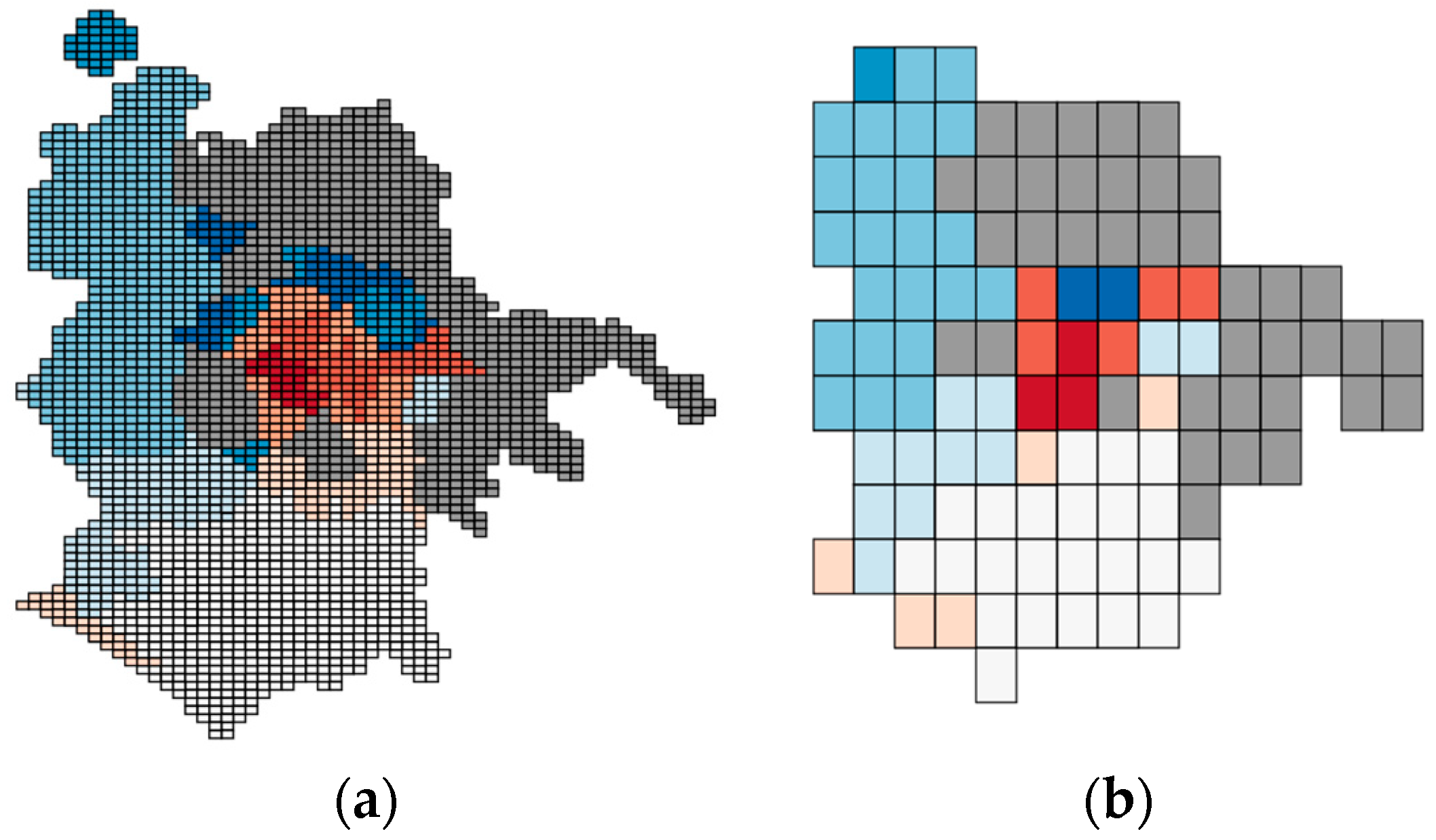
3.2.3. Geospatial Dimensionality Reduction: Geohash Encoding

Conducting large scale geospatial analytics on voluminous georeferenced data mandates two main steps. First is the data representation, which is either data-driven or space-driven, second is the access data structure. The space from which data is withdrawn is typically known as the embedding space. It can be represented as either regularly-shaped equal-sized grids or arbitrarily-shaped counterparts. Access data structures are responsible for speeding up access to target data that answers the spatial query. In summary, geospatial representation of data is succeeded by imposing a data structure on the underlying representation to boost the speed of targeted scans.

Ordering is normally assigned to cells in a grid decomposition, and thereafter a tree-based access structure (e.g., B+-tree) is imposed on the ordering. Ordering is a multidimensional reduction approach that projects multidimensional cells into a one-dimensional space. From many types of ordering, we focus on the family of z-order curves.

A special application of Z-order curves is geohash (http://geohash.org/ accessed on 10 January 2023), where the ordering imposed on the grid space is z-shaped, geocodes generated are strings where a shared prefix signifies geometrically-nearby spatial points, where longer shared prefix means objects involved are closer in real geometries. Geohash encoding is an exemplary quick-and-dirty proximity searches (i.e., working as a quick-and-dirty sieve). Figure 1a shows geohash covering generated for the city of Rome in Italy at a precision that equals 6, while Figure 1b shows the geohash covering of the same city with precision 5. Precision means the number of characters in the string representation of the geohash value. For example, ‘ws104u’ represents one of those boxes covering Rome in Figure 1a, while ‘ws104’ is the value of one of the rectangles covering the city of Rome at precision 5 as shown in Figure 1b. Longer Geohash has a granular precision (covering smaller area).

3.2.4. Spatial Query Optimization

The plain version of spatial join is expensive, which caused the introduction of optimized methods, such as filter-and-refine algorithm [39]. It operates in three steps as follows. First, spatial access methods (SAMs) are applied to restrict the search space. SAMs organize minimum bounding rectangles (MBRs) as geometric keys. It is not yielding the exact result of the spatial join, but a set of candidate pairs that contain all the answers and pairs of objects that do not fulfill the join predicate. In the second step, the candidate pairs are fed to a geometric filter that is applied to examine the pairs, for example, if the predicate is ‘contains’ then it checks the objects that are contained completely within other objects (geohash that is contained completely inside another geohash). The output is composed of three classes, true hits fulfilling the join predicate, false hits not fulfilling the predicate and remaining pairs that are possibly fulfilling the join predicate. The third step works on the exact geometry of the remaining pairs, which is expensive, and means applying ray casting algorithm (Point-in-Polygon). The filter-and-refine strategy entails a big improvement in efficiency of the inclusion spatial query. In this paper, we apply an adapted version of this approach to the execution of the spatial join between meteorological, pollution and mobility data. Figure 2 displays the workflow of the filter-and-refine algorithm (a.k.a. multi-step processing of spatial joins).

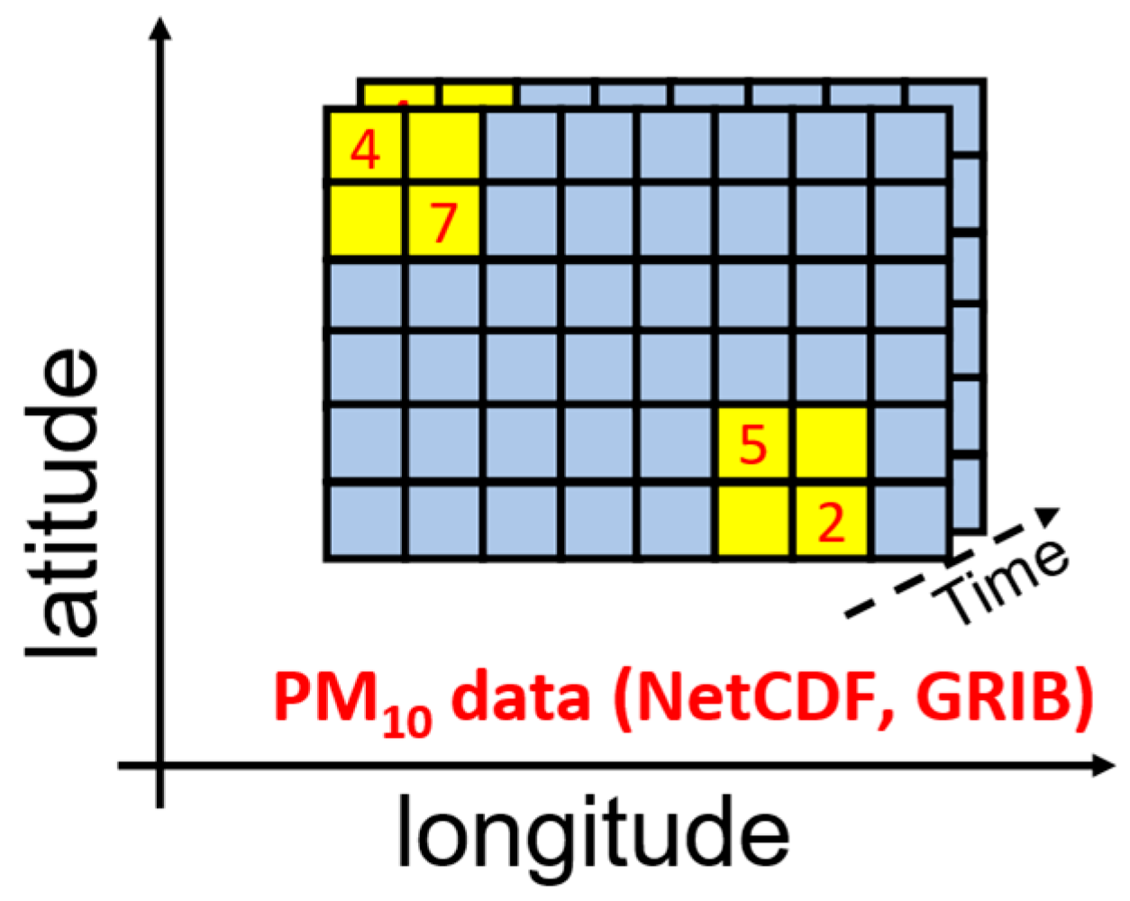
3.3. Meteorological and Pollution Data Analytics

Analyzing meteorological and pollution data is necessary for determining ecosystem evolution and analyzing patterns that may influence the future health of city dwellers. It tracks meteorological and pollution changes in a geographical context across time.

Meteorological and pollution variables captured daily by meteorological agencies include weather parameters and values such as atmospheric pressure, temperature, humidity, precipitation, solar radiation, and wind speed. Meteorological data comprise massive sources of information readily available for deep insightful analytics.

In addition to the meteorological variables, a pyramid of polluting agent’s concentrations is captured. With adverse effects of climate change and the awareness of the impact of our daily dynamics influences environment, the reduction of pollution has been a great concern for governmental bodies and people around the globe.

Air pollution includes gaseous substances that are harmful to the climate and humans alike. Among those, carbon monoxide (CO), sulfur dioxide (SO₂) and nitrogen dioxide (NO₂). Particulate Matter (PM) remains one of the most harmful forms of air pollution agents. Those are artificially and naturally created particles of thin matter suspended in the air. Those PMs have been designated as Group 1 carcinogen, as there is a direct correlation between an increase in PM concentrations and percentage rise in lung cancer incidents [40]. The numbers associated to PMs refers to the diameter of the particles in micrometers (μm); PM₁₀ particles are coarse-grained, where PM_2.5 are fine-grained.

The concentration of PM₁₀ in the area around Bologna was examined as pollution data for the scope of the project. The area, together with the rest of Northern Italy and other EU-28 urban cities have been experiencing a rise of particulate matter concentrations over the years, thus raising concerns about their adverse effect on population community health. In recent years, the lockdown attributable to COVID-19 pandemic has caused a reduction in the dust concentrations, as vehicle mobility has been restricted [41,42,43].

Meteorological and pollutions data are collected normally on two forms, Network Common Data Form (NetCDF) and GRIdded Binary or General Regularly-distributed Information in Binary (GRIB). NetCDF is an array-based representation for storing multidimensional data. A multidimensional array, having various variables with many dimensions for every variable. An example includes temperature, precipitation, or wind speed across time (a.k.a. space time-series data). It is typical in scientific data (e.g., oceanic, and atmospheric) for storing spatial time series data, for example storing meteorology and remote sensing data. GRIB on the other hand is typical in meteorology for representing weather data (historical and forecast), which is defined by the World Meteorological Organization (WMO). It is typically multidimensional files storing meteorological data in the form of sequential byte array. Figure 3 shows an example of such data.

Integrating Mobility and Meteorological Data for Joint Analytics

PM₁₀ in addition to other harmful atmosphere concentrations of substances can be integrated with human and vehicle mobility data to highlight trends and decide counteractive measures for protecting community health in urban areas. A proposed platform that aims at making this task more efficient and effortless for the end user, by providing a seamless workflow from data collection to integrated pollution, meteorological and mobility data view is depicted in Figure 4.

Thanks to the automation of technical aspects and the handling of complex tasks such as spatial joins, analysts can retrieve data from any meteorological agency (also capturing pollution data) and mobility databases, select the geographical area of interest and efficiently integrate data to find meaningful insights that assist in making strategic urban planning decisions. The provisioning of an interactive interface for querying the integrated data improves the analysis experience, allows testing sophisticated queries and exporting results to other tasks downstream a big integrated data processing workflow. In the next subsection, we discuss the details of a novel system that we have designed to realize this vision, aiming at simplifying the task of unifying and integrating heterogeneous muti-domain georeferenced data streams.

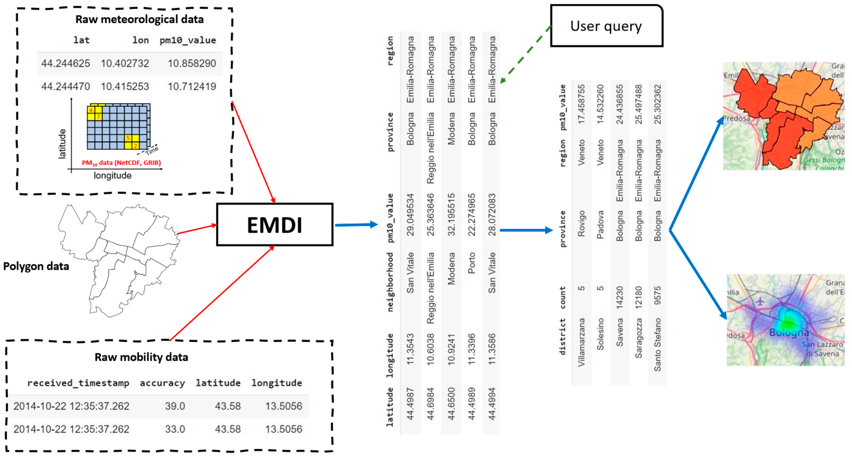
4. Mobility and Environmental Data Integration: System Overview

In this section, we show the main components that together constitute the EMDI system. Specifically, it is composed of mobility, pollution and meteorological data collector, spatial join processor and data aggregator. They work synergically to achieve a QoS processing of mobility, pollution and meteorological data combined. We first start by formulating the problem in mathematical terms.

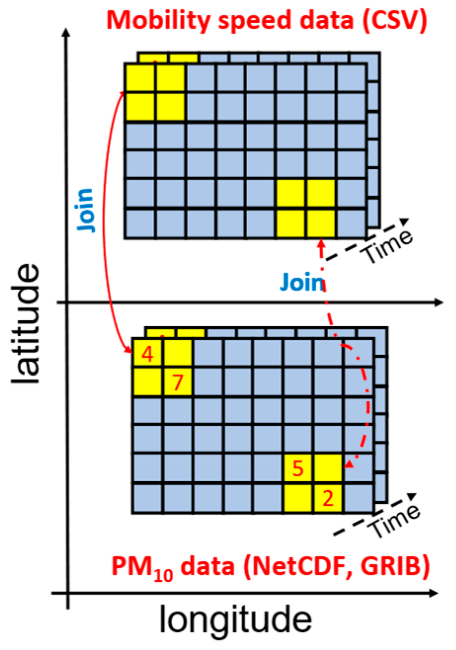
4.1. Problem Formulation

We formulate a few definitions in a sequence that assists in understanding the mechanism by which the main component of EMDI (i.e., spatial join) operates.

Definition 1. 

A georeferenced dataset S is a series that contains tuples on the form (x, y, values) such that $S=\left\{\right(x_1,y_1,v_1),\dots \dots \dots ,(x_n,y_n,v_n\left)\right\}$, where $x_i$ and $y_i$ are the geographical coordinates (typically longitudes and latitudes) of a location (point, POI, etc.) $v_i$ are some scalar values or otherwise categorical values associated with that location. For example, (x, y) could represent the location of a moving car in a trajectory, while ‘values’ represent its ‘speed’ and ‘number of riding passengers’ at that location. For pollution data, (x, y) represents the location where the measurement of the pollution level has been captured (using a fixed or moving sensing station), whereas values may represent the {PM₁₀, PM_2.5} at that location, in addition to the time the measurement was taken.

Definition 2. 

Region data R is a georeferenced data representing a geographical area (e.g., city) in the form of shapefile or a GeoJson file, where each administrative division (known as neighborhoods, districts, boroughs etc.) is known as polygon and is represented by a set of geographical coordinates on the form of $\left({xr}_1, {yr}_1, {vr}_1\right),$ such that $R=\{P_1, P_2, \dots .., P_m\}$ where $P_j=\left\{\right(x_1{r}_j, y_1{r}_j, v_1{r}_j), \left(x_2{r}_j, y_2{r}_j, v_2{r}_j\right), ........, \left(x_n{r}_j, y_n{r}_j, v_n{r}_j\right)\}$, where m is the number of polygons, n is the number of vertices (points) representing a specific polygon belonging to the region R. $x_1{r}_j$ is the x coordinate of the first point in region j.

Definition 3. 

Cross-domain plain spatial join. Given two georeferenced datasets S on the form $S=\{\left({xs}_1, {ys}_1, {vs}_1\right), \left({xs}_2, {ys}_2, {vs}_2\right), \dots \dots ., ({xs}_n, {ys}_n, {vs}_n\left)\right\}$ and $Q=\{\left({xq}_1, {yq}_1, {vq}_1\right), \left({xq}_2, {yq}_2, {vq}_2\right), \dots \dots ., ({xq}_n, {yq}_n, {vq}_n\left)\right\}$, then cross domain spatial join can be defined as S ${\bowtie }_{predicate}$ Q = {(s, q) | s $\in$ S, q $\in$ Q, $predicate$ (s, q) == true}, where a result is a series containing ‘values’ from both datasets which means S ${\bowtie }_{predicate}$ Q $=\{\left(x_1, y_1, {vs}_1, {vq}_1\right), \left(x_2, y_2, {vs}_2,{vq}_2\right), \dots \dots ., (x_n, y_n, {vs}_n,{vq}_n\left)\right\}$, where $x_i$ and $y_i$ is a longitude/latitude of a location representing both points $\left({xq}_i, {yq}_i\right)$ from Q and $\left({xs}_i, {ys}_i\right)$ from S. $predicate$ is a spatial join predicate, for example near (s, q, d) is true if ‘s’ and ‘q’ are far from each other on a maximum distance that equals to ‘d’. It is worth noticing that the join in this case is an approximation. This is so because GPS coordinates normally are inaccurate, and because we are performing the spatial join naively on the geographic coordinates, so we join from both domains (pollution and mobility in this case) based on some geometric approximation, for example the two points (the one representing pollution and the one representing mobility) are far from one another at most a predefined threshold. In this sense, this kind of join as stochastic and would never be hundred percent accurate.

Definition 4. 

Geohash-based plain filter-and-refine spatial join. It is a spatial join that is based on the plain filter-and-refine approach, where the filter stage depends on geohash encoding as the quick-and-dirty sieve. Given two geohash-enriched georeferenced datasets S on the form $S=\{\left({xs}_1, {ys}_1, {gs}_1, {vs}_1\right), \dots \dots ..,\left({xs}_n, {ys}_n, {gs}_n{, vs}_n\right)\}$, where ${gs}_1$ is the geohash value of spatial point $s_1$ in the georeferenced dataset, and $Q=\left\{{\left[\right(g_{1}r}_1, {ne}_1\right),\dots ..{(g_{m}r}_1, {ne}_1\left)\right], \dots \dots ,\dots ..[{(g_{1}r}_k, {ne}_k),\dots \dots ..,{(g_{m}r}_k, {ne}_k\left)\right] \}$ representing the covering geohash of the embedding area. It is worth noticing that every polygon in the embedding area is covered (thus represented) by several geohash values, so, ${g_{1}r}_1$ is the first geohash value covering region $r_1$ while ${g_{m}r}_1$ is the m^th geohash value covering region $r_1$, $m$ is the number of geohash values covering completely region $r_1$, ${ne}_1$ is the name of region $r_1$. Then to join mobility tuples with polygon data, the filter phase is a simple equijoin, $S \bowtie Q=L=\left\{\left(s,gs, gr, ne\right)\right|s,gs \in S, gr,ne \in Q gs==gq\}$. L is the set resulting after the refinement which is equal to the union represented by: $\bigcup _{i=1}^n(s,gs, gr, ne)$ such that within (s.x, s.y, ne) is true.

Definition 5. 

Geohash-based cross-domain filter-and-refine spatial join (the novel approach). Is an adapted, retrofitted version of Definition 4. Suppose pollution data comes in the form $p={filter}_{refine\left({pollution}_{data}\right)} \{\left({xp}_1, {yp}_1, {gp}_1, {nep}_1, {vp}_1\right), \dots \dots ., ({xp}_n, {yp}_n, {{gp}_n, {nep}_{n}vp}_n\left)\right\}$, where ${xp}_1$ is the longitude of the point in pollution data, ${yp}_1$ is the latitude of the same point, ${gp}_1$ is the geohash value representing that point, ${nep}_1$ is the neighborhood from where this point has been withdrawn, ${vp}_1$ is an array of values (pollution levels, e.g., PM₁₀ and PM_2.5) captured at that point. In addition, mobility data is represented as $M=filter\_refine\left(mobility\right)=\{\left({xm}_1, {ym}_1, {gm}_1, {nem}_1, {vm}_1\right), \dots \dots ., ({xm}_n, {ym}_n, {gm}_n, {nem}_n, {vm}_n\left)\right\}$, where ${xm}_1$ is the longitude of the point in mobility data, ${ym}_1$ is the latitude of the same point, ${gm}_1$ is the geohash value representing that point, ${nem}_1$ is the neighborhood from where this point has been withdrawn, ${vm}_1$ is an array of values (e.g., car speed) captured at that point. Then joining P and M comes down to performing an equijoin on their geohash-enriched versions such that:

$$P \bowtie M=\left\{\right(p, m, \mathit{gp}, \mathit{gm}, \mathit{nem}, \mathit{nep}, \mathit{vp},\mathit{vm}) | p \in P, m \in M, g, \mathit{ne} \in P,M gp==gm \mathrm{and} \mathit{nem} == \mathit{nep}\}.$$

The resulting set then is as follows:

$\{\left({xp}_1,{yp}_1,{gp}_1,{nep}_1,{vp}_1,{vm}_1\right),\dots \dots .,({xp}_n,{yp}_n,{{gp}_n,{nep}_{n}vp}_n,{vm}_n\left)\right\}$, containing values from both datasets that belong to the same geographical location, in this case within the same geohash and neighborhood (polygon).

In this paper, joining pollution and mobility data is an example of a cross-domain spatial join. The predicate in this case is more complicated than typical spatial join predicates, such as ‘within’, ‘touches’ etc., This is so because of the difference in the granularity (resolution) of mobility and pollution data. To the best of our knowledge, this is the first application of its kind that adapts and retrofits the plain filter-and-refinement approach for joining cross-domain georeferenced datasets with QoS guarantees. The mechanism by which we have implemented this definition in our EMDI systems is better explored in Section 4.2.

Having said that, a principal component of our system is a component that brings both datasets (mobility and pollution in this case) into the same resolution space to be able to join the two datasets. In our implementation, this resolution is represented as the geohash encoding as will be discussed shortly.

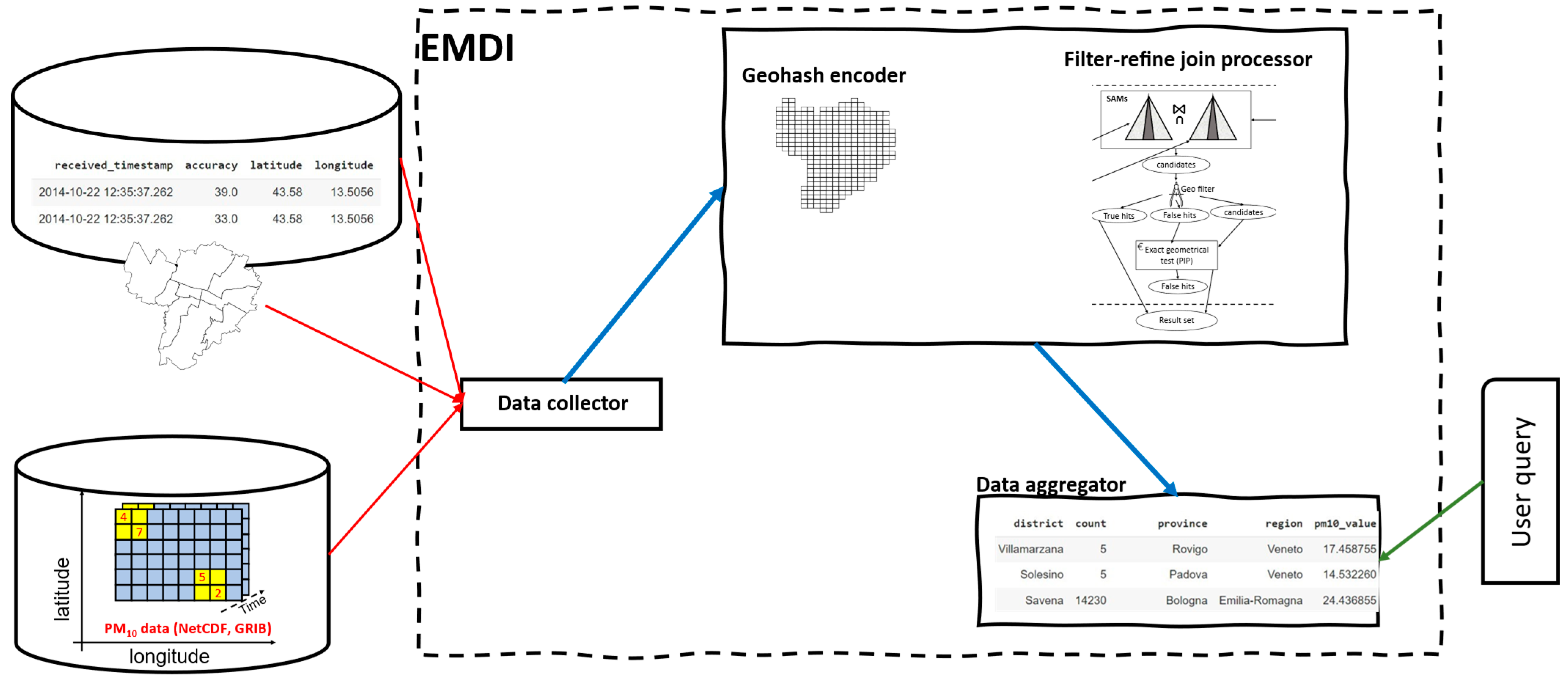
4.2. System Architecture

The architecture of the proposed system is composed of three principal components. Those are data collector, spatial join processor, and data aggregator. The system receives mobility, pollution and meteorological data and geographical maps input from corresponding online databases and websites. It then generates a unified view of the data and returns the result of a particular sophisticated spatial-oriented query submitted by the user in a tabular format that can be easily exploited for further analytics, e.g., for generating interactive region-based aggregate geo-maps such as choropleth maps and heatmaps.

From an abstract point of view, the mechanism by which EMDI system operates is depicted in Figure 5.

4.2.1. Georeferenced Data Collector

Mobility, pollution, meteorological and geographical maps data are fed from online databases and websites to the EMDI system’s data collector component. Mobility data pours as a series of Comma Separated Value (CSV) files containing a set of geographical coordinates and mobility measurements. Also, pollution and meteorological data are collected as series of NetCDF or GRIB files encompassing two-dimensional tuples of pollution and meteorological variables. It is composed of a set of geographical coordinates and a value indicating the concentration of the pollution or meteorological target variable in those locations (for example, PM₁₀ concentration). The geographical maps are represented as GeoJSON or shapefiles containing a set of polygons that represent a geographic area, from which pollution and mobility data have been captured.

This heterogeneous data is gathered automatically by the data collector. In addition to retrieving data from online sources, this component can convert pollution and meteorological GRIB and NetCDF formats into CSV counterparts for subsequent analytical tasks.

The transformations applied to GRIB and NetCDF data are executed through appropriate libraries provided over-the-counter by our system. Data integrator is also responsible for storing the output CSV files of pollution, meteorological and mobility data, and the GeoJSON/shapefiles maps in the distributed cloud storage where they can be imported by analytical engines and other analytical services.

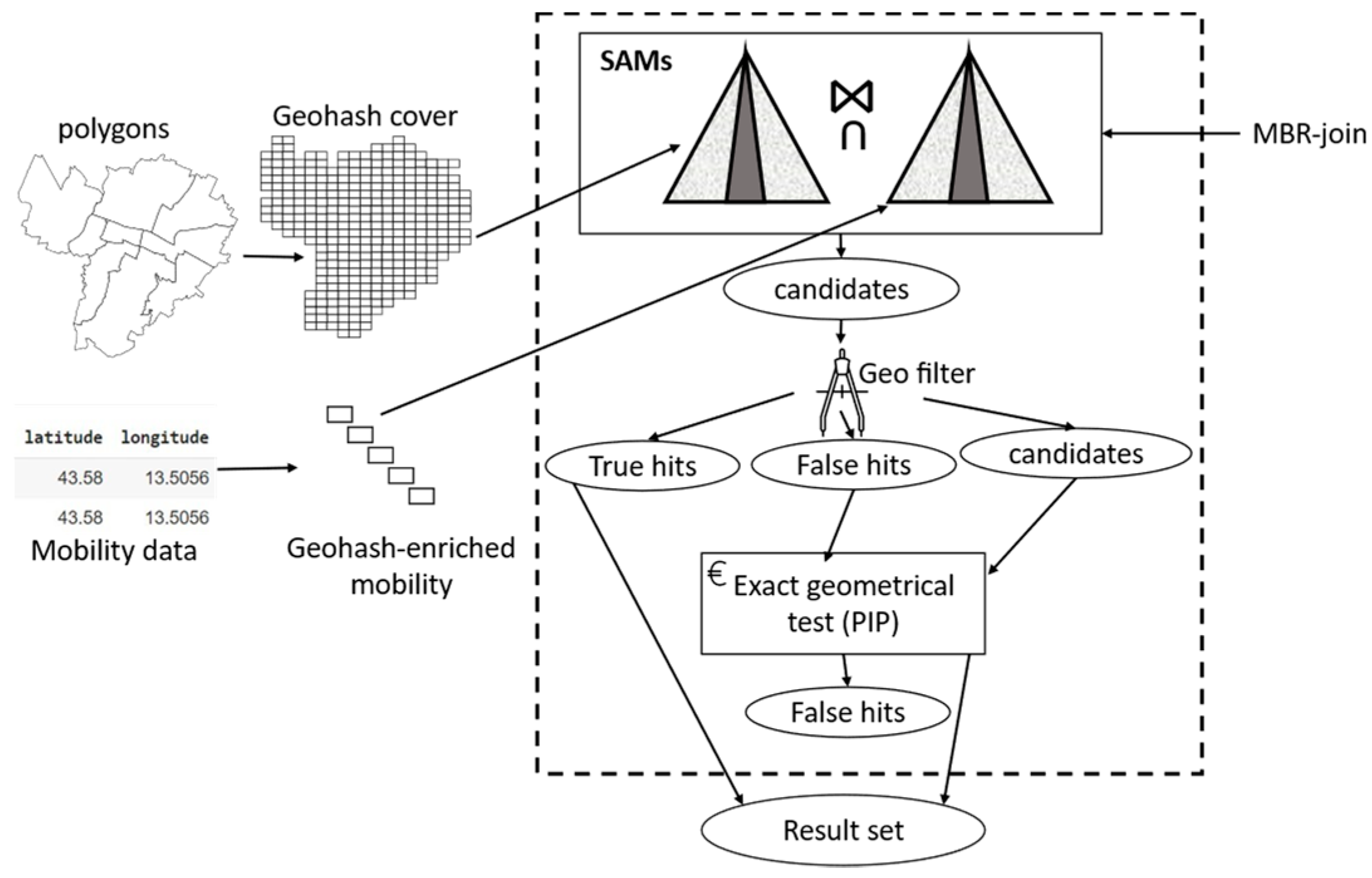
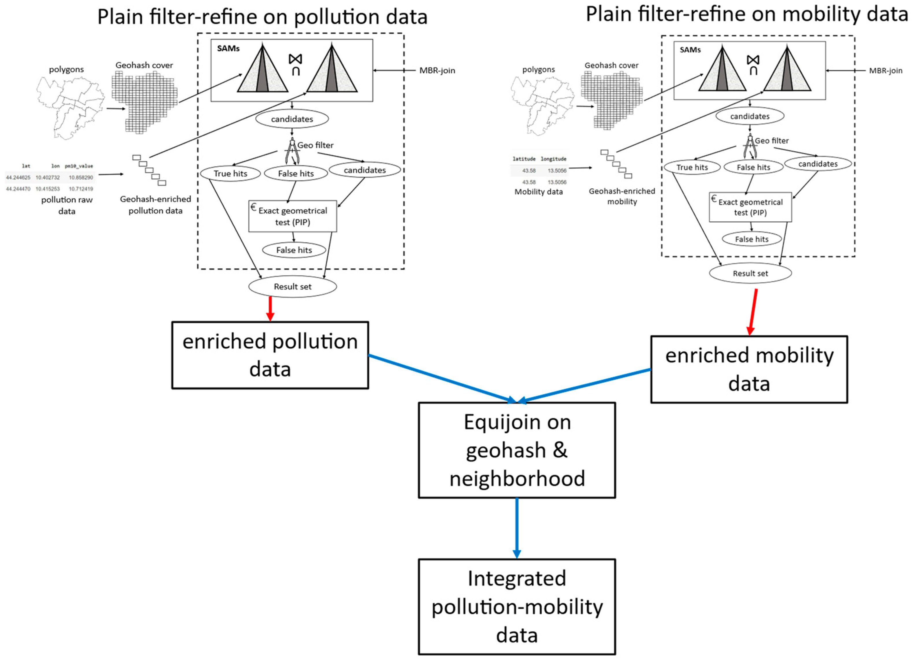
4.2.2. Spatial Join Processor

After integrated data pours downstream toward the storage, the spatial join processor starts its operation to preprocess data and put it in a unified view format. This component is divided into two logical components: geohash encoder and join processor.

The geohash encoder receives pollution, meteorological and mobility data and transforms locational coordinates information to a single-dimension string representation known as geohash. Geohash encoding accepts a pair of geographic coordinates (i.e., longitude and latitudes) and transforms them to a geometric point. Then, the component takes as input an integer that indicates the precision of geohash encoding and creates a list of Z-Order curves for referencing each geometric point. Subsequently the indexes of the Z-Order curves are hashed to base 32 and exploded from lists to single elements in each record. At the end of this process, each tuple of the datasets is enriched with a geographical location expressed as a geometric point and its relative geohash calculated with the specified precision. The geohash uniquely represents the rectangle of the grid that contains the location referenced by the point. This step is introduced for transforming the handling of geographical locations from a two-dimensional space to a one-dimensional counterpart. In this way, the spatial join comes down to an equijoin with equality conditions on string geohash representation.

The same geohash encoding is applied to pollution, meteorological and mobility data. On map data, GeoJSON/shapefiles is imported. After reading the data, the geohash encoding is applied to each polygon and a list of geohash values covering each polygon is generated as shown in Figure 6, in accordance with Definition 2 from Section 4.1.

Having the two datasets enriched with geohash codes, the system continues operation as follows. The filter step of the stock filter-refine is applied to get the pairs in three classes, true and false hits, in addition to remaining candidates. True hits are maintained, false hits are discarded, while the remaining tuples are forwarded to a refine stage that is a retrofitted, repurposed, and adapted version of the refine stage from the plain version. In the new version, each pair from the remaining candidates is checked with the exact geometry (ray casting for point and polygons in this case). This will result in two possibilities, points from mobility that fall in specific polygons and the counterparts form pollution and meteorological dataset. Then equijoin is performed to filter points that have the same geohash values and geometrically fall within the same polygon. Those are the points that will be maintained, the others will be discarded. Figure 7 shows a heuristic overview of the adapted filter-refine method, while Figure 8 shows a toy example of such join.

In summary, our join processor is an adapted, retrofitted, and repurposed version of the stock version of filter-and-refine approach. It first applies the plain filter-refine to each data with the polygon data (pollution-polygon, mobility-polygon) to enrich both data with geohashes and neighborhoods. Thereafter, it employs a simple equijoin on the two variables “geohash” and “neighborhoods” to simply join the two datasets into a unified pollution-mobility view that can be easily queried for combined sophisticated analytics. Our join processor works as per Definition 5.

4.2.3. Data Aggregator

Spatial join returns a unified view of mobility, pollution, and meteorological data, enriched with neighborhood data. This view is then fed to a data aggregator, where the newly joined dataset can be queried through user defined queries. Aggregations can be performed on the pollution and meteorological data with predicates on the mobility data and vice versa, allowing a numerous range of possible cross-domain insights to be extracted. The output of this stage is a new dataset of contextualized mobility data that can be interactively analyzed, and for which results can efficiently be exported to other services, workflow pipelines or databases. An example query can ask to “sort all city regions by highest number of mobility where PM concentrations exceed a threshold value”. This, for example, can reveal the regions with high vehicle-caused PM concentrations, i.e., those that have elevated PM concentrations caused by the excess mobility of vehicles within the city for an extended timeframe.

5. Results and Discussion

In this section, the results of performance testing of our novel system EMDI are discussed. We focus on its application with real pollution and mobility datasets and a group of queries of different computational workloads. We start with a conventional baseline with which we compare our system. Then, we discuss the details of datasets, while the last part of this section focuses on the performance tests that we performed to measure EMDI the performance of functionalities.

5.1. Baseline System

We consider a typical baseline system that performs geospatial join using a conventional method. The method requires to join tuples from pollution and mobility data at a granular scale, where geographic coordinates (longitude/latitude) of each tuple from each data set is checked against geographic coordinates of each tuple from the other dataset, resulting thus in a highly costly Cartesian product type of join. Add to this the fact that we are joining multidimensional data and the problem is exaggerated as a type of join that is better known as a Theta-join. Those types of joins require joining data on non-equal keys (longitudes and latitudes in this case). They entail high computational cost and result in very big intermediate result sets. We selected this baseline to compare with our system in terms of time-based and accuracy-based QoS constraints, such as running time and result accuracy, respectively. It is worth mentioning that the baseline system offers the utmost accuracy, but at the cost of higher computational cost, and thus an elevated latency. By selecting this baseline, we quantify the optimization provided by our system in terms of time-based QoS by abandoning only tiny statistically insignificant loss in the accuracy as discussed shortly in the results. This is so as time-based and accuracy-based QoS constraints are always contradicting in such a way that optimizing one of them tampers with the other. So, finding a balance between them both should be the target, which is one of the main contributions of this paper.

5.2. Deployment Settings

5.2.1. Datasets

To test the efficiency and capabilities of EMDI, we employ two types of georeferenced datasets to represent pollution and mobility data. The pollution datasets selected for the demonstration are aimed at showing the capability of the system in accepting the two most widespread formats, GRIB and NetCDF.

The files received in the two formats are transformed into the standard CSV format that is accepted by big data analytics frameworks.

Table 1. Datasets with number of tuples and main attributes.

Datasets	Size (Tuples)	Attributes
Mobility (Bologna)	500k	lat, lon, timestamp, trip_value
Meteorological (Bologna)	66k	lat, lon, pm10_value, timestamp
Neighborhoods (Bologna)	9	Polygon, city, region, province

shows the characteristics of the datasets employed, the type of data, the size in tuples and the main attributes included.

• Meteorological and pollution data

The first meteorological dataset is the CAMS (for Copernicus Atmosphere Monitoring Service) global reanalysis (EAC4) data coming from the Atmospheric Data Store (ADS) of ECMWF (for European Centre for Medium-Range Weather Forecasts).

The reanalysis works on data assimilation principle, through which previously captured forecasts are integrated with newly available observations to produce a relevant estimation of the atmosphere conditions across time. The data points of the EAC4 reanalysis are set on an 80 (km)-spaced grid across the globe. The dataset employed in this paper is the PM₁₀ (for Particulate matter d < 10 µm) concentrations, with records taken on a time distance equals roughly to 3-hourly from “00:00” to “21:00”.

We selected a rectangle that roughly incorporates the territory of Italy as the covered study area for the data. To do so, we join georeferenced mobility data with neighborhoods (i.e., polygon) data of municipalities in Italy, we then extract minimum and maximum latitude/longitude values from the resulting dataset.

We extracted data for a time interval that roughly equals to one month in 2014 to match the corresponding time interval in the mobility data. This results in 3-h-spaced tuples for the bounding rectangle covering Italy, which amounted to circa 21,500 tuples.

From the resulting dataset, we selected latitude/longitude coordinates, the timestamps, in addition to the target variable, specifically the concentration of PM₁₀ in the 3 h span measured in kg/m⁻³.

The file format for this pollution data source is GRIB, downloaded through the ADS API and transformed into CSV by the data collector component of the EMDI system.

We capture the second meteorological dataset from the analysis of Urban SIS (Sectoral Information System) [44], a demonstrator project that aims at developing, demonstrating and testing a method to downscale climate indicators to an urban scale (specifically a grid size of roughly 1 km²) for practical smart city applications. The dataset contains daily concentrations of PM₁₀ pollutant in major cities of Bologna, Modena, Reggio Emilia, and Ferrara in Italy. The file format for this dataset is NetCDF, which is then transformed into CSV by our data collector.

From this dataset, we extract latitude/longitude coordinates together with the target value. The target value includes the 90th percentile concentration of PM₁₀ of daily averages for one year. Values are measured in µg/m⁻³ and limited to maximum 50 µg/m⁻³; a value that is imposed by the European Union.

All the datasets were imported as a CSV file format using Jupyter notebooks and the latitude/longitude coordinates were transformed into geospatial data structures.

2.

Mobility data

The mobility dataset comes from the ParticipAct [45,46,47] project of the University of Bologna. ParticipAct gathers data on a large scale with the contribution of students at the University of Bologna and volunteers through a smartphone application that allows the coordinated collection of selected data. The aim of the project is to study the potential of collaboration among people exploiting smartphones as an interaction tool and interconnection medium.

From the ParticipAct project we retrieved four datasets of different sizes to be used as part of our tests. Datasets were labelled with their approximate length of records as 20k, 100k, 250k and 500k records. We selected a subset containing 500k tuples, reporting data spanning one month of the year 2014.

The data was received directly in CSV format from the source, hence no transformation pre-ingestion in the spatial join processor was required. Attributes include record id, timestamp at which the data was captured, measurement accuracy, latitude and longitude coordinates, data provider, user id of the of the device collecting the data and timestamp of the sample gathered.

5.2.2. Deployment Settings

We deploy our experiments on VM that runs on Google Collaboratory with 13 GB RAM and 2 vCPU (2 Intel(R) Xeon(R) CPU @ 2.20 GHz).

5.3. Testing Scenarios

In this section, the various types of tests that we run to present the EMDI system capabilities are discussed. We run different kinds of standard spatial queries that can be used as benchmarks to measure the performance of the system in different scenario workloads.

5.3.1. Queries Supported

In this subsection, we describe the queries supported by our EMDI system on the unified views generated for pollution and mobility data.

• Top-N query

To measure the potential of our EMDI system in handling complex combined analytics of pollution, meteorological and mobility data, we tested it on a top-N kind of geospatial queries, such that we retrieve sorted counts of mobility data with predicates on location and pollution data dimensions. Specifically, we tested with the following query: “what are the top-N neighbourhoods in Bologna in Italy in terms of the amount of human mobility density where the PM₁₀ concentrations are greater than or equal to a threshold, e.g., 24?”. We computationally stress the system with this kind of queries. This is an aggregation type of query that involves grouping and sorting by city regions in addition to the cross-domain spatial join and count upstream.

2.

Average query

Specifically, we tested the following query: “what is the average value of PM₁₀ concentration per neighbourhood in regions affected by PM₁₀ value that exceeds a threshold, e.g., 24?”. With this query, we test the EMDI system’s ability to answer single geo-statistical queries such as ‘mean’.

5.3.2. Significance of the Performance Tests

Queries discussed in the previous section are designed to be generic enough to demonstrate the versatility of our EMDI architecture. Those queries are non-trivial and computationally expensive enough to render the testing scenarios realistic, especially with heterogeneous datasets that are relatively big.

By performing those tests, we aimed at showcasing a range of capabilities that are novel in the field of joint mobility, pollution, and meteorological data analytics. With the EMDI system, we introduce a tool to integrate pollution, meteorological and mobility data, to generate a unified view for combined analytics. The aim of the two tests is precise and well-defined to test the skills of our EMDI system in real settings.

Specifically, for the geospatial geo-statistical ‘average’ test, we calculate average PM₁₀ values by districts where the pollutant concentration levels are higher than a specific threshold. This kind of queries is very relevant for urban planning and decision making, and we have designed EMDI in such a way that those single geo-statistical queries can be executed by varying the level of granularity so that we can calculate at coarser level of provinces and regions, thus varying the granularity level of aggregation between granular and coarser. Consequently, this can reveal the way the concentrations of PM₁₀ pollutants influence human mobility on a granular or coarser scale, thus highlighting micro and macro patterns of human urban mobility, respectively.

For Top-N queries, we tested the possibility to rank municipalities which have the highest levels of human mobility and high levels of PM₁₀ simultaneously. This kind of queries, which requires ranking cities (or districts within a city at a granular level of details) and discarding municipalities with pollutants concentrations that are below a certain threshold, wouldn’t be possible without integrating pollution and mobility data within the same data view. This is so because in this kind of queries, we are counting mobility data in each district with a predicate that is imposed on pollution data, thus contextualizing mobility data with pollution data tags.

Such an application scenario is interesting for city planners and decision makers in metropolitan cities because they may need to check relationships between PM₁₀ concentrations and mobility of city dwellers and vehicles circulating within their cities. This is beneficial, for example, to enforce mobility policies that help them to adhere to national or international regulations regarding allowed pollution levels in major metropolitan cities.

In the same vein, other types of more complicated queries are thus constructable from those baselines queries. For instance, trajectory queries such as “finding out whether people walk less in certain areas of a city or a street because of high PM₁₀ concentration”, which could be unintentional without prior knowledge, but simply feeling unwell by commuting regularly in those areas with high pollution levels. Also, queries such as “is there a correlation between people using their cars rather than walking in a certain area and high concentration of polluting substances”. Those kinds of queries can be answered by our system by simply gathering granular data instead of designing a new domain-specific system.

By technologically abstracting optimization layers such as spatial join inner logistics handling to decision makers and front-end developers and enabling a seamless querying of integrated pollution and mobility data through a simplified interface, we provide an added novel value that is offered by our system.

5.4. Testing Procedure

In this section we describe the testing procedure that we applied to run the set of queries described in Section 5.3.1. We also discuss various configuration settings that we varied to outline to showcase the performance of our system.

5.4.1. Variation of Data Loads and Query Types

We first vary workloads by running various queries described in Section 5.3.1, and capture the queries running times, including time imposed by the cost of creating the unified view. To account for machines stochastic behaviours, we repeat the queries tests 10 times and captured the 95th percentile of the measurements to delineate an accurate measure of the system’s query run times.

We specifically vary the size of mobility data to understand system behaviours with varying data load, specifically we vary loads with the following: 20k, 100k, 250k and 500k tuples.

For the brute-force baseline, we measure the total running time as in Equation (2).

Total running time for baseline = tb1 + tb2 + tb3.

(2)

where tb1 is the time required to brute-force join mobility data with the neighbourhoods represented in polygons, tb2 the time required to brute-force join pollution data with the neighbourhoods represented in polygons, tb3 is the time required to perform the Cartesian product join between the two intermediate datasets, thus ultimately generating the unified view.

As a way of contrast, we measure the running time for our novel system EMDI as in Equation (3).

Time for EMDI = te1 + te2 + te3 + te4.

(3)

where te1 is the time required for applying the filter-refine to join mobility data with polygons, whereas te2 is the time required for applying the filter-refine to join pollution data with polygons, te3 is the time required to calculate the sketches for the pollution data, te4 is the time required to perform the equijoin on the resulting intermediate datasets.

5.4.2. Testing Accuracy

While the baseline brute-force method offers the finest accuracy due to its design, it entails higher computational cost. We trade-off higher gain in latency for tiny negligible loss in accuracy.

For Top-N queries, which are stateful aggregations, we apply two correlation coefficient measurements, Spearman correlation coefficient [48] (a.k.a. Spearman’s rho) and Pearson correlation coefficient. Using those measurement tools from the information theory, we measure the accuracy in terms of the method’s ability in preserving the aggregation’s original ranking. Spearman’s rho is a measure for statistical dependency between the ranking of two variables in a dataset. We have adapted and retrofitted those measurements as follows: We take the ranking that results from each method (our EMDI method against the baseline), then we serve those to the plain Spearman’s rho, and we apply Equation (4).

$${\mathsf{\rho }}_{\mathrm{rg}}=\mathrm{cov}({\mathrm{rank}}_{\mathrm{EMDI}}, {\mathrm{rank}}_{\mathrm{baseline}}) / ({\mathsf{\sigma }}_{{\mathrm{rank}}_{\mathrm{EMDI}}}·{\mathsf{\sigma }}_{{\mathrm{rank}}_{\mathrm{baseline}}}).$$

(4)

where ${\mathsf{\rho }}_{\mathrm{rg}}$(pronounced rho) is spearman’s correlation coefficient applied for ranking statistics, $\mathrm{cov}({\mathrm{rank}}_{\mathrm{nos}}, {\mathrm{rank}}_{\mathrm{samp}})$ is the covariance of the rank variables, ${\mathsf{\sigma }}_{{\mathrm{rank}}_{\mathrm{EMDI}}} \mathrm{and} {\mathsf{\sigma }}_{{\mathrm{rank}}_{\mathrm{baseline}}}$ are the standard deviations of the rank variables for EMDI and baseline, respectively.

Pearson correlation coefficient (PCC for short) is another important tool from the information theory. It basically measures linear correlation between two data distributions. It is simply calculated as the ratio between the covariance of the two variables and the product of their standard deviations. In this sense, it is considered as a normalized measurement of the covariance. The outcome is a value between −1 and 1. It is calculated as in Equation (5).

$${\mathsf{\rho }}_{\mathrm{E}\mathrm{M}\mathrm{D}\mathrm{I},\mathrm{b}\mathrm{a}\mathrm{s}\mathrm{e}\mathrm{l}\mathrm{i}\mathrm{n}\mathrm{e}}=\mathrm{c}\mathrm{o}\mathrm{v}(\mathrm{E}\mathrm{M}\mathrm{D}\mathrm{I},\mathrm{b}\mathrm{a}\mathrm{s}\mathrm{e}\mathrm{l}\mathrm{i}\mathrm{n}\mathrm{e})/({\mathsf{\sigma }}_{\mathrm{E}\mathrm{M}\mathrm{D}\mathrm{I}}·{\mathsf{\sigma }}_{\mathrm{b}\mathrm{a}\mathrm{s}\mathrm{e}\mathrm{l}\mathrm{i}\mathrm{n}\mathrm{e}}).$$

(5)

The difference between both correlation measurements is that PCC assesses the linear relationship between variables, whereas the Spearman correlation coefficient evaluates the monotonic relationship.

For testing accuracy of average queries, we applied Mean Absolute Percentage Error (MAPE), which is a measure of prediction accuracy, and is calculated as in Equation (6).

$$MAPE=\raisebox{1ex}{$100\%$}\!\left/ \!\raisebox{-1ex}{$n$}\right. {\sum }_{i=1}^n\left|\raisebox{1ex}{$A_i-F_i$}\!\left/ \!\raisebox{-1ex}{$A_i$}\right.\right|.$$

(6)

where $A_i$ is the actual average value calculated form the unified view that results from the baseline method, whereas $F_i$ is the average value calculated by our EMDI method. n is the number of times we repeat the test to account for stochasticity nature of the calculation.

6. Results Discussion

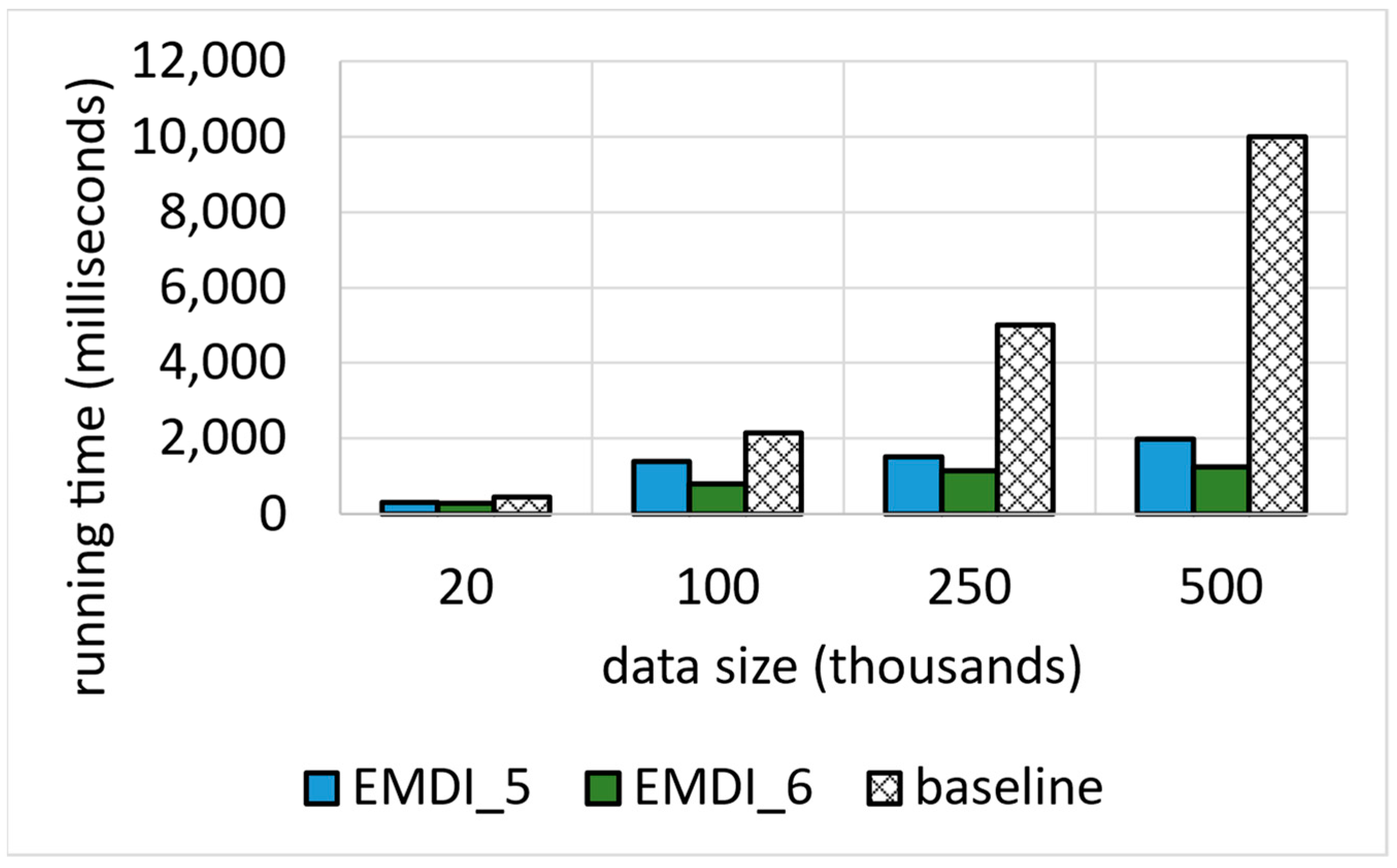
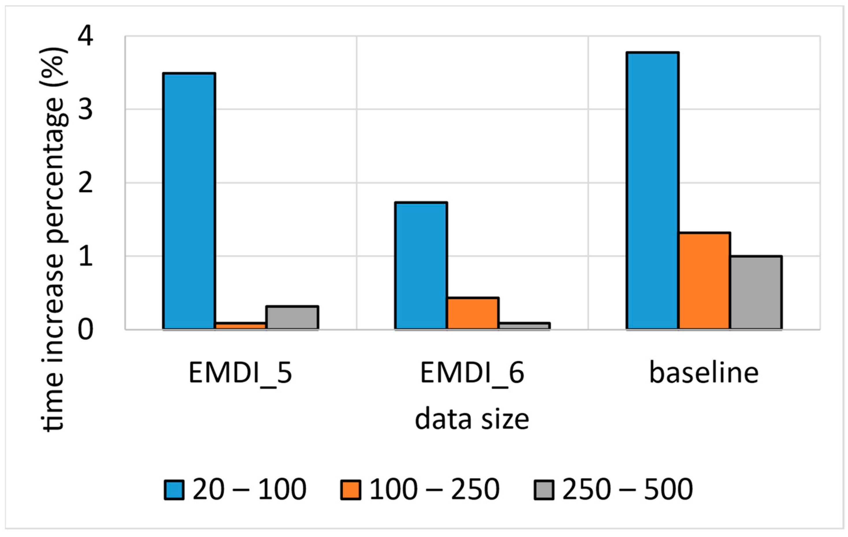
In this section, we show the results of the performance testing scenarios highlighted previously.

6.1. Running Time

Figure 9 shows the results of running times for Top-N queries performance tests as calculated using Equations (2) and (3). The running time increases linearly with the increase in size of input mobility data for all methods including our EMDI method (with varying geohash values) and the baseline.

It is obvious that a lower geohash value entails a higher computational cost, and consequently an elevated running time. Our explanation for this is the following. Lower geohash precision means a bigger area coverage for each geohash value, this means that more points from both datasets will have same geohash values and belong to same geohash brackets. This has a direct impact on the spatial join operations, being it the baseline cross join or even the equijoin part of our EMDI method. In other terms, more tuples from both datasets will match, resulting thus in a bigger result set and join processing times.

Latency grows slowly and linearly with the increment of the input dataset size. The increase of input dataset size is in the orders of 500%, 150%, 100%, respectively, meanwhile the growth in latency is shown in Figure 10. We can notice that the growth in running time for EMDI with geohash precision 6 is the lowest among all. For the baseline it grows exponentially with the increase of the data size on the orders discussed previously. We can conclude that geohash precision 6 is a reasonable and best choice value in this case.

As shown in Figure 10, the running time of top-N tests, for EMDI with both geohash precisions against the baseline. It is obvious that the running time for the baseline is much bigger than our new system EMDI. This is so because Top-N for the baseline needs to perform more aggregation based on the neighborhoods than those of the EMDI system. The fact that for the EMDI system we draw sketches from the pollution data reduces the result set for which the Top-N need to be performed with.

The picture that emerges is the following, we are satisfied with the latency and execution times of the EMDI system as compared to the baseline. We did not observe any exponential growth in this case, as running time growth will become linear and stabilize after reaching a certain input size.

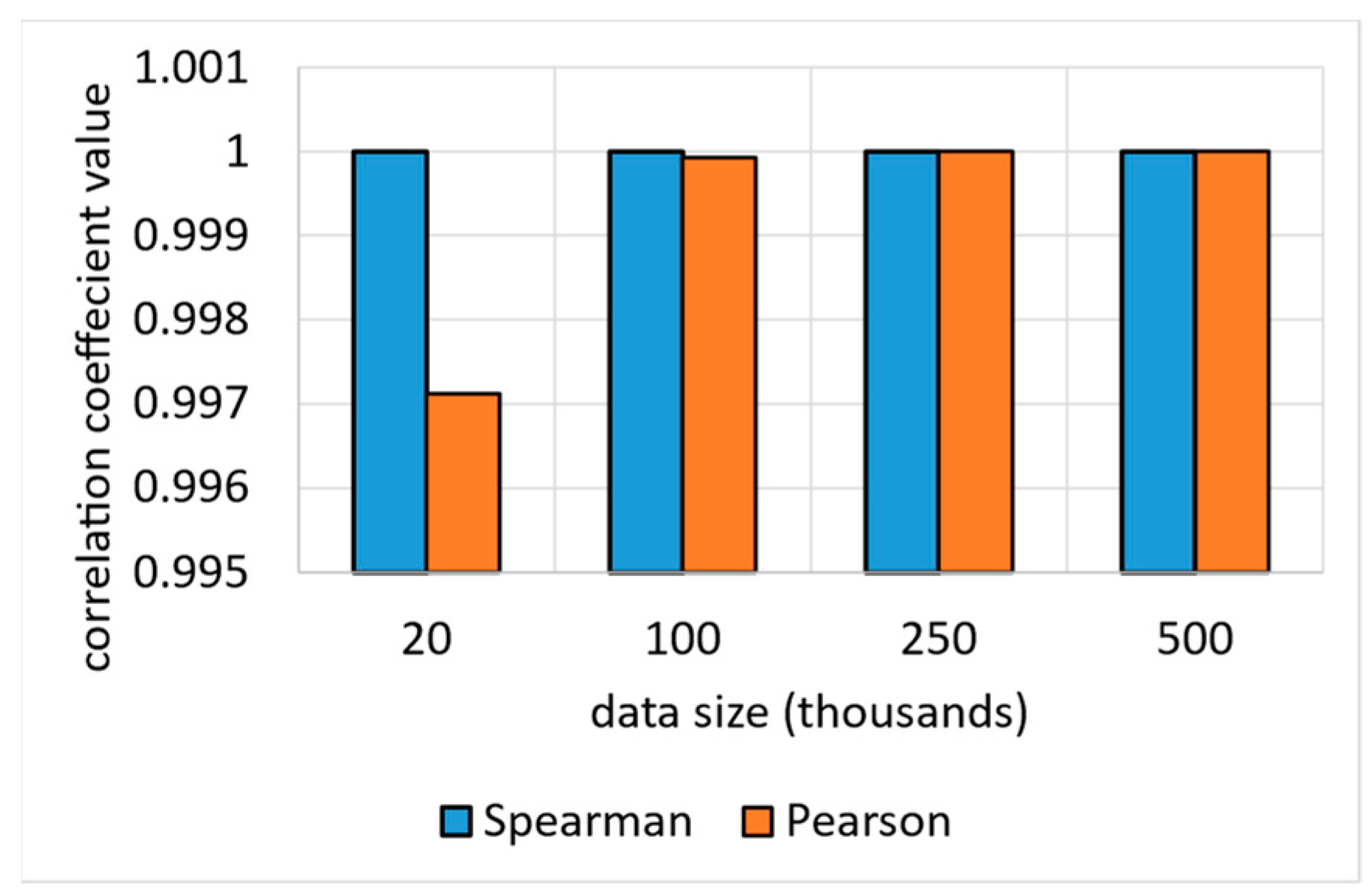
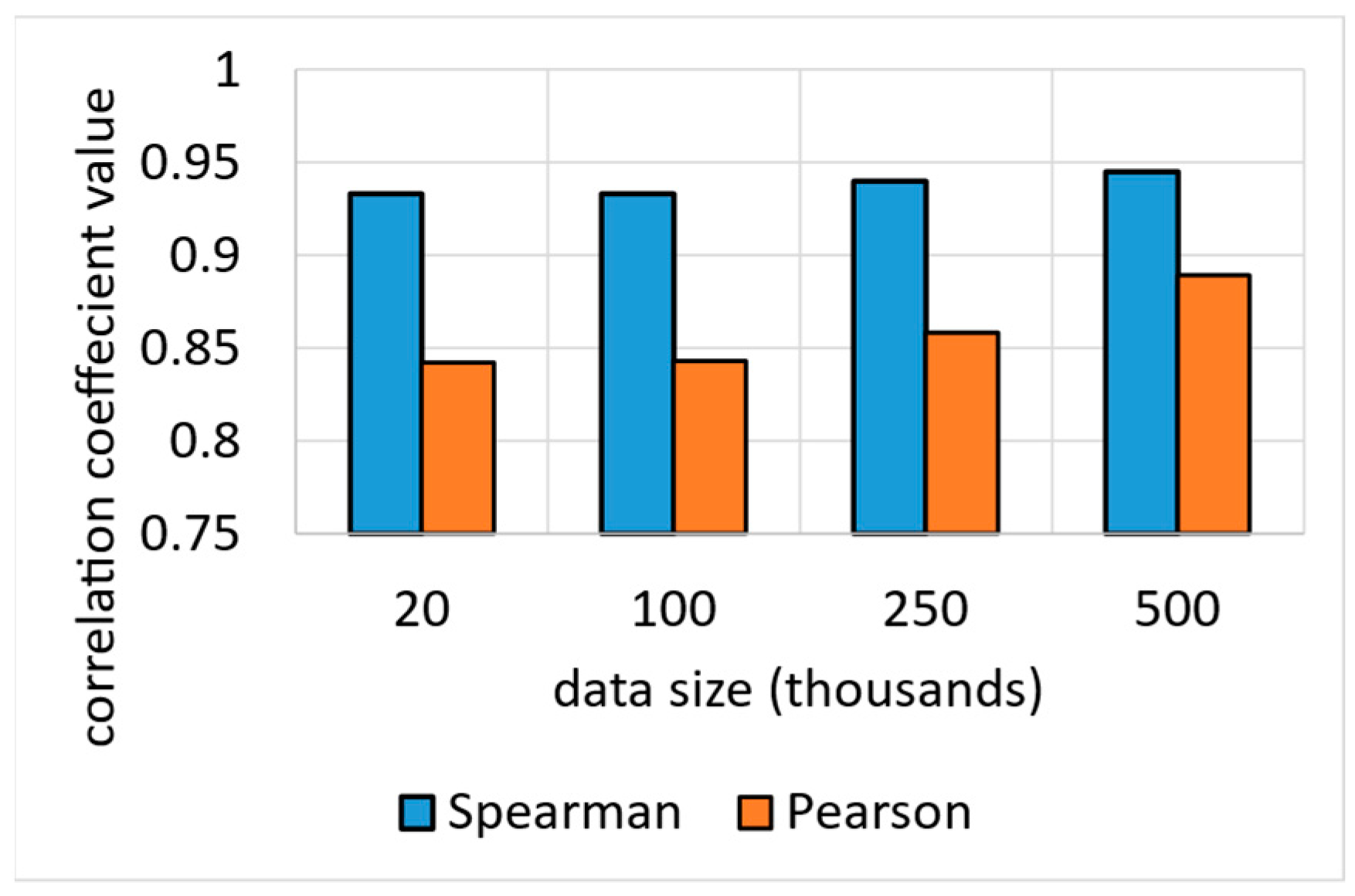
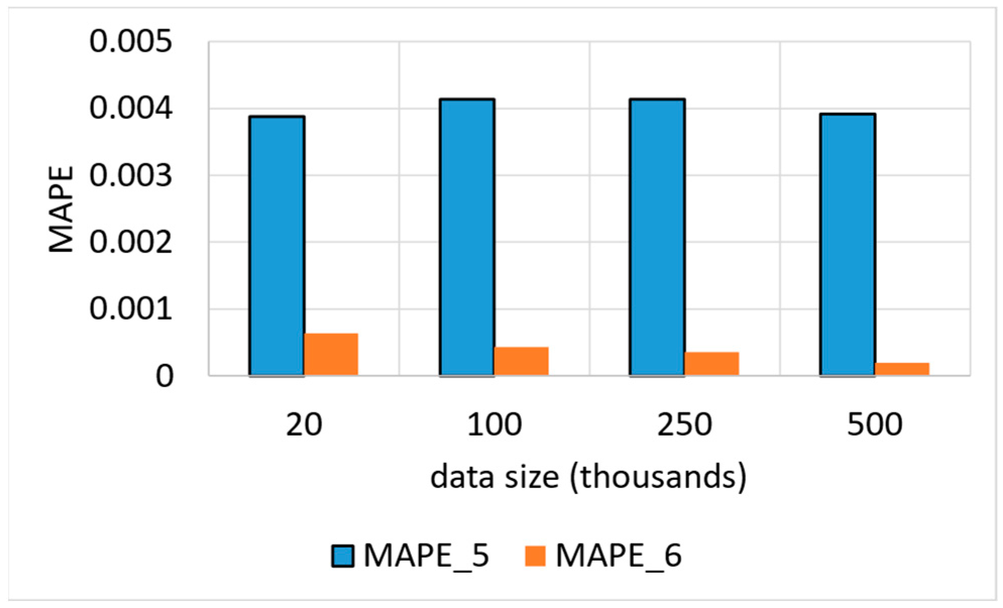
6.2. Accuracy Test Results

Figure 11 shows the test results of the accuracy performance of our EMDI system for Top-N queries. Both correlation coefficients PCC and Spearman’s rho, show a statistically significant relationship, with values for Spearman’s rho ranging from roughly 0.9999 for data size that equals to 20k tuples, to around 1 for data size that equals to 500k tuples. Those are the figures for granular geohash precision that equals to 6. Similar results obtained for the PCC, despite being slightly lower than the Spearman’s, however, remain statistically significant. Comparatively speaking, for a coarser geohash precision, specifically a value that is equal to 5, the figures are lower, with PCC ranging from roughly 0.84 for data size that equals to 20k tuples, to around 0.89 for data size that equals to 500k tuples, still statistically significant despite that we obtain better numbers for the Spearman’s rho as shown in Figure 12.

It is obvious that we obtain higher accuracy for the Top-N queries by applying geohash precision 6 instead of 5 as shown in Figure 12.

This is very significant as we have noticed that increasing the geohash precision will increase the correlation coefficient values (Spearman’s rho and PCC). This is so because by increasing the geohash precision we are working on a granular level, which means we are considering more geohash values for the same geographic areas, and subsequently means granular, and more accuracy is achieved because we depend on grouping by geohash values for the PM₁₀ observations and then joining the grouped result with the mobility data. This means a higher join cost should be involved; however, more accuracy is obtained.

For the average queries, we show the results of testing using MAPE as discussed in Section 5.4.2 Specifically, we apply Equation (6). Again, we vary the data size and the geohash precisions. Results obtained are shown in Figure 13.

We notice that the higher the geohash precision the lower the value of MAPE, which is desirable.

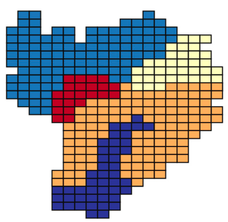
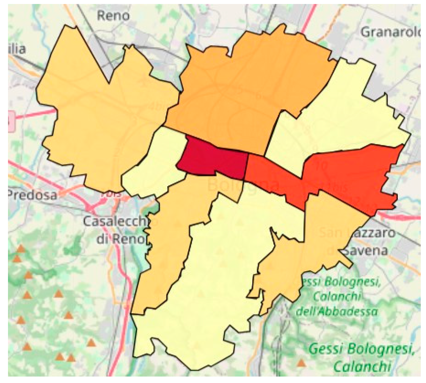
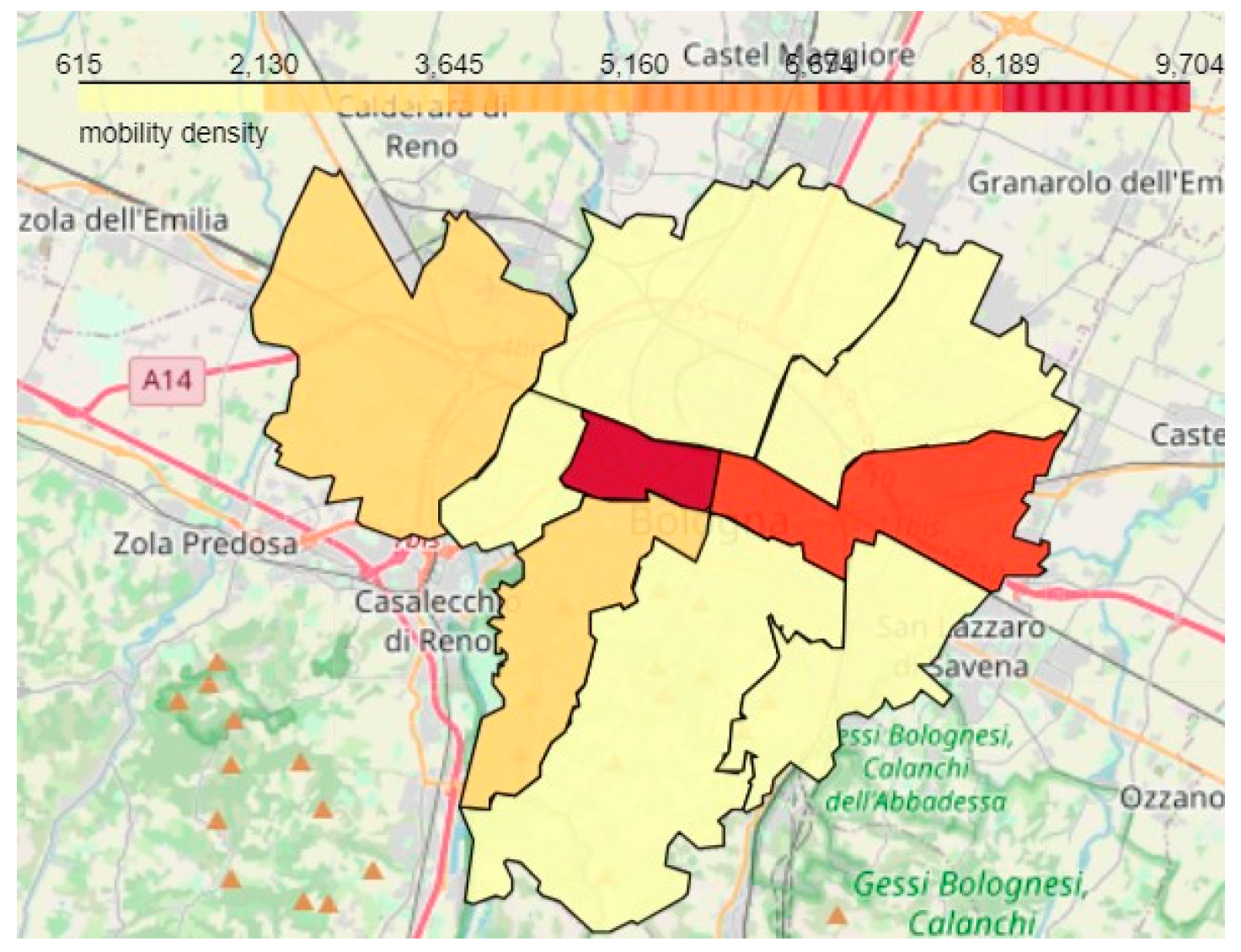
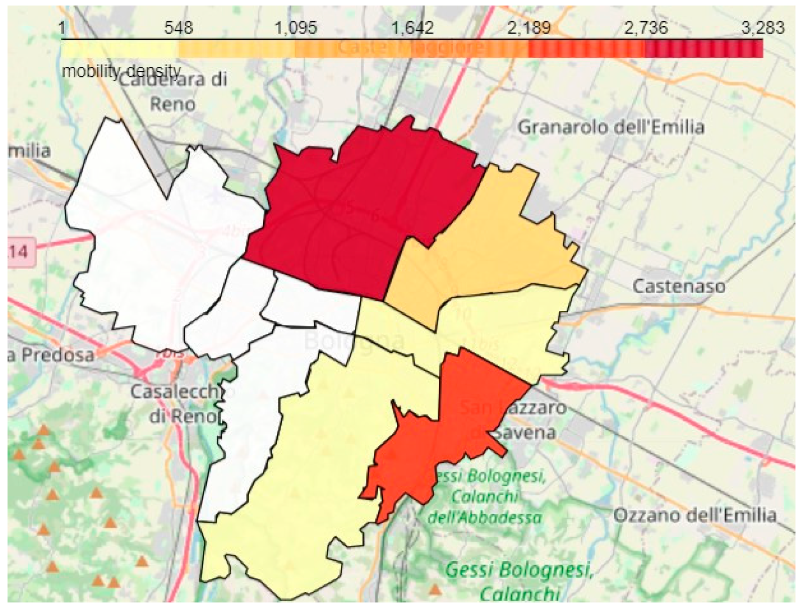
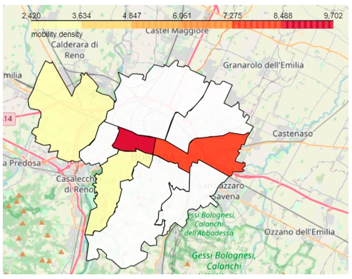
6.3. Testing the Ability to Generate Region-Based Aggregate Geo-Maps from the Unified View

In this test, we aim at testing the ability of the EMDI system to generate sophisticated region-based aggregate geo-maps (such as choropleth maps) based on conditions and predicates imposed on a unified view representing mobility and pollution data.

Specifically, the following query, “retrieve the Top-N neighborhoods in Bologna in Italy in terms of the density of dwellers mobility who are potentially exposed to PM₁₀ substances on a concentration that exceeds a given threshold ‘say 24.5 for example’”. By using our system, we could easily, with a click of a button, generate such a map, thanks to the integrated view of mobility-pollution data generated previously by our adapted filter-and-refine spatial join method as an integral part of our EMDI system. Figure 14 shows original density in correlation with PM₁₀ at all levels, whereas Figure 15 shows the resulting map. As can be seen, where PM₁₀ is less than or equals roughly to 24.5, Figure 16 reveals the density of dwellers exposed to such levels.

Figure 17 shows an example on a predicate applied to pollution PM₁₀ ≥ 24.5, where density of commuters is greater than 2k. The figures show that most affected areas are near the airport and near the city center.

One can then choose to apply spatial-aware distance tools from the information theory such as Earth Mover’s Distance (EMD) [49] to quantify the dissimilarities between maps and generate conclusions in terms of the correlation between the density of dwellers and their exposure to PM₁₀ elevated numbers.

7. Challenges and Future Research Perspectives

A challenge that is typically encountered is the availability of data. Also, the data being it meteorological, pollution or mobility data have some issues with either spatial or temporal coverage. Other challenges include the fact that mobility and pollution data come in different formats. Mobility data comes in tabular (e.g., CSV) and georeferenced meteorological and pollution data in NetCDF or GRIB formats. Selecting the right data from a constellation of heterogeneous sources adds to the challenge, also GPS data is not 100% accurate, and there is a loss of accuracy during data collection, hence GPS coordinates can be inaccurate when the handset is moving quickly, such as in a car or airplane. In addition, meteorological and pollution data may have been collected with differing sets of spatial granularities (granular & coarser). In this case, interoperability is key, where spatial interoperability means that data matches up in the spatial dimension. On the other hand, temporal interoperability means that meteorological, pollution and mobility data match up in temporal space. Other questions may arise, including the following scenario, imagine the earth flattened and gridded, what is the size of each grid cell for which meteorological or pollution data is aggregated? What distributed data management methods can be used to store and process such georeferenced multidomain data, at scale? Also, talking about spatial resolution, “what is the smallest unit of area measured?”, We obtain a lower resolution by aggregating the data over a greater area, which makes it more difficult to reason about the data on a smaller scale. Also, answering whether there had been an increasing median PM₁₀ caused by vehicles density on a granular level. It would then be hard to establish the pattern, considering that mobility resolution is substantially lower than meteorological and pollution data resolution. Changes of median vehicle density in other parts of the coarser resolution might obscure or falsely enhance what is happening on granular level. Moreover, considering temporal resolution, the frequency at which spatial data has been collected, and how often the measurements are taken, as we may collect mobility data daily, whereas meteorological and pollution data is taken every few hours for the same geography. It is not easy to discover the correlation between mobility, pollution, and meteorological data on an hourly basis, based on different temporal resolutions.

As a future research perspective, we consider adding support for new spatial queries. We currently support single geo-statistical queries that return single values, such as ‘count’ and ‘mean’. In addition, we support aggregation spatial queries, including Top-N. Moreover, we support geo-visualization in the form of region-based aggregate geo-maps such as heatmaps and choropleth maps. All those queries are supported on predefined set of geometries with extents, i.e., administrative regions division of a city in the form of irregularly-sized polygons served to the system in the form of GeoJson or shapefiles, together with the other data sources. Proximity queries are potential candidates. Those require defining customized regions of search within the study area. For example, “what are the nearest 5 Points-of-Interest (POIs) to my current location with a radius less than 10 km and a PM₁₀ average value less than 11”.

Also, trajectory analytics support can be added to the EMDI system by plugging functionalities provided by other systems such as scikit-mobility [50]. It would then be possible to develop an interactive map for daily dwellers in metropolitan highly-polluted cities, such as to show the ‘green paths’ where those dwellers and cyclers can practice sport without being exposed to high levels of detrimental substances such as PM₁₀. Also, municipalities can use those statistics to decide the locations of new schools and green parks based on such data analytics.

In this paper, we have considered the average PM₁₀ in each geohash to generate sketches for geohash values to serve a reduced pollution dataset for the subsequent join step with the mobility data (which was an equijoin). In the future otherwise, we would consider other possibilities by considering more robust statistical analysis within the values for each geohash to select the method with which we draw sketches deeply grounded on information theory. For example, we could take the ‘mean’ value from some geohash brackets, while taking the maximum and minimum from other brackets depending on those statistics. We corroborate that this would result in more accurate results. However, we have selected the ‘mean’ statistic in this paper as our statistical analysis for this data shows that it is normally distributed (bill-shaped) for the mean PM₁₀ values for all locations (geohashes) meaning that PM₁₀ values are clustered around the true PM₁₀ mean with 68, 98,99.7 confidence intervals rule applies in this case.

8. Conclusions

The EMDI system is a novel architecture that allows the interactive integration of pollution, meteorological and mobility data at scale with QoS guarantees. Our system guarantees a statistically significant balance between time-based QoS metrics (end-end latency as discussed in Section 6.1) and quality metrics (depending on the query, either high correlation coefficient value for Top-N queries or low MAPE value for single statistics such as ‘mean’) as discussed in Section 6.2. To recapitulate and summarize the supporting results, our system lowers the latency (a desired time-based QoS constraints) by approximately 65% and achieves a high accuracy (desired quality-based QoS constraint) as opposed to the plain baseline, as we obtain an accuracy for Top-N queries that ranges from 0.84 to 1 for Spearman and Pearson correlation coefficients, values that rely on the geo-encoding configurations. Also, for single geos-stat queries (such as ‘mean’), we obtain MAPE values ranging from roughly 0.00392 to 0.000195, which is statistically significant. The novel aspect of this architecture is the application of an adapted, retrofitted, and repurposed version of the filter-and-refine algorithm for performing the spatial join, which reduces the execution times that would otherwise be computationally expensive.

Our architecture is composed of three main components: data collector, spatial join processor and data aggregator. The first component retrieves neighborhood, pollution, and mobility data from publicly accessible online databases. It also applies the required data transformations. The second component executes spatial joins and transformations with the application of Z-order curves geohash encoding and retrofitted filter-and-refine algorithms, thus speeding up the process. Data aggregator component provides the user with querying capabilities in an interactive way with the usage of Jupyter Notebooks.

Thanks to the integration of mobility and pollution data, new insights can be derived from heterogeneous data unified under one umbrella, consequently assisting decision makers in providing informed health-aware city planning decisions [51]. In other terms, heterogeneous cross-domain data that was hardly comparable previously is efficiently unified and can be aggregated in meaningful and useful ways to be utilized by researchers, scientists, and engineers.

References

1. Bryant, R.E. Data-Intensive Scalable Computing for Scientific Applications. Comput. Sci. Eng. 2011, 13, 25–33. [Google Scholar] [CrossRef]
2. Gorton, I.; Gracio, D.K. Data-Intensive Computing: Architectures, Algorithms, and Applications; Cambridge University Press: Cambridge, UK, 2012. [Google Scholar]
3. Zhu, M.; Chen, W.; Xia, J.; Ma, Y.; Zhang, Y.; Luo, Y.; Huang, Z.; Liu, L. Location2vec: A Situation-Aware Representation for Visual Exploration of Urban Locations. IEEE Trans. Intell. Transp. Syst. 2019, 20, 3981–3990. [Google Scholar] [CrossRef]
4. Dodge, S.; Bohrer, G.; Weinzierl, R.; Davidson, S.C.; Kays, R.; Douglas, D.; Cruz, S.; Han, J.; Brandes, D.; Wikelski, M. The environmental-data automated track annotation (Env-DATA) system: Linking animal tracks with environmental data. Mov. Ecol. 2013, 1, 3. [Google Scholar] [CrossRef] [PubMed] [Green Version]
5. Brum-Bastos, V.S.; Long, J.A.; Demšar, U. Weather effects on human mobility: A study using multi-channel sequence analysis. Comput. Environ. Urban Syst. 2018, 71, 131–152. [Google Scholar] [CrossRef] [Green Version]
6. Cornacchia, G.; Nanni, M.; Pedreschi, D.; Pappalardo, L. Effects of Route Randomization on Urban Emissions. SUMO Conf. Proc. 2023, 4, 75–87. [Google Scholar] [CrossRef]
7. Bohm, M.; Nanni, M.; Pappalardo, L. Quantifying the Presence of Air Pollutants over a Road Network in High Spatio-Temporal Resolution. In NeurIPS 2020 Workshop on Tackling Climate Change with Machine Learning; 2020; Available online: https://www.climatechange.ai/papers/neurips2020/28 (accessed on 25 July 2023).
8. Jan, T.; Azami, P.; Iranmanesh, S.; Sianaki, O.A.; Hajiebrahimi, S. Determining the Optimal Restricted Driving Zone Using Genetic Algorithm in a Smart City. Sensors 2020, 20, 2276. [Google Scholar] [CrossRef] [Green Version]
9. Cornacchia, G.; Böhm, M.; Mauro, G.; Nanni, M.; Pedreschi, D.; Pappalardo, L. How routing strategies impact urban emissions. In Proceedings of the 30th International Conference on Advances in Geographic Information Systems, Seattle, WA, USA, 1–4 November 2022; pp. 1–4. [Google Scholar]
10. Böhm, M.; Nanni, M.; Pappalardo, L. Gross polluters and vehicle emissions reduction. Nat. Sustain. 2022, 5, 699–707. [Google Scholar] [CrossRef]
11. Böhm, M.; Nanni, M.; Pappalardo, L. Improving vehicles’ emissions reduction policies by targeting gross polluters. arXiv 2022, arXiv:2107.03282v1. [Google Scholar]
12. Al Jawarneh, I.M.; Bellavista, P.; Corradi, A.; Foschini, L.; Montanari, R. Efficient QoS-Aware Spatial Join Processing for Scalable NoSQL Storage Frameworks. IEEE Trans. Netw. Serv. Manag. 2020, 18, 2437–2449. [Google Scholar] [CrossRef]
13. Kolokolov, Y.; Monovskaya, A.; Volkov, V.; Frolov, A. Intelligent integration of open-access weather-climate data on local urban areas. In Proceedings of the 2017 9th IEEE International Conference on Intelligent Data Acquisition and Advanced Computing Systems: Technology and Applications (IDAACS), Bucharest, Romania, 21–23 September 2017; IEEE: New York, NY, USA, 2017; Volume 1, pp. 465–470. [Google Scholar]
14. Poryazov, S.A.; Saranova, E.T.; Andonov, V.S. Overall Model Normalization towards Adequate Prediction and Presentation of QoE in Overall Telecommunication Systems. In Proceedings of the 2019 14th International Conference on Advanced Technologies, Systems and Services in Telecommunications (TELSIKS), Nis, Serbia, 23–25 October 2019; IEEE: New York, NY, USA, 2019; pp. 360–363. [Google Scholar] [CrossRef]
15. Batterman, S.; Chambliss, S.; Isakov, V. Spatial resolution requirements for traffic-related air pollutant exposure evaluations. Atmos. Environ. 2014, 94, 518–528. [Google Scholar] [CrossRef] [PubMed] [Green Version]
16. Fameli, K.M.; Kotrikla, A.M.; Psanis, C.; Biskos, G.; Polydoropoulou, A. Estimation of the emissions by transport in two port cities of the northeastern Mediterranean, Greece. Environ. Pollut. 2020, 257, 113598. [Google Scholar] [CrossRef]
17. Teixeira, J.; Macedo, E.; Fernandes, P.; Bandeira, J.; Rouphail, N.; Coelho, M.C. Assessing traffic-related environmental impacts based on different traffic monitoring applications. Transp. Res. Procedia 2019, 37, 107–114. [Google Scholar] [CrossRef]
18. Zheng, Y.; Liu, F.; Hsieh, H.-P. U-air: When urban air quality inference meets big data. In Proceedings of the 19th ACM SIGKDD International Conference on Knowledge Discovery and Data Mining, Chicago, IL, USA, 11–14 August 2013; pp. 1436–1444. [Google Scholar]
19. Zhao, Z.-Y.; Cao, Y.; Kang, Y.; Xu, Z.-Y. Prediction of Spatiotemporal Evolution of Urban Traffic Emissions Based on Taxi Trajectories. Int. J. Autom. Comput. 2021, 18, 219–232. [Google Scholar] [CrossRef]
20. Xu, Z.; Cao, Y.; Kang, Y. Deep spatiotemporal residual early-late fusion network for city region vehicle emission pollution prediction. Neurocomputing 2019, 355, 183–199. [Google Scholar] [CrossRef]
21. Iskandaryan, D.; Ramos, F.; Trilles, S. Air Quality Prediction in Smart Cities Using Machine Learning Technologies Based on Sensor Data: A Review. Appl. Sci. 2020, 10, 2401. [Google Scholar] [CrossRef] [Green Version]
22. Nyhan, M.; Sobolevsky, S.; Kang, C.; Robinson, P.; Corti, A.; Szell, M.; Streets, D.; Lu, Z.; Britter, R.; Barrett, S.R.; et al. Predicting vehicular emissions in high spatial resolution using pervasively measured transportation data and microscopic emissions model. Atmos. Environ. 2016, 140, 352–363. [Google Scholar] [CrossRef]
23. Pan, K.; Lu, J.; Li, J.; Xu, Z. A Hybrid Autoformer Network for Air Pollution Forecasting Based on External Factor Optimization. Atmosphere 2023, 14, 869. [Google Scholar] [CrossRef]
24. Zhao, Z.; Cao, Y.; Xu, Z.; Kang, Y. Traffic emission estimation under incomplete information with spatiotemporal convolutional GAN. Neural Comput. Appl. 2023, 35, 15821–15835. [Google Scholar] [CrossRef]
25. Xu, Z.; Kang, Y.; Cao, Y.; Li, Z. Spatiotemporal Graph Convolution Multifusion Network for Urban Vehicle Emission Prediction. IEEE Trans. Neural Netw. Learn. Syst. 2020, 32, 3342–3354. [Google Scholar] [CrossRef] [PubMed]
26. Ordonez-Ante, L.; Van Seghbroeck, G.; Wauters, T.; Volckaert, B.; De Turck, F. EXPLORA: Interactive Querying of Multidimensional Data in the Context of Smart Cities. Sensors 2020, 20, 2737. [Google Scholar] [CrossRef] [PubMed]
27. Lundblad, P.; Eurenius, O.; Heldring, T. Interactive visualization of weather and ship data. In Proceedings of the 2009 13th International Conference Information Visualisation, Barcelona, Spain, 15–17 July 2009; IEEE: New York, NY, USA; pp. 379–386. [Google Scholar]
28. Desimoni, F.; Ilarri, S.; Po, L.; Rollo, F.; Trillo-Lado, R. Semantic Traffic Sensor Data: The TRAFAIR Experience. Appl. Sci. 2020, 10, 5882. [Google Scholar] [CrossRef]
29. Po, L.; Rollo, F.; Bachechi, C.; Corni, A. From sensors data to urban traffic flow analysis. In Proceedings of the 2019 IEEE International Smart Cities Conference (ISC2), Casablanca, Morocco, 14–17 October 2019; IEEE: New York, NY, USA; pp. 478–485. [Google Scholar]
30. Zaldei, A.; Camilli, F.; De Filippis, T.; Di Gennaro, F.; Di Lonardo, S.; Dini, F.; Gioli, B.; Gualtieri, G.; Matese, A.; Nunziati, W.; et al. An integrated low-cost road traffic and air pollution monitoring platform for next citizen observatories. Transp. Res. Procedia 2017, 24, 531–538. [Google Scholar] [CrossRef]
31. Ilarri, S.; Trillo-Lado, R.; Marrodán, L. Traffic and Pollution Modelling for Air Quality Awareness: An Experience in the City of Zaragoza. SN Comput. Sci. 2022, 3, 281. [Google Scholar] [CrossRef]
32. Chinnachodteeranun, R.; Honda, K. Sensor Observation Service API for Providing Gridded Climate Data to Agricultural Applications. Future Internet 2016, 8, 40. [Google Scholar] [CrossRef] [Green Version]
33. Silva, M.; Signoretti, G.; Oliveira, J.; Silva, I.; Costa, D.G. A Crowdsensing Platform for Monitoring of Vehicular Emissions: A Smart City Perspective. Future Internet 2019, 11, 13. [Google Scholar] [CrossRef] [Green Version]
34. Obaid, M.; Torok, A.; Ortega, J. A Comprehensive Emissions Model Combining Autonomous Vehicles with Park and Ride and Electric Vehicle Transportation Policies. Sustainability 2021, 13, 4653. [Google Scholar] [CrossRef]
35. Cheng, Y.; He, X.; Zhou, Z.; Thiele, L. MapTransfer: Urban air quality map generation for downscaled sensor deployments. In Proceedings of the 2020 IEEE/ACM Fifth International Conference on Internet-of-Things Design and Implementation (IoTDI), Sydney, Australia, 21–24 April 2020; IEEE: New York, NY, USA; pp. 14–26. [Google Scholar]
36. Leung, Y.; Zhou, Y.; Lam, K.-Y.; Fung, T.; Cheung, K.-Y.; Kim, T.; Jung, H. Integration of air pollution data collected by mobile sensors and ground-based stations to derive a spatiotemporal air pollution profile of a city. Int. J. Geogr. Inf. Sci. 2019, 33, 2218–2240. [Google Scholar] [CrossRef]
37. Al Jawarneh, I.M.; Bellavista, P.; Corradi, A.; Foschini, L.; Montanari, R. QoS-Aware Approximate Query Processing for Smart Cities Spatial Data Streams. Sensors 2021, 21, 4160. [Google Scholar] [CrossRef]
38. Jacox, E.H.; Samet, H. Spatial join techniques. ACM Trans. Database Syst. 2007, 32, 7-es. [Google Scholar] [CrossRef]
39. Brinkhoff, T.; Kriegel, H.-P.; Schneider, R.; Seeger, B. Multi-step processing of spatial joins. ACM Sigmod Rec. 1994, 23, 197–208. [Google Scholar] [CrossRef] [Green Version]
40. Raaschou-Nielsen, O.; Andersen, Z.J.; Beelen, R.; Samoli, E.; Stafoggia, M.; Weinmayr, G.; Hoffmann, B.; Fischer, P.; Nieuwenhuijsen, M.J.; Brunekreef, B.; et al. Air pollution and lung cancer incidence in 17 European cohorts: Prospective analyses from the European Study of Cohorts for Air Pollution Effects (ESCAPE). Lancet Oncol. 2013, 14, 813–822. [Google Scholar] [CrossRef]
41. Berman, J.D.; Ebisu, K. Changes in U.S. air pollution during the COVID-19 pandemic. Sci. Total Environ. 2020, 739, 139864. [Google Scholar] [CrossRef]
42. Le Quéré, C.; Jackson, R.B.; Jones, M.W.; Smith, A.J.P.; Abernethy, S.; Andrew, R.M.; De-Gol, A.J.; Willis, D.R.; Shan, Y.; Canadell, J.G.; et al. Temporary reduction in daily global CO2 emissions during the COVID-19 forced confinement. Nat. Clim. Chang. 2020, 10, 647–653. [Google Scholar] [CrossRef]
43. Putaud, J.-P.; Pisoni, E.; Mangold, A.; Hueglin, C.; Sciare, J.; Pikridas, M.; Savvides, C.; Mbengue, S.; Wiedensohler, A.; Weinhold, K.; et al. Impact of 2020 COVID-19 lockdowns on particulate air pollution across Europe. EGUsphere 2023, 2023, 1–21. [Google Scholar]
44. Gidhagen, L.; Olsson, J.; Amorim, J.H.; Asker, C.; Belušić, D.; Carvalho, A.C.; Engardt, M.; Hundecha, Y.; Körnich, H.; Lind, P.; et al. Towards climate services for European cities: Lessons learnt from the Copernicus project Urban SIS. Urban Clim. 2020, 31, 100549. [Google Scholar] [CrossRef]
45. Aljawarneh, I.M.; Bellavista, P.; De Rolt, C.R.; Foschini, L. Dynamic Identification of Participatory Mobile Health Communities. In Cloud Infrastructures, Services, and IoT Systems for Smart Cities: Second EAI International Conference, IISSC 2017 and CN4IoT 2017, Brindisi, Italy, April 20–21, 2017, Proceedings 2; Springer: Berlin/Heidelberg, Germany, 2017; pp. 208–217. [Google Scholar]
46. Cardone, G.; Corradi, A.; Foschini, L.; Ianniello, R. Participact: A large-scale crowdsensing platform. IEEE Trans. Emerg. Top. Comput. 2015, 4, 21–32. [Google Scholar] [CrossRef]
47. Cardone, G.; Cirri, A.; Corradi, A.; Foschini, L. The participact mobile crowd sensing living lab: The testbed for smart cities. IEEE Commun. Mag. 2014, 52, 78–85. [Google Scholar] [CrossRef]
48. Lehman, A.; O’Rourke, N.; Hatcher, L.; Stepanski, E. JMP for Basic Univariate and Multivariate Statistics: Methods for Researchers and Social Scientists; Sas Institute: Cary, NC, USA, 2013. [Google Scholar]
49. Rachev, S.T. The Monge–Kantorovich Mass Transference Problem and Its Stochastic Applications. Theory Probab. Its Appl. 1985, 29, 647–676. [Google Scholar] [CrossRef]
50. Pappalardo, L.; Simini, F.; Barlacchi, G.; Pellungrini, R. Scikit-mobility: A Python library for the analysis, generation and risk assessment of mobility data. arXiv 2019, arXiv:1907.07062. [Google Scholar] [CrossRef]
51. Poom, A.; Helle, J.; Toivonen, T. Journey Planners Can Promote Active, Healthy and Sustainable Urban Travel; Helsingin Yliopisto, Kaupunkitutkimusinstituutti Urbaria: Helsinki, Finland, 2020. [Google Scholar]
Figure 1. Geohash encoding for the city of Rome, Italy, precision 6 for (a), and precision 5 for (b).
Futureinternet 15 00263 g001
Figure 2. A schematic diagram of the filter-and-refine join algorithm.
Futureinternet 15 00263 g002
Figure 3. Heuristic overview of pollutions data measuring PM10 levels across time and location dimensions.
Futureinternet 15 00263 g003
Figure 4. High level view of an integrated mobility, pollution, and meteorological data system.
Futureinternet 15 00263 g004
Figure 5. Architecture overview of EMDI system.
Futureinternet 15 00263 g005
Figure 6. Geohash encoding applied to the map of neighborhoods in Bologna, Italy.
Futureinternet 15 00263 g006
Figure 7. Adapted and retrofitted version of filter-refine for joining heterogeneous mobility, pollution and meteorological data at scale with QoS guarantees.
Futureinternet 15 00263 g007
Figure 8. A toy example of joining pollution (or meteorological) and mobility data with the support of EMDI system.
Futureinternet 15 00263 g008
Figure 9. Running time for Top-N query. In the legend, EMDI_5 means geohash precision 5 utilized for equijoin part of the EMDI spatial join processor, while EMDI_6 means geohash precision 6.
Futureinternet 15 00263 g009
Figure 10. Percentage growth of running for Top-N query. EMDI against baseline.
Futureinternet 15 00263 g010
Figure 11. Top-N query accuracy performance, EMDI versus baseline, geohash precision 6.
Futureinternet 15 00263 g011
Figure 12. Top-N query accuracy performance, EMDI versus baseline, geohash precision 5.
Futureinternet 15 00263 g012
Figure 13. MAPE for geospatial average queries using EMDI versus baseline, geohash precisions 5 and 6.
Futureinternet 15 00263 g013
Figure 14. Original density in correlation with PM10 at all levels.
Futureinternet 15 00263 g014
Figure 15. Mobility density in correlation with PM10 (specifically where PM10 ≥ 24.5).
Futureinternet 15 00263 g015
Figure 16. Mobility density in correlation with PM10 (specifically where PM10 ≤ 24.5).
Futureinternet 15 00263 g016
Figure 17. Mobility density in correlation with PM10 (specifically where PM10 ≥ 24.5) and mobility greater than 2000.
Futureinternet 15 00263 g017