
Bus Travel Time Prediction Based on the Similarity in Drivers’ Driving Styles


Abstract
1. Introduction
- We propose a new combination method to study the influence of driving style factors on the prediction of travel time;
- To our knowledge, this is the first study to introduce the factor of the driver’s driving style into the bus travel time prediction model;
- We are able to improve the accuracy of travel time forecasting and shorten the forecasting time. Our preliminary results reveal the influence of drivers’ driving styles on bus travel times.
2. Related Works
2.1. Research on Driver’s Driving Style
2.2. Research on Prediction of Bus Travel Time
3. Methodology
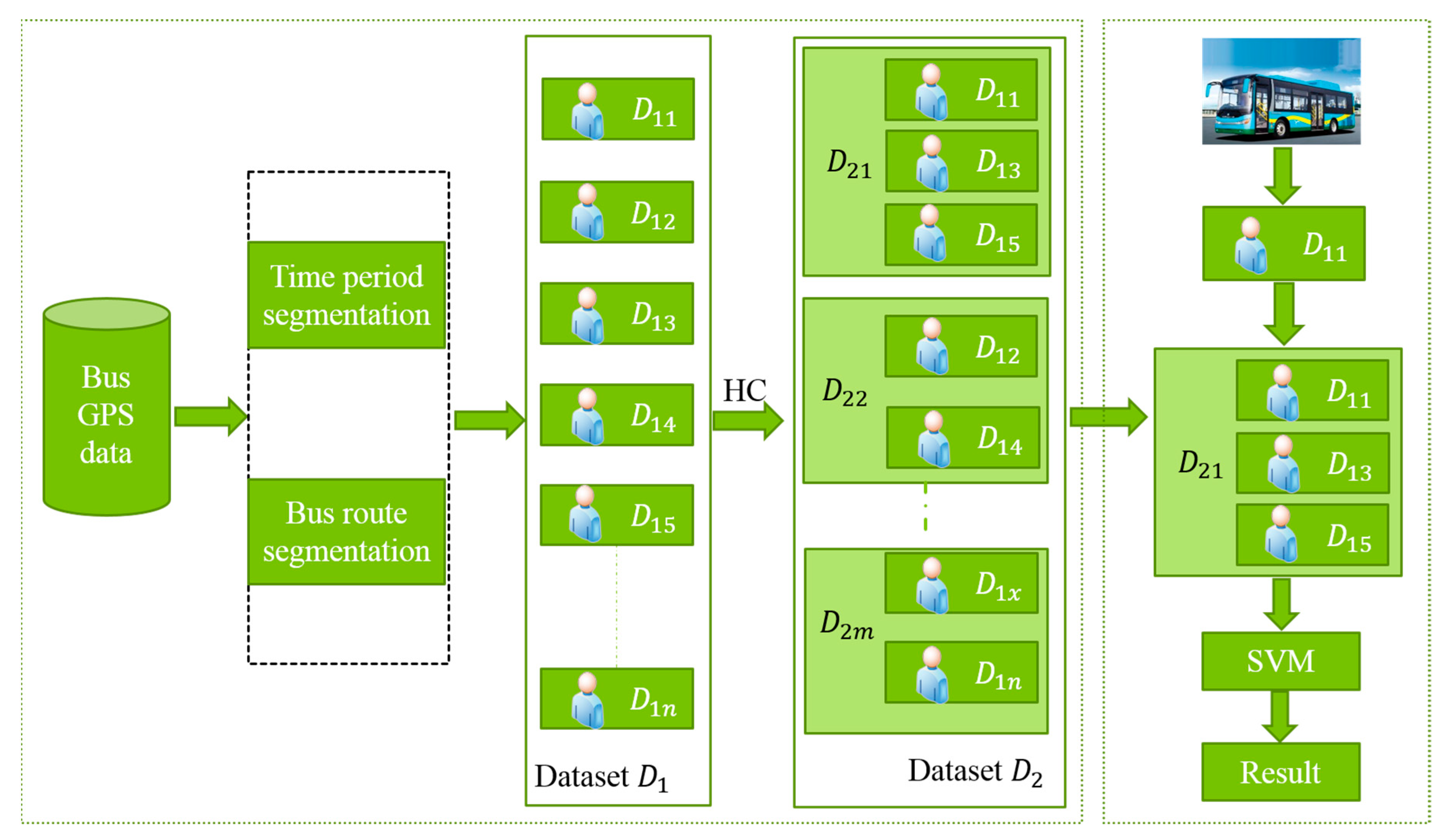
3.1. Prediction Framework
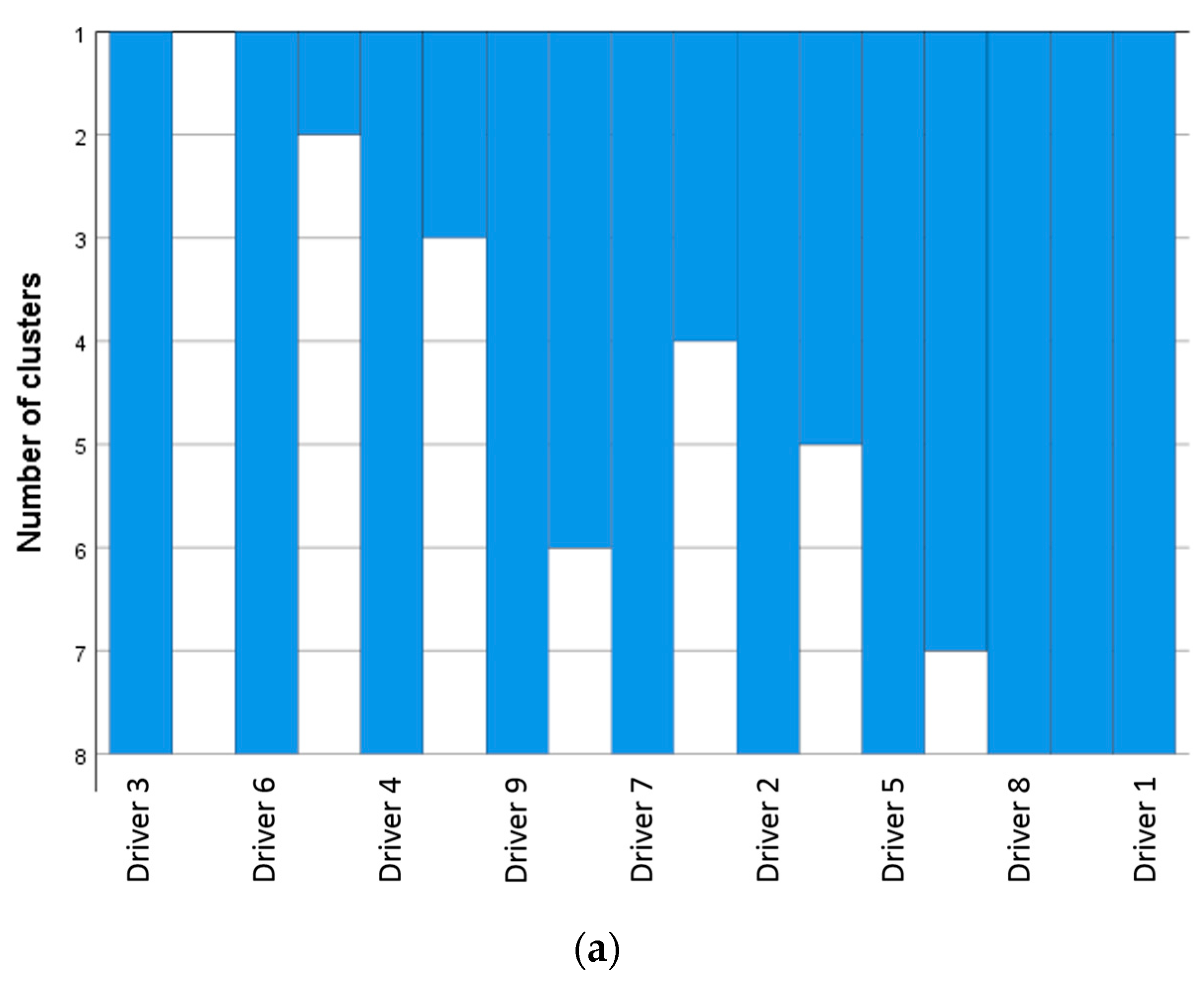
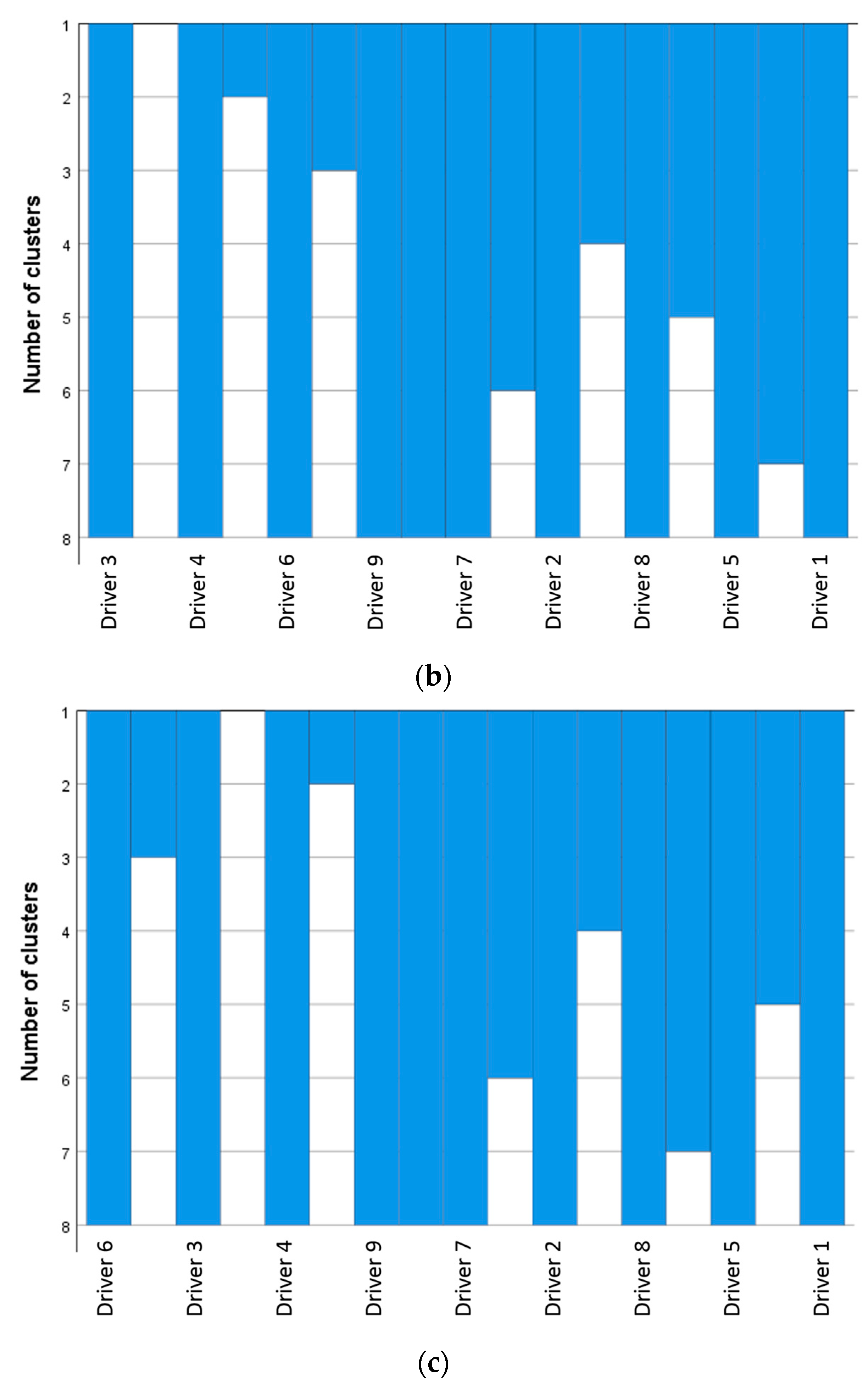
3.2. Driver Driving Style Classification Method
| Algorithm 1: HC—Basic Hierarchical Clustering Algorithm |
| Input: Sample set D = {}; Cluster distance metric function d; Number of clusters k. Output: Clusters C = {} Process: 1: for j = 1, 2, …, m do |
| 2: |
| 3: end for |
| 4: for i = 1, 2, …, m do 5: for j = i + 1, …, m do 6: M(i j) = d(); 7: M(j, i) = M() 8: end for 9: end for 10: Set the current number of clusters: q = m 11: while q > k do 12: Find the two closest clusters and ; 13: Merge and ; = ; 14: for do 15: Renumber cluster to 16: end for 17: Delete the row and column of the distance matrix M; 18: for j = 1, 2,…, q − 1 do 19: M() = d(); 20: 21: end for 22: q = q − 1 23: end while |
3.3. Bus Travel Time Prediction Method
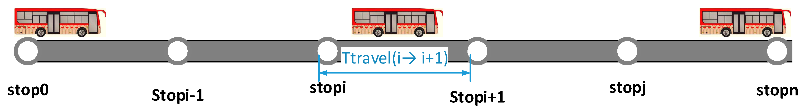
- is the predicted time for the bus to travel from stop i to stop i + 1, including the parking time at stop i, as shown in Figure 3;
- is the predicted arrival time of the bus at stop i;
- is the predicted arrival time of the bus at stop i + 1;
- (1)
- = day of the week. In general, traffic flow is different during the five working days of the week;
- (2)
- = number of road segments. The number of sections between two adjacent stops of the predicted bus line. Different road sections have different road condition characteristics;
- (3)
- = departure time of the bus. At different times of the day, the bus journey time is different. For example, during peak hours and off-peak hours, the travel time of buses varies greatly.
4. Case Study
4.1. Data Collection and Processing
4.2. Performance Measures
4.3. Driving Style Cluster of Bus Drivers
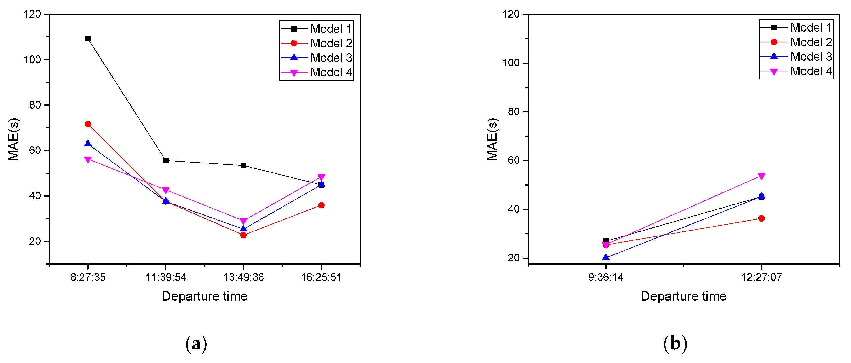
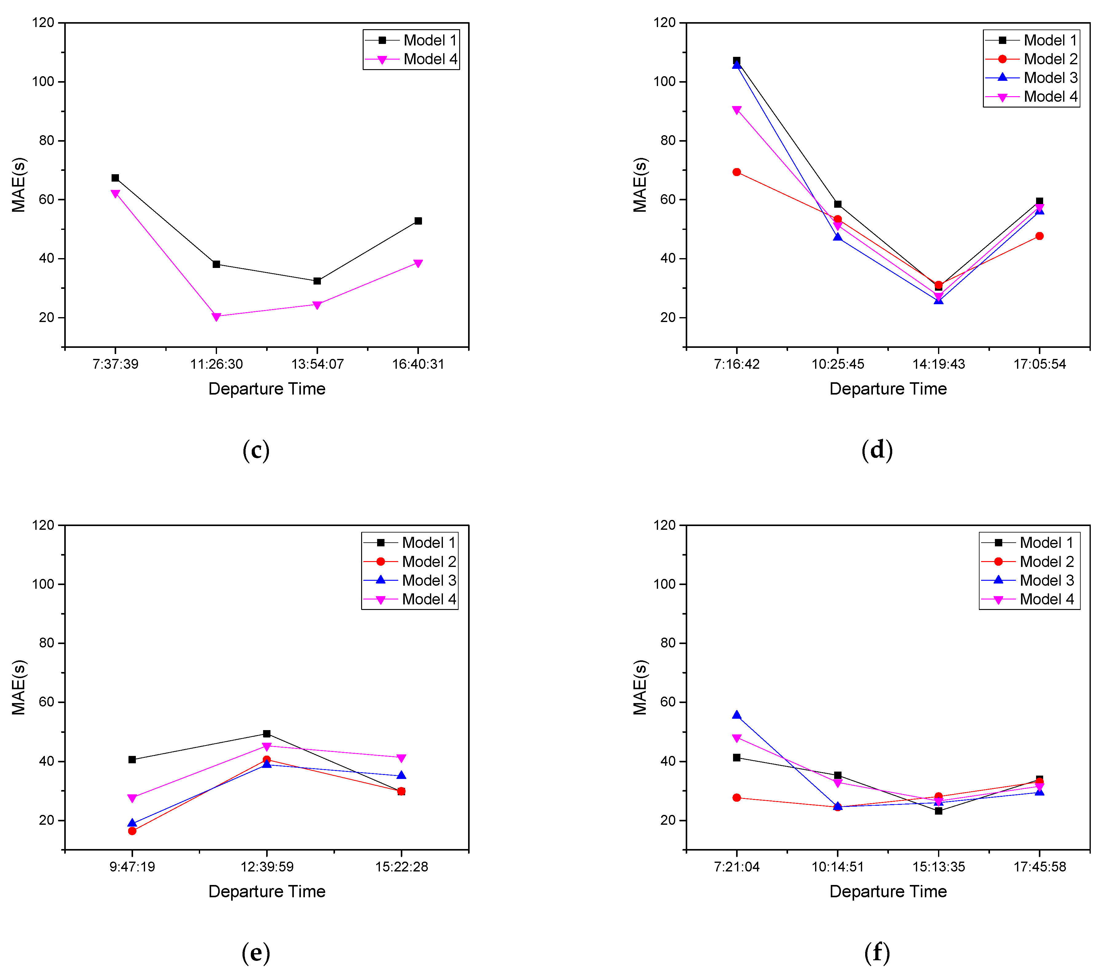
4.4. Results
4.5. Discussion
5. Conclusions
Author Contributions
Funding
Data Availability Statement
Conflicts of Interest
References
- Jeong, R.; Rilett, L.R. Bus arrival time prediction using artificial neural network model. In Proceedings of the 7th IEEE Intelligent Transportation System Conference, Washington, DC, USA, 3–6 September 2004. [Google Scholar] [CrossRef]
- Fan, W.; Gurmu, Z. Dynamic Travel Time Prediction Models for Buses Using Only GPS Data. Int. J. Transp. Sci. Technol. 2015, 4, 353–366. [Google Scholar] [CrossRef]
- Yu, B.; Wang, H.; Shan, W.; Yao, B. Prediction of bus travel time using random forests based on near neighbors. Comput. Aided Civ. Infrastruct. Eng. 2018, 33, 333–350. [Google Scholar] [CrossRef]
- Wei, M.; Liu, X. How wet is too wet? Modelling the influence of weather condition on urban transit ridership. Travel Behav. Soc. 2022, 27, 117–127. [Google Scholar] [CrossRef]
- O’Sullivan, A.; Pereira, F.C.; Zhao, J.; Koutsopoulos, H.N. Uncertainty in Bus Arrival Time Predictions: Treating Heteroscedasticity with a Metamodel Approach. IEEE Trans. Intell. Transp. Syst. 2016, 17, 3286–3296. [Google Scholar] [CrossRef]
- Yin, T.; Zhong, G.; Zhang, J.; He, S.L.; Ran, B. A prediction model of bus arrival time at stops with multi-routes. Transp. Res. Procedia 2017, 25, 4627–4640. [Google Scholar] [CrossRef]
- Ma, J.; Chan, J.; Ristanoski, G.; Rajasegarar, S.; Leckie, C. Bus travel time prediction with real-time traffic information. Transp. Res. Part C Emerg. Technol. 2019, 105, 536–549. [Google Scholar] [CrossRef]
- Daganzo, C.F. A headway-based approach to eliminate bus bunching: Systematic analysis and comparisons. Transp. Res. Part B Methodol. 2009, 43, 913–921. [Google Scholar] [CrossRef]
- Cats, O. Regularity-driven bus operation: Principles, implementation and business models. Transp. Policy 2014, 36, 223–230. [Google Scholar] [CrossRef]
- Yao, B.; Hu, P.; Lu, X.; Gao, J.; Zhang, M. Transit network design based on travel time reliability. Transp. Res. Part C Emerg. Technol. 2014, 43, 233–248. [Google Scholar] [CrossRef]
- Yu, H.; Chen, D.; Wu, Z.; Ma, X.; Wang, Y. Headway-based bus bunching prediction using transit smart card data. Transp. Res. Part C Emerg. Technol. 2016, 72, 45–59. [Google Scholar] [CrossRef]
- Martinez, C.M.; Heucke, M.; Wang, F.-Y.; Gao, B.; Cao, D. Driving Style Recognition for Intelligent Vehicle Control and Advanced Driver Assistance: A Survey. IEEE Trans. Intell. Transp. Syst. 2018, 19, 666–676. [Google Scholar] [CrossRef]
- Ahn, K.; Rakha, H.; Trani, A.; Van Aerde, M. Estimating vehicle fuel consumption and emissions based on instantaneous speed and acceleration levels. J. Transp. Eng. 2002, 128, 182–190. [Google Scholar] [CrossRef]
- Mudgal, A.; Hallmark, S.; Carriquiry, A.; Gkritza, K. Driving behavior at a roundabout: A hierarchical Bayesian regression analysis. Transp. Res. Part D Transp. Environ. 2014, 26, 20–26. [Google Scholar] [CrossRef]
- Johnson, D.A.; Trivedi, M.M. Driving style recognition using a smartphone as a sensor platform. In Proceedings of the 2011 14th International IEEE Conference on Intelligent Transportation Systems (ITSC), Washington, DC, USA, 5–7 October 2011; pp. 1609–1615. [Google Scholar] [CrossRef]
- Murphey, Y.L.; Milton, R.; Kiliaris, L. Driver’s style classification using jerk analysis. In Proceedings of the 2009 IEEE Workshop on Computational Intelligence in Vehicles and Vehicular Systems, Nashville, TN, USA, 30 March–2 April 2009; pp. 23–28. [Google Scholar] [CrossRef]
- Langari, R.; Won, J.-S. Intelligent energy management agent for a parallel hybrid vehicle—Part I: System architecture and design of the driving situation identification process. IEEE Trans. Veh. Technol. 2005, 54, 925–934. [Google Scholar] [CrossRef]
- Doshi, A.; Trivedi, M.M. Examining the impact of driving style on the predictability and responsiveness of the driver: Real-world and simulator analysis. In Proceedings of the 2010 IEEE Intelligent Vehicles Symposium, La Jolla, CA, USA, 21–24 June 2010; pp. 232–237. [Google Scholar] [CrossRef]
- Miyajima, C.; Nishiwaki, Y.; Ozawa, K.; Wakita, T.; Itou, K.; Takeda, K.; Itakura, F. Driver modeling based on driving behavior and its evaluation in driver identification. Proc. IEEE 2007, 95, 427–437. [Google Scholar] [CrossRef]
- Constantinescu, Z.; Marinoiu, C.; Vladoiu, M. Driving style analysis using data mining techniques. Int. J. Comput. Commun. Control 2010, 5, 654–663. [Google Scholar] [CrossRef]
- Vaitkus, V.; Lengvenis, P.; Zylius, G. Driving style classification using long-term accelerometer information. In Proceedings of the 2014 19th International Conference on Methods and Models in Automation and Robotics (MMAR), Miedzyzdroje, Poland, 2–5 September 2014; pp. 641–644. [Google Scholar] [CrossRef]
- Karginova, N.; Byttner, S.; Svensson, M. Data-Driven Methods for Classification of Driving Styles in Buses; SAE International: Warrendale, PA, USA, 2012. [Google Scholar] [CrossRef]
- Augustynowicz, A. Preliminary classification of driving style with objective rank method. Int. J. Automot. Technol. 2009, 10, 607–610. [Google Scholar] [CrossRef]
- Xu, L.; Hu, J.; Jiang, H.; Meng, W. Establishing style-oriented driver models by imitating human driving behaviors. IEEE Trans. Intell. Transp. Syst. 2015, 16, 2522–2530. [Google Scholar] [CrossRef]
- Zhu, L.; Yu, F.R.; Wang, Y.; Ning, B.; Tang, T. Big data analytics in intelligent transportation systems: A survey. IEEE Trans. Intell. Transp. Syst. 2019, 20, 383–398. [Google Scholar] [CrossRef]
- Patnaik, J.; Chien, S.; Bladikas, A. Estimation of bus arrival times using APC data. J. Publ. Transp. 2004, 7, 1–20. [Google Scholar] [CrossRef]
- Chien, S.I.-J.; Ding, Y.; Wei, C. Dynamic bus arrival time prediction with artificial neural networks. J. Transp. Eng. 2002, 128, 429–438. [Google Scholar] [CrossRef]
- Chen, M.; Liu, X.; Xia, J.; Chien, S.I. A dynamic bus-arrival time prediction model based on APC data. Comput.-Aided Civ. Infrastruct. Eng. 2004, 19, 364–376. [Google Scholar] [CrossRef]
- van Lint, J.W.C.; Hoogendoorn, S.P.; van Zuylen, H.J. Accurate freeway travel time prediction with state-space neural networks under missing data. Transp. Res. Part C Emerg. Technol. 2005, 13, 347–369. [Google Scholar] [CrossRef]
- Yu, B.; Lam, W.H.K.; Tam, M.L. Bus arrival time prediction at bus stop with multiple routes. Transp. Res. Part C Emerg. Technol. 2011, 19, 1157–1170. [Google Scholar] [CrossRef]
- Wu, C.-H.; Ho, J.-M.; Lee, D.T. Travel-time prediction with support vector regression. IEEE Trans. Intell. Transp. Syst. 2004, 5, 276–281. [Google Scholar] [CrossRef]
- Vanajakshi, L.; Rilett, L.R. Support vector machine technique for the short term prediction of travel time. In Proceedings of the 2007 IEEE Intelligent Vehicles Symposium, Istanbul, Turkey, 13–15 June 2007; pp. 600–605. [Google Scholar] [CrossRef]
- Yu, B.; Yang, Z.Z.; Yao, B.Z. Bus arrival time prediction using support vector machines. J. Intell. Trans. Syst. 2006, 10, 151–158. [Google Scholar] [CrossRef]
- Shalaby, A.; Farhan, A. Prediction models of bus arrival and departure times using AVL and APC data. J. Public Transp. 2004, 7, 41–61. [Google Scholar] [CrossRef]
- Vanajakshi, L.; Subramanian, S.C.; Sivanandan, R. Travel time prediction under heterogeneous traffic conditions using global positioning system data from buses. IET Intell. Transp. Syst. 2009, 3, 1–9. [Google Scholar] [CrossRef]
- Bai, C.; Peng, Z.-R.; Lu, Q.-C.; Sun, J. Dynamic Bus Travel Time Prediction Models on Road with Multiple Bus Routes. Comput. Intell. Neurosci. 2015, 2015, 432389. [Google Scholar] [CrossRef]
- Zhou, Z.H. Machine Learning, 1st ed.; Tsinghua University Press: Beijing, China, 2016; pp. 214–216. [Google Scholar]
- Yin, Z.; Zhang, B. Construction of Personalized Bus Travel Time Prediction Intervals Based on Hierarchical Clustering and the Bootstrap Method. Electronics 2023, 12, 1917. [Google Scholar] [CrossRef]
- Shalaby, A.; Farhan, A. Bus travel time prediction model for dynamic operations control and passenger information systems. In Proceedings of the 82nd Annual Meeting of the Transportation Research Board, Washington, DC, USA, 12–16 January 2003. [Google Scholar]
- He, P.; Jiang, G.; Lam, S.-K.; Sun, Y. Learning heterogeneous traffic patterns for travel time prediction of bus journeys. Inf. Sci. 2020, 512, 1394–1406. [Google Scholar] [CrossRef]
- Huang, Y.P.; Chen, C.; Su, Z.C.; Chen, T.S.; Sumalee, A.; Pan, T.L.; Zhong, R.X. Bus arrival time prediction and reliability analysis: An experimental comparison of functional data analysis and Bayesian support vector regression. Appl. Soft Comput. 2021, 111, 107663. [Google Scholar] [CrossRef]
- Kumar, B.A.; Vanajakshi, L.; Subramanian, S.C. Bus travel time prediction using a time-space discretization approach. Transp. Res. Part C Emerg. Technol. 2017, 79, 308–332. [Google Scholar] [CrossRef]
- Hua, X.; Wang, W.; Wang, Y.; Ren, M. Bus arrival time prediction using mixed multi-route arrival time data at previous stop. Transport 2017, 33, 543–554. [Google Scholar] [CrossRef]
- Ma, Z.; Koutsopoulos, H.N.; Ferreira, L.; Mesbah, M. Estimation of trip travel time distribution using a generalized Markov chain approach. Transp. Res. Part C Emerg. Technol. 2017, 74, 1–21. [Google Scholar] [CrossRef]
- Yuan, Y.; Shao, C.; Cao, Z.; He, Z.; Zhu, C.; Wang, Y.; Jang, V. Bus Dynamic Travel Time Prediction: Using a Deep Feature Extraction Framework Based on RNN and DNN. Electronics 2020, 9, 1876. [Google Scholar] [CrossRef]
- Bie, Y.; Wang, D.; Qi, H. Prediction Model of Bus Arrival Time at Signalized Intersection Using GPS Data. J. Transp. Eng. 2012, 138, 12–20. [Google Scholar] [CrossRef]
- Chow, A.H.F.; Li, S.; Zhong, R. Multi-objective optimal control formulations for bus service reliability with traffic signals. Transp. Res. Part B Methodol. 2017, 103, 248–268. [Google Scholar] [CrossRef]


| Variable | Description |
|---|---|
| O_LINENAME | the line name |
| O_TERMINALNO | the serial number of the vehicle-mounted device |
| O_DATE | the date of data generated |
| O_TIME | the time of data generated |
| O_LONGITUDE | Longitude |
| O_LATITUDE | Latitude |
| O_SPEED | instantaneous speed |
| O_UP | running direction |
| O_NEXTSTATIONNO | the serial number of the next stop |
| Model | Number of Clusters | 7:00–9:00 | 9:00–16:00 | 16:00–19:00 |
|---|---|---|---|---|
| Model 1 | 9 | 902334 | 902334 | 902334 |
| Model 2 | 5 | 902334, 902335, 902349, 902355 | 902334, 902349, 902355 | 902334, 902349, 902359 |
| Model 3 | 4 | 902334, 902335, 902349, 902353, 902355, 902359 | 902334, 902335, 902349, 902353, 902355, 902359 | 902334, 902335, 902349, 902353, 902355, 902359 |
| Model 4 | 1 | All data | All data | All data |
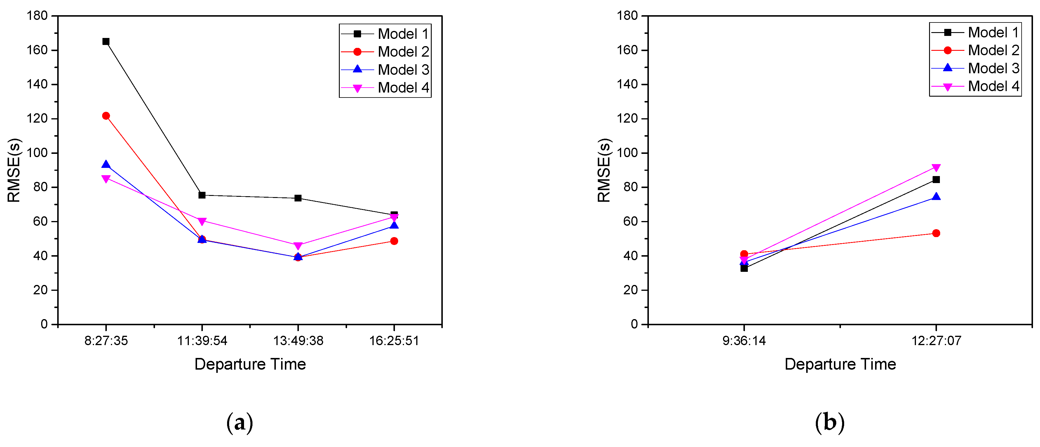
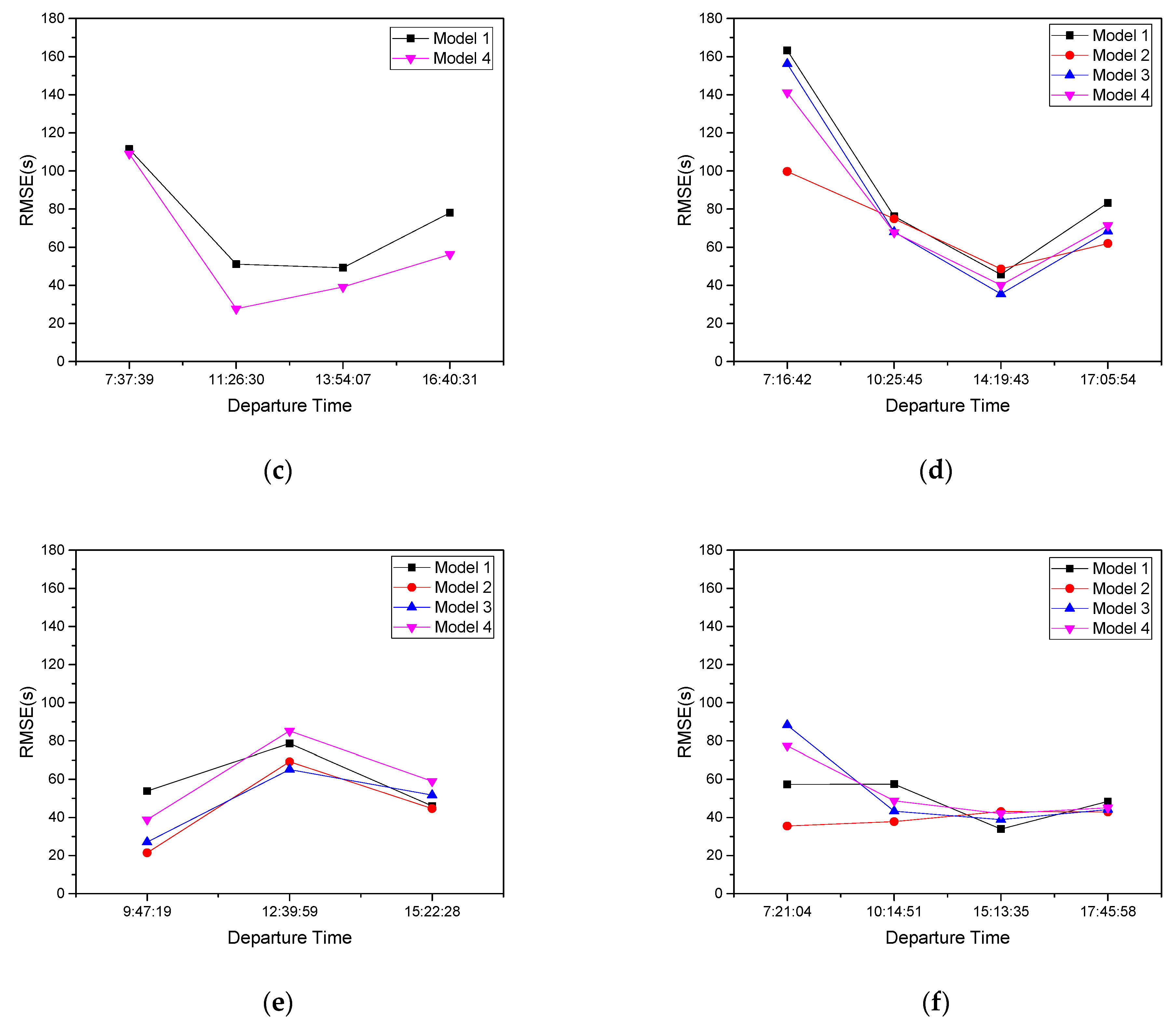
| Time Period | 902334 | 902335 | 902351 | 902353 | 902355 | 902359 |
|---|---|---|---|---|---|---|
| 7–9 | 8:27:35 | 7:37:39 | 7:16:42 | 7:21:04 | ||
| 9–12 | 11:39:54 | 9:36:14 | 11:26:30 | 10:25:45 | 9:47:19 | 10:14:51 |
| 12–16 | 13:49:38 | 12:27:07 | 13:54:07 | 14:19:43 | 12:39:59 15:22:28 | 15:13:35 |
| 16–19 | 16:25:51 | 16:40:31 | 17:05:54 | 17:45:58 |
| Driver | Model 1 | Model 2 | Model 3 | Model 4 |
|---|---|---|---|---|
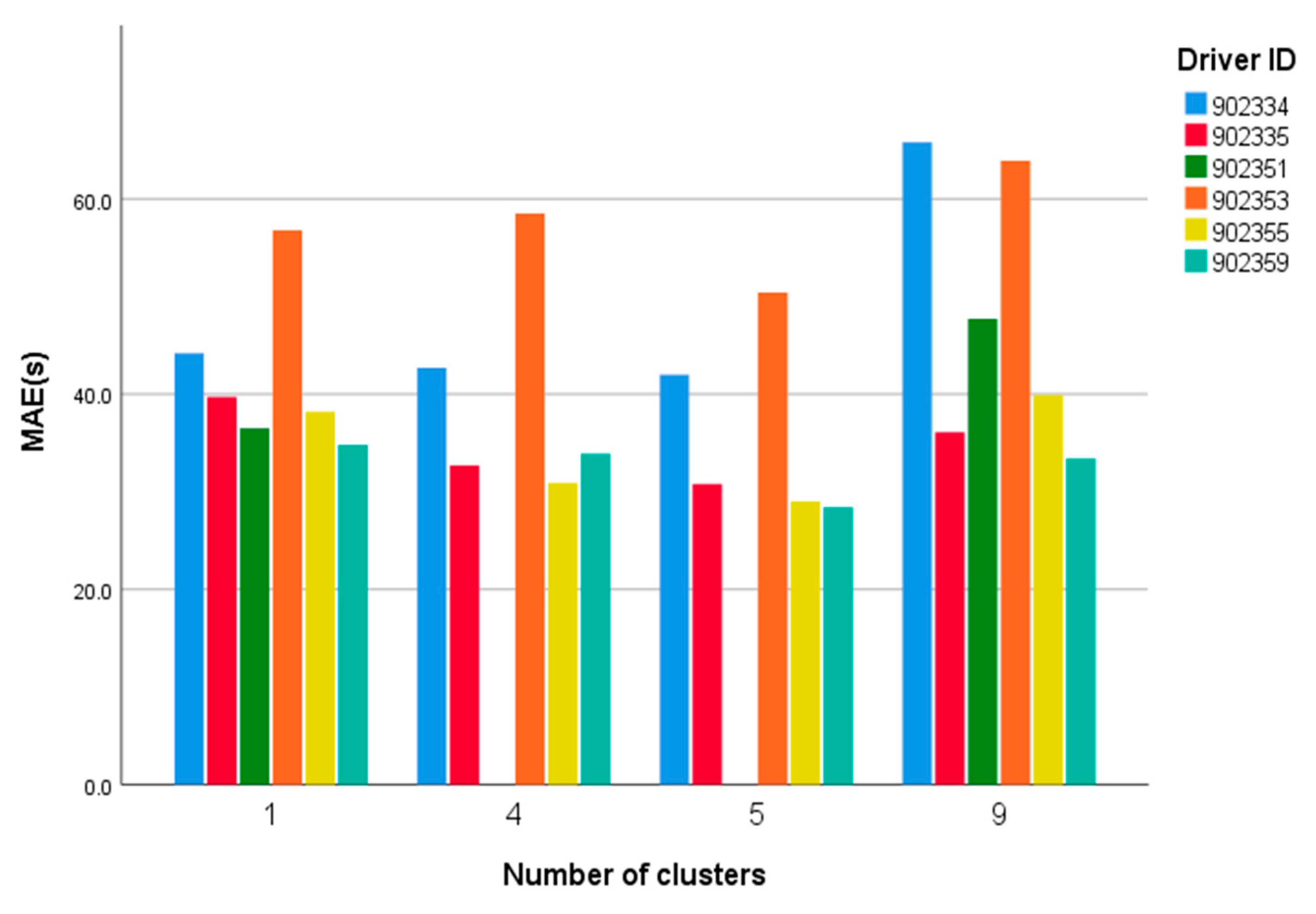
| 902334 | 65.8 | 42.0 | 42.7 | 44.2 |
| 902335 | 36.1 | 30.8 | 32.7 | 39.7 |
| 902351 | 47.7 | 36.5 | ||
| 902353 | 63.9 | 50.4 | 58.5 | 56.8 |
| 902355 | 39.9 | 29.0 | 30.9 | 38.2 |
| 902359 | 33.4 | 28.4 | 33.9 | 34.8 |
| g-MAE | 47.8 | 36.1 | 39.7 | 41.7 |
| Driver | Model 1 | Model 2 | Model 3 | Model 4 |
|---|---|---|---|---|
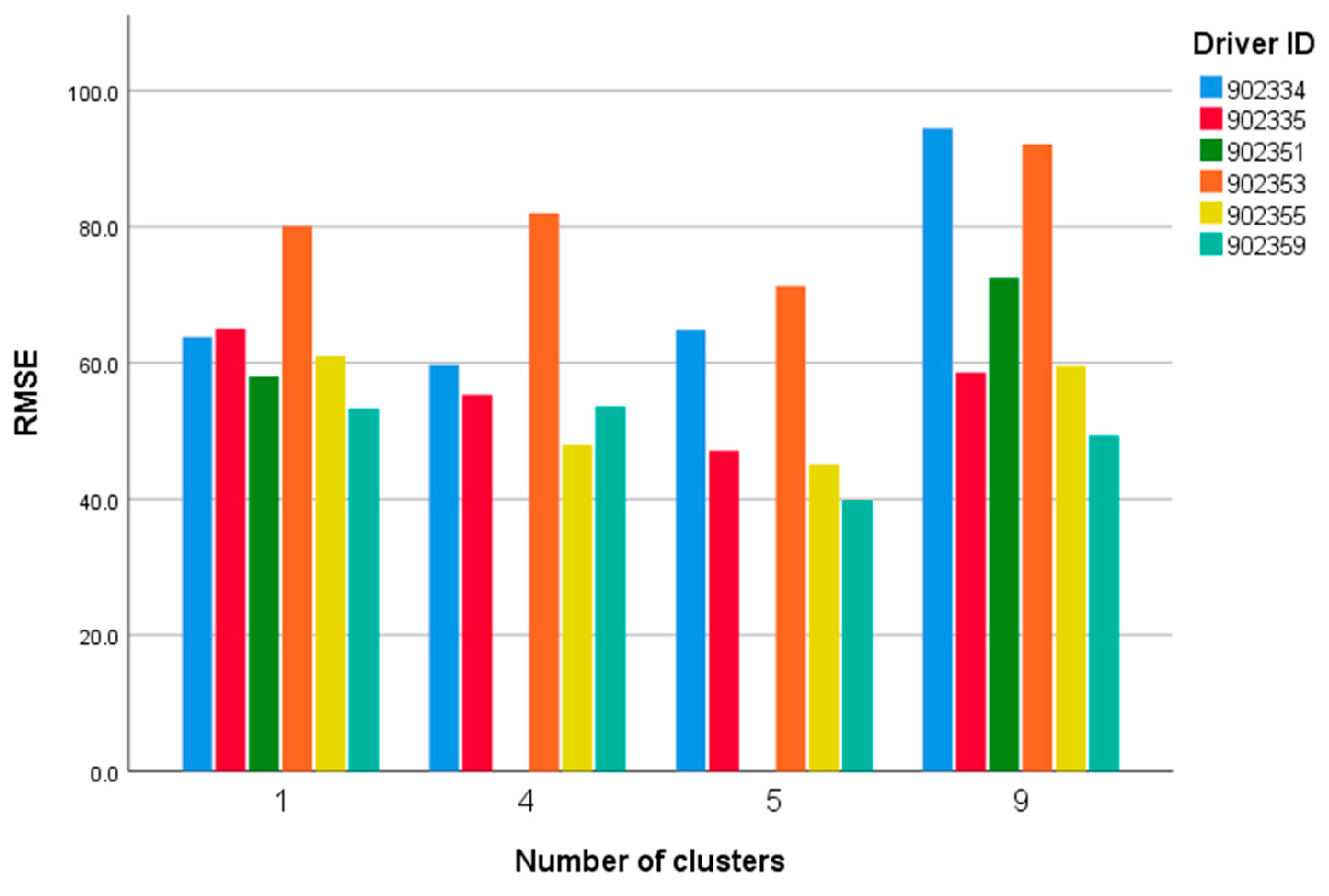
| 902334 | 94.5 | 64.8 | 59.7 | 63.8 |
| 902335 | 58.6 | 47.1 | 55.3 | 65.0 |
| 902351 | 72.5 | 58.0 | ||
| 902353 | 92.1 | 71.3 | 82.0 | 80.1 |
| 902355 | 59.5 | 45.1 | 48.0 | 61.0 |
| 902359 | 49.3 | 39.8 | 53.6 | 53.3 |
| g-RMSE | 71.1 | 53.6 | 59.7 | 63.5 |
Disclaimer/Publisher’s Note: The statements, opinions and data contained in all publications are solely those of the individual author(s) and contributor(s) and not of MDPI and/or the editor(s). MDPI and/or the editor(s) disclaim responsibility for any injury to people or property resulting from any ideas, methods, instructions or products referred to in the content. |
© 2023 by the authors. Licensee MDPI, Basel, Switzerland. This article is an open access article distributed under the terms and conditions of the Creative Commons Attribution (CC BY) license (https://creativecommons.org/licenses/by/4.0/).
Share and Cite
Yin, Z.; Zhang, B. Bus Travel Time Prediction Based on the Similarity in Drivers’ Driving Styles. Future Internet 2023, 15, 222. https://doi.org/10.3390/fi15070222
Yin Z, Zhang B. Bus Travel Time Prediction Based on the Similarity in Drivers’ Driving Styles. Future Internet. 2023; 15(7):222. https://doi.org/10.3390/fi15070222
Chicago/Turabian StyleYin, Zhenzhong, and Bin Zhang. 2023. "Bus Travel Time Prediction Based on the Similarity in Drivers’ Driving Styles" Future Internet 15, no. 7: 222. https://doi.org/10.3390/fi15070222
APA StyleYin, Z., & Zhang, B. (2023). Bus Travel Time Prediction Based on the Similarity in Drivers’ Driving Styles. Future Internet, 15(7), 222. https://doi.org/10.3390/fi15070222