Article

A Deep Learning Approach to Detect Failures in Bridges Based on the Coherence of Signals

Mechanical Department, Politecnico di Milano, Via G. La Masa, 1, 20156 Milan, Italy
*
Author to whom correspondence should be addressed.
Future Internet 2023, 15(4), 119; https://doi.org/10.3390/fi15040119
Submission received: 1 March 2023 / Revised: 21 March 2023 / Accepted: 23 March 2023 / Published: 25 March 2023
(This article belongs to the Special Issue Artificial Intelligence for Smart Cities)

Abstract

:
Structural health monitoring of civil infrastructure, such as bridges and buildings, has become a trending topic in the last few years. The key factor is the technological push given by new technologies that permit the acquisition, storage, processing and visualisation of data in real time, thus assessing a structure’s health condition. However, data related to anomaly conditions are difficult to retrieve, and, by the time those conditions are met, in general, it is too late. For this reason, the problem becomes unsupervised, since no labelled data are available, and anomaly detection algorithms are usually adopted in this context. This research proposes a novel algorithm that transforms the intrinsically unsupervised problem into a supervised one for condition monitoring purposes. Considering a bridge equipped with N sensors, which measure static structural quantities (rotations of the piers) and environmental parameters, exploiting the relationships between different physical variables and determining how these relationships change over time can indicate the bridge’s health status. In particular, this algorithm involves the training of N models, each of them able to estimate the quantity measured via a sensor by using the others’ N 1 measurements. Hence, the system can be represented by the ensemble of the N models. In this way, for each sensor, it is possible to compare the real measurement with the predicted one and evaluate the residual between the two; this difference can be addressed as a symptom of changes in the structure with respect to the condition regarded as nominal. This approach is applied to a real test case, i.e., Candia Bridge in Italy, and it is compared with a state-of-the-art anomaly detector (namely an autoencoder) in order to validate its robustness.

1. Introduction

To use a metaphor, infrastructural networks can be described as the veins and arteries of a country. Indeed, they allow for the flux of people and goods, which is essential for the flourishing of culture and economics. Among the components of traffic routes, bridges are the most impactful on a system’s resilience. Additionally, bridges are potentially subject to a very large spectrum of degradation processes linked to their constructive materials, structural characteristics and exposure to external agents [1,2,3]. This is why an efficient approach to the management and maintenance of these structures has always been considered of paramount importance, with the United States leading the way since the 1970s. The latter has become a hot topic in the last decade, made even more evident by serious facts and collapses happening worldwide with worrying frequency [4,5]. Many factors contribute to this process: in particular, the scientific literature on bridge safety affirms that ageing and damage caused by natural disasters are the most relevant threats to bridges’ integrity, with 7 out of 10 structural failures due to a combination of such factors [6,7]. To make things worse, data from the World Meteorological Organization report a concerning five-time increase in the occurrence of natural disasters over the past 50 years, mainly driven by climate change and more extreme weather conditions [8].
According to most countries’ policies, after such exceptional events affect a bridge, its structural safety should be assessed through extraordinary visual inspections, which oversee the deployment of testing equipment to check the status of the superstructure, substructure and underwater elements [9]. However, not only is this practice extremely expensive and time-consuming, but also, its results are questionable and surely not able to capture any phenomena of drift of the structural behaviour of the bridge, which are quantitative and evolve slowly over time [10,11]. Instead, the continuous monitoring of the bridge through sensors is much more informative. To make a comparison of the two techniques, continuous monitoring might be considered, for example, in the form of a video, while a visual inspection is more similar to a picture. On the other hand, a significant analysis effort is required to extract such valuable information from the huge amount of data produced daily by a monitoring system.
In this regard, machine learning represents a precious resource. The design and implementation of efficient algorithms based on artificial intelligence allow for analysing data from heterogeneous sensors simultaneously, making it possible to capture the complexity of a bridge’s structural behaviour. This approach can lead to more autonomous, accurate and robust processing of the monitoring data [12]. In recent years, researchers in the structural health monitoring (SHM) community have been exploring the potential applications of deep learning-based approaches for detecting structural damage and assessing the overall condition of structures. By leveraging the power of deep learning, these approaches have the potential to improve the reliability and efficiency of SHM systems, thereby enhancing the safety and performance of structures.
Jian et al. [13] demonstrated the effectiveness of a one-dimensional convolutional neural network (CNN) for anomaly identification with vibration signals in bridges. Bao et al. [14] proposed a novel data anomaly detection method that uses computer vision and deep learning techniques. This approach involves converting the original time series measurement values into image vectors, which are then input to a deep neural network to detect various anomalies. In their study, Mousavi and Gandomi [15] employed an approach to detect damages in structures by training an RNN using the natural frequency and corresponding Johansen cointegration residuals, by removing seasonal patterns from the data with variational mode decomposition algorithm. Ni et al. [16] proposed a novel deep learning-enabled data compression and reconstruction framework based on two different networks: a CNN that extracts features directly from the input signals to detect anomalous data and a data compression and reconstruction method based on an autoencoder, which can recover the data. Mao et al. [17] adopted generative adversarial networks and autoencoders to recognise anomaly conditions.
This paper contributes to the literature by proposing a deep-learning-based approach. The proposed algorithm relies on the analysis of the signal’s coherence: given an acquisition system made of N sensors, the idea is to train N models iteratively, estimating the readings of one sensor by using all of the other nodes of the acquisition network. The result is an anomaly detection system that can localise and quantify anomalous behaviour. Moreover, being that the model is totally data-driven, it requires no previous knowledge of the structure, can be applied to sensors of different natures and is characterised by a fast deployment on existing time series.
The validation of this approach has been carried out by applying it to a masonry arch bridge in Italy, which allowed for the detection and localisation of a flood’s effects. The bridge, which flooded in October 2020, has been endowed with a monitoring system to collect data since December 2020 [18]. The proposed algorithm is compared with another one, which analogously performs data fusion on signals from tiltmeters installed on the structure, with the aim of tracking the bridge’s structural behaviour.
The proposed methodology successfully identified the transient between the flood and the stabilisation on a new equilibrium position. This is a really valuable result because it helps ensure the bridge’s structural safety after such an extreme event, thus supporting the maintenance of the infrastructural network by providing quantitative and reliable information.
The paper is organised as follows: in Section 2, the experimental setup and a description of the available dataset are outlined; in Section 3, a novel methodology is introduced and compared with a state-of-the-art algorithm; in Section 4, a discussion on data preprocessing and algorithm architecture is described; in Section 5, the methodology is applied to a real test case to prove its robustness; and, finally, conclusions are drawn.

2. Experimental Set Up

The monitoring system installed on this bridge (represented in Figure 1) acquires data continuously. Candia Bridge is a multi-span masonry arch bridge that is monitored mainly by tiltmeters, which are used to assess the static position of the bridge. In particular, MEMS tiltmeters (hereafter denoted by Txx) are placed on the arches skewback and are in charge of recording the transversal rotation (positive if upriver) of the piers. In fact, as an example, a possible flooding scenario can apply a scouring action on the foundation by determining (in the long period) potentially irreversible rotations. Moreover, a weather station is placed in the middle of the bridge to record different environmental factors: the pressure, internal temperature of the station, external air temperature, internal humidity, external humidity, wind speed, speed direction and rain rate. Tiltmeters 2 and 14 are equipped with an internal temperature sensor that is stored during the acquisition.
To detect extraordinary events, the bridge is equipped with hydraulic and visual sensors too:
  • Hydrometer: measures the river level identifying possible flooding that can be dangerous for the bridge’s structure.
  • Echo sounder: measures the level of the river bed and can provide information about possible movements of the piers within its proximity.
  • Cameras: identify possible detritus stacks at the base of the piers by documenting and characterising the annual process of plant transportation.
A strengthening intervention was made on the river bed in 2003; it is noticed that the piers located within the working site are more subjected to the scouring action. On these piers, two tiltmeters are installed; to better describe this phenomenon, they are placed on the arch skewback converging on the pier.

Dataset Acquisition

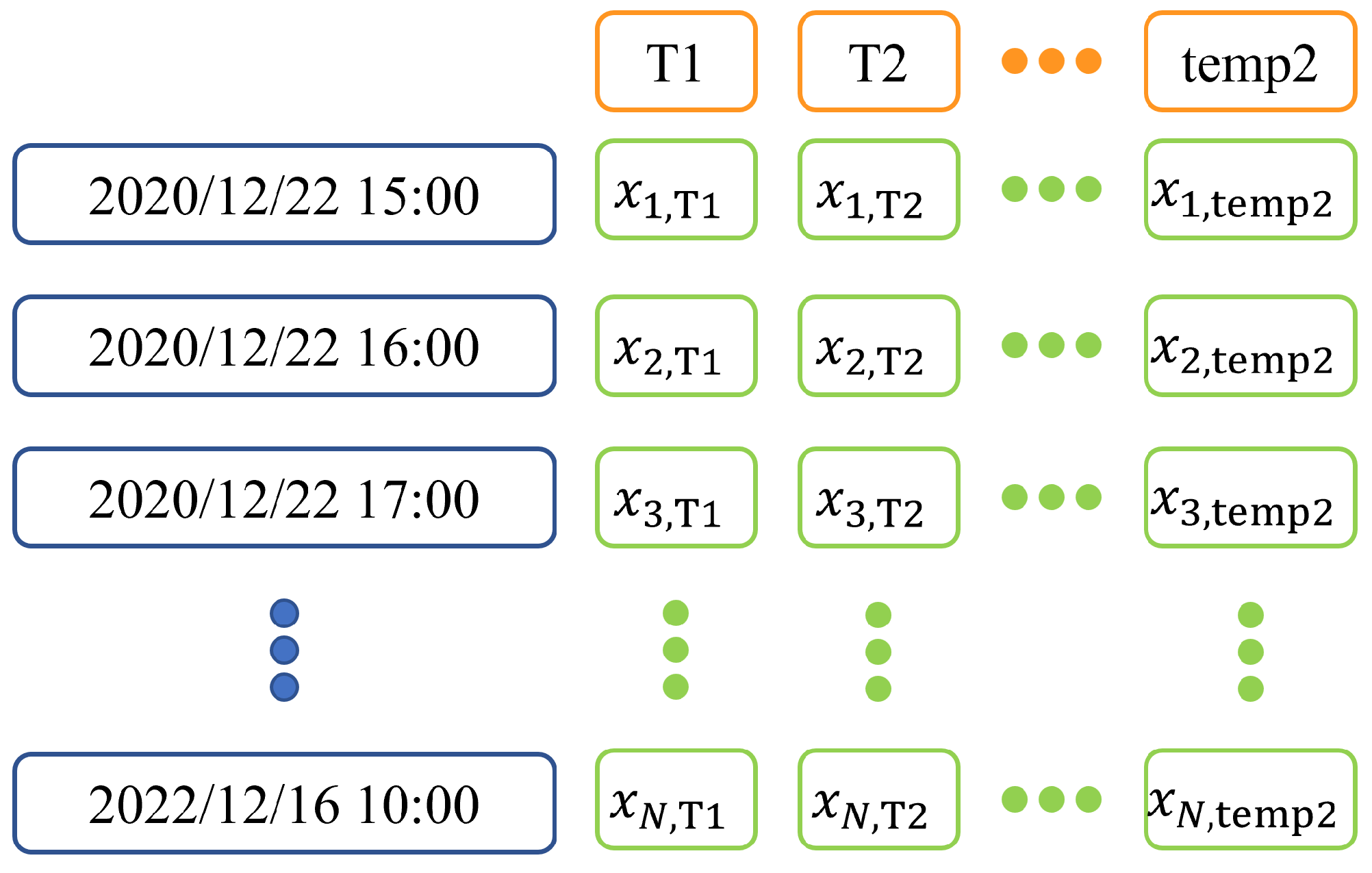
The dataset available for this research consists of the measurements acquired from all of the sensors summarised in Table 1. The temperatures corresponding to channels 23 and 24 are extracted from tiltmeters 2 and 14. The temperatures in channels 26 and 27 (hereafter called Temp1 and Temp2) refer instead to the internal and external temperatures measured by the weather station. All of the signals have been acquired with a sampling frequency of 1 Hz. To make the models more robust against random noise and reduce the storage space, the data have been averaged on an hourly basis, so that every channel counts one value per hour. In Figure 2, the arrangement of the data after preprocessing is reported. The dataset consists now of a matrix, where each row corresponds to a timestamp and each column corresponds to a sensor. A new row is generated every hour.
The acquisition period spans from December 2020 to December 2022. It is important to underline that, in October 2020, the city of Candia Lomellina was hit by a flood that caused damage in this area, and, in particular, another bridge collapsed on this occasion. In the next section, it will be demonstrated how Candia Bridge was affected by this phenomenon by moving away from its equilibrium position and finding a new, stable one in the summer of 2021.

3. Multi-Input Machine Learning Modelling

Although simple models such as linear regressions are easy to interpret and give a sufficiently accurate description of bridge physics, they have some intrinsic limits. For instance, the number of inputs that can be introduced while keeping a representation of the laws understandable for humans is usually no more than two, so that the model can be represented in a 3D space. In addition, linear models are characterised by a limited number of parameters, having then an inadequate capability to represent the behaviour of complex systems, particularly when they are evolving in time. It can, consequently, be beneficial to model the system by contemplating more inputs and models characterised by more parameters. Fully data-driven modelling of the system is then suitable for this purpose. The problem of structural health monitoring with an unsupervised dataset is commonly regarded as novelty detection or anomaly detection [19]. The logic is to use the training data to establish the nominal condition of the structure. The monitoring system must be then able to identify a modification in the system. Before fitting any model into the dataset, a baseline must be defined, that is, the portion of the dataset corresponding to periods where the structure is regarded as healthy. In practice, given a time series matrix X R n × m , made of n measurements for m time “snapshots”:
X = x 1 , x 2 , , x m
and defining the training set finally consists in selecting the proper k < m so that:
X train = x 1 , x 2 , , x k

3.1. Iterative Models

The dataset collected from a structure is unsupervised most of the time, namely a dataset with no specific labels (numerical or categorical) associated with the dataset objects. Most of the unsupervised approaches rely on the detection of the dataset modifications. However, in this way, the monitoring system is only able to identify whether something has changed, without actually localising where the modification took place [20]. A possible approach to overcome these limitations could be to turn the unsupervised problem into a supervised one. For example, some health monitoring algorithms are based on the use of environmental variables (such as temperatures) as the input of a regressor, which must estimate the features extracted from the sensors. This allows the normalisation of the signals with respect to the environmental effects, before applying an anomaly detection algorithm that is usually based on statistics [21,22]. If the physical variables measured are static, which means they measure low-frequency variations only, this procedure can be applied directly to the sensors’ readings, without any particular feature extraction.
Among the possible machine learning methods for regression, neural networks are among the most flexible ones. The layers of neural networks can be selected and adjusted to take in input and output tensors of any size. It is then possible to divide the sensors mounted on the structure into groups according to the type of physical quantity that they measure (tiltmeter, strain gauges, thermometers, etc.) or their location (first span of the bridge, second span, and so on) and then train a neural network so that it can use one group from the input to estimate the values of the sensors of another group. Then, the residuals e i j can be computed as:
e i j = y i j y ^ i j
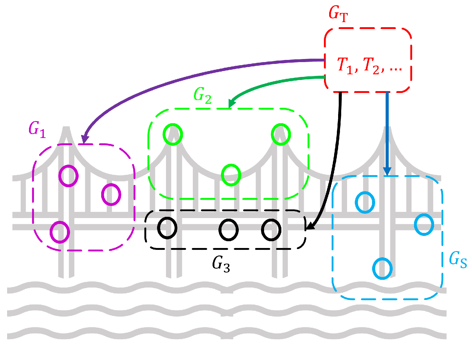
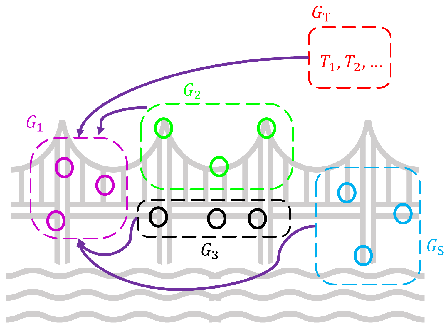
where y i j and y ^ i j refer to the measured value and the value estimated by the neural network, respectively, while the subscript i refers to the i t h sensor considered and j to the j t h timestamp. The residuals can then be used as an indicator of the structure’s health condition. In this way, the normalisation of the signals with respect to the environmental effect can just be seen as a particular case of this procedure, where the inputs of the neural network are the temperatures and the output of a group (or multiple groups) of sensors, as shown in Figure 3. By following this procedure, the residuals obtained represent all the disturbances that cannot be attributed to temperatures. However, one might also focus on one single group and establish the effect of all of the other groups of sensors (Figure 4). The physical meaning of residuals is now different compared to the case where only the temperatures are used as the input. Now the model takes into account the readings of sensors of different natures. Therefore, the residuals are proportional to the level of coherence of one group of sensors with respect to the others. By iterating the process for all groups of sensors, given G groups, every iteration consists of the training of G models, so that each of them estimates the value of one group of sensors taking into account the other G 1 .
The logical extension of this procedure is to consider only the groups made of one single sensor (leave-one-out strategy). If N sensors are mounted on the structure, this strategy involves the training of N neural networks, so that at every iteration the neural network estimates the value of one single sensor by taking the other N 1 ones as the input. Eventually, a comprehensive model made of N neural networks is associated with the structure. For simplicity, we call this “comprehensive” model an iterative model. It is worth mentioning that the iterative model can be made of other machine learning regressive models rather than neural networks, since the output is, in this case, a single continuous variable. [23,24]. By considering the set of measurements Y j = y 1 j , , y n j available at the j t h timestamp, the iterative model can synthetically be represented by the system:
y ^ i j = f ^ i ( X i j ) for i = 1 , , n
where X i j = Y j { y i j } represents the set of values measured by all the sensors except the i t h one, whereas f ^ i is the regressor able to estimate the value of the i t h sensor from X i j . Finally, the residuals can be computed with Equation (3). In this context, the residuals represent how distant the value measured by a sensor is from the expected one, and, therefore, the equation quantifies coherence among all sensors’ readings. This approach reaches level 2 in the SHM hierarchical structure, namely the localisation of damage, as well as its assessment, even if only to a limited degree. In this regard, it is necessary to remark on an important aspect: the application of an iterative model to a new observation Y new will produce a vector of residuals: E new = e 1 , new , , e n , new , which must show low values in the case of a healthy structure. In addition, in the case of damage caused at the i t h sensor, the residual vector E new is expected to feature a “spike” in the i t h residual e i , new . However, since y i , new is the input for the other sensors, an increase in the residuals will be seen in all of the other elements of the vector E new . Therefore, the damage identification capability is maintained as long as the residual in the i t h position of E new grows more than the others. However, since the method is fully data-driven, it is hard to define when and how this might happen. During the monitoring phase, some statistical considerations can be carried out on the vector of residuals E to define the confidence level for raising warnings.
It is worth mentioning that this algorithm has been tested on two other bridges that were monitored for about one and a half years. Iterative models were trained over a one-year time span and tested on the remaining period. In both structures, no anomaly conditions were recorded since the obtained residuals for all of the sensors maintained low values in time, comparable to the training loss. However, in this paper, the results related to these two bridges are not included because the authors want to focus on a test case in which a real anomaly condition has been met and correctly identified. In fact, a flood is an exceptional event that has hardly been encountered in previous research works related to bridge monitoring.
Due to the limited period of monitoring, it is not possible to be sure that the algorithm is robust to long-term changes. However, due to the fact that it evaluates the coherence of the different signals and, indirectly, the measurement of a single variable, it is realistic to suppose that it will be robust to long-term changes. If the algorithm finds a change in the system, it can be a preliminary warning that an inspection or, more generally, an evaluation of the bridge is required. If after the inspection, the bridge is considered healthy, it is possible to retrain the model and, therefore, to define a new nominal condition.

3.2. Autoencoder Model

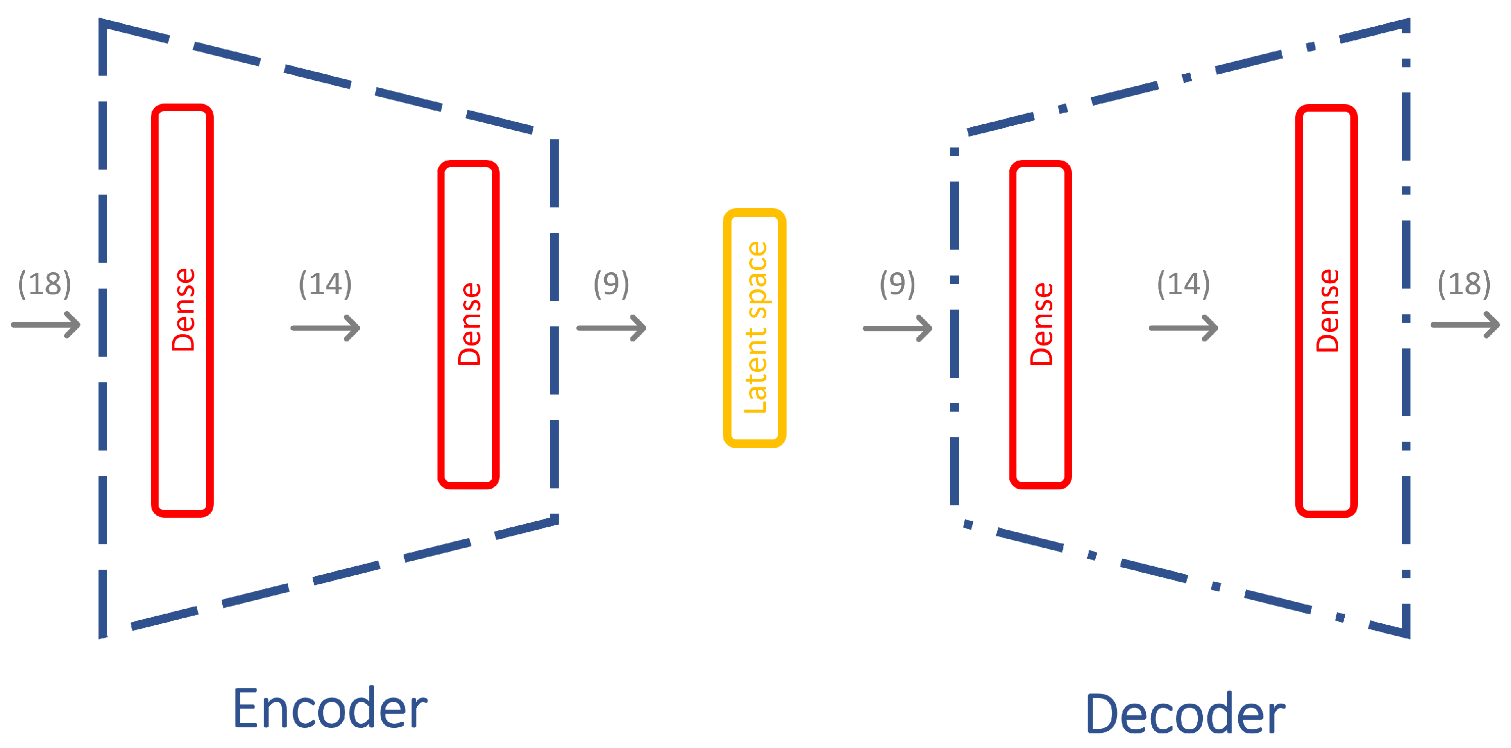
To evaluate the performance of iterative models, a comparison with the state-of-the-art autoencoder (AU) algorithm is carried out. The AU has been regarded as an anomaly detector algorithm [17,25,26], which can be applied in applications where it is necessary to establish whether a system is moving away from the nominal condition. This algorithm (represented in Figure 5) is a particular type of neural network that performs two main operations:
  • Encoder function: it applies different transformations to the input data ( X ) by means of successive layers, which generates a compressed representation of the input ( H ) in a new feature space usually called latent space. The mathematical expression is: H = f ( X ) .
  • Decoder function: starting from the latent space, it applies different transformations to determine a reconstruction ( R ) of the input. The mathematical expression is: R = g ( H ) .
To evaluate the performance in reconstructing the input, the residual between the input and output is evaluated:
E AU = R X
where R and X are vectors with dimensions N × 1 (number of measurements). So, e AU is a vector with the same dimension, whose elements represent the reconstruction error for all measurements. If the AU is trained with nominal data, it learns to minimise the reconstruction error when nominal data are processed and to raise it when anomalous data are encountered.

4. Data Preprocessing and Models Architecture

As already explained in Section 2, the data are averaged on an hourly basis, so that every channel counts one value per hour. A preliminary statistical analysis of the data led to not considering some measurements when constructing the model; in particular, the different models consider the 15 tiltmeters, the hydrometer level and the two temperatures Temp1 and Temp2. The other variables are not taken into account since they are not related to the bridge’s behaviour.
To bring the data in the format required for their processing with neural networks, some manipulations are performed according to the method described in [27]. Firstly, the data are arranged in a matrix, whose dimensions are N samples × 18 , with 18 being the number of measurements used by the model. Secondly, each column of the matrix for the training set is normalised by adopting a standardisation technique [28]:
z i j = x i j μ j σ j for j = 1 , , 17 and i = 1 , , N samples
where μ j and σ j , respectively, represent the mean value and the standard deviation for the measure of the j t h sensor in the training set. In this way, the distribution of samples for each variable will be centred on zero with a standard deviation of 1.
For the iterative models, the dimensions of the input–output tensors, respectively, become N samples × 17 and N samples × 1 . The architecture of the network (represented in Figure 6) is made of two dense layers with the ReLU activation function, a dropout layer to avoid overfitting [29] and a final dense output with a linear activation function.
While for the AU model, the input and output of the network are the same, including all the measurements available, i.e., a matrix with the dimensions N samples × 18 . The architecture, in this case, is represented in Figure 7.
For the case study of Candia Bridge, the model is trained with data from December 2021 to December 2022, during which the bridge is considered in a new, stable equilibrium position. The testing phase is then performed on data from December 2020 to November 2021 to verify the hypothesis that the bridge was in a “transitory” phase due to the flood event. The objective is first to assess if the bridge is in stable condition at the end and to find the moment at which it arrived to this condition; in this way, it is possible to assess the bridge’s safety after an extraordinary event.

5. Results

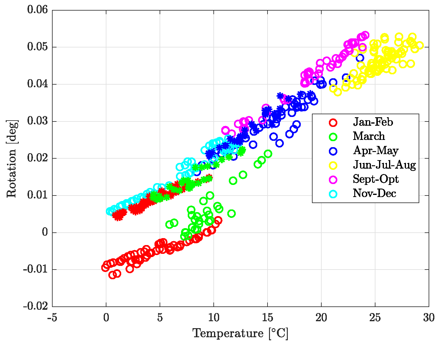
The selection of the periods for training and testing has been corroborated by Figure 8 and Figure 9. In these two figures, the readings of two tiltmeter (T2 and T8) averages per day are plotted against the temperature. Then, the data points are grouped according to months. In Figure 8, the readings of T2 present a transition between January 2021 and April 2021. Then, it looks as if the data points stabilised around a regression line. A similar situation can be observed in Figure 9. The tiltmeter T8 features a longer transition phase, from January 2021 to August 2021, before it settles down around a new regression line. Apparently, it took to the bridge between three and nine months to become stable in a new equilibrium position after the October 2020 flood.
This consideration justifies a partition of the two years of measurements available between the training set (from December 2021 to December 2022), which is used to validate the models as well, and the test set (from December 2020 to November 2021), although, usually, the collection of the training set comes chronologically before the test one. Thus, the following procedure was applied to evaluate the two models (iterative and autoencoder) and establish whether they are able to recognise and quantify the effect of the flood.
1.
The iterative model and the autoencoder introduced in Section 4 are trained on the training set. Then, both the training set and the test set are passed to the two models. The estimated values are then used to compute the residuals (Equations (3) and (5)).
2.
For each sensor, a moving average and a moving standard deviation are applied with a one-week window to evaluate the distributions of residuals in time.
3.
For each month, the mean absolute error (MAE) of the scaled residuals is computed; that is, Equations (3) and (5) are applied before the true values, and the estimations are scaled back to the original range. This allows the evaluation of how the sensors detect unusual behaviours on a comparable scale.
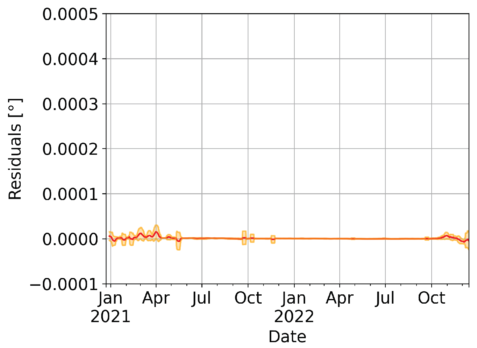
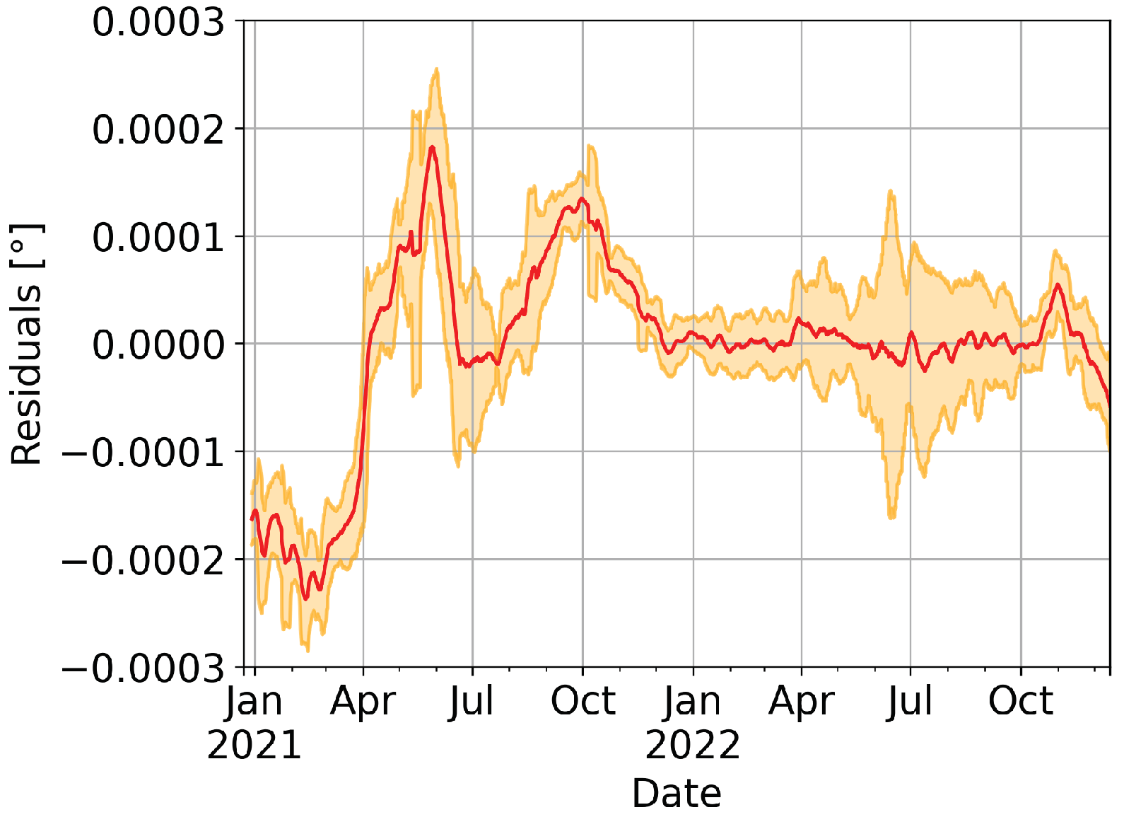
The values obtained during step 2 are computed for both the iterative model and the autoencoder. The results for sensor T1 are plotted in Figure 10 and Figure 11. In red are the mean values, whereas the area in orange refers to a double confidence level ( ± 2 std ). From the figures, one might notice that not only the dispersion of the data for the iterative model is lower, but also the results at the end of 2022 are more consistent compared to those of the autoencoder. In fact, the residual for the AU model has an unexpected deviation at the end of 2022, which does not have any physical reason behind it.
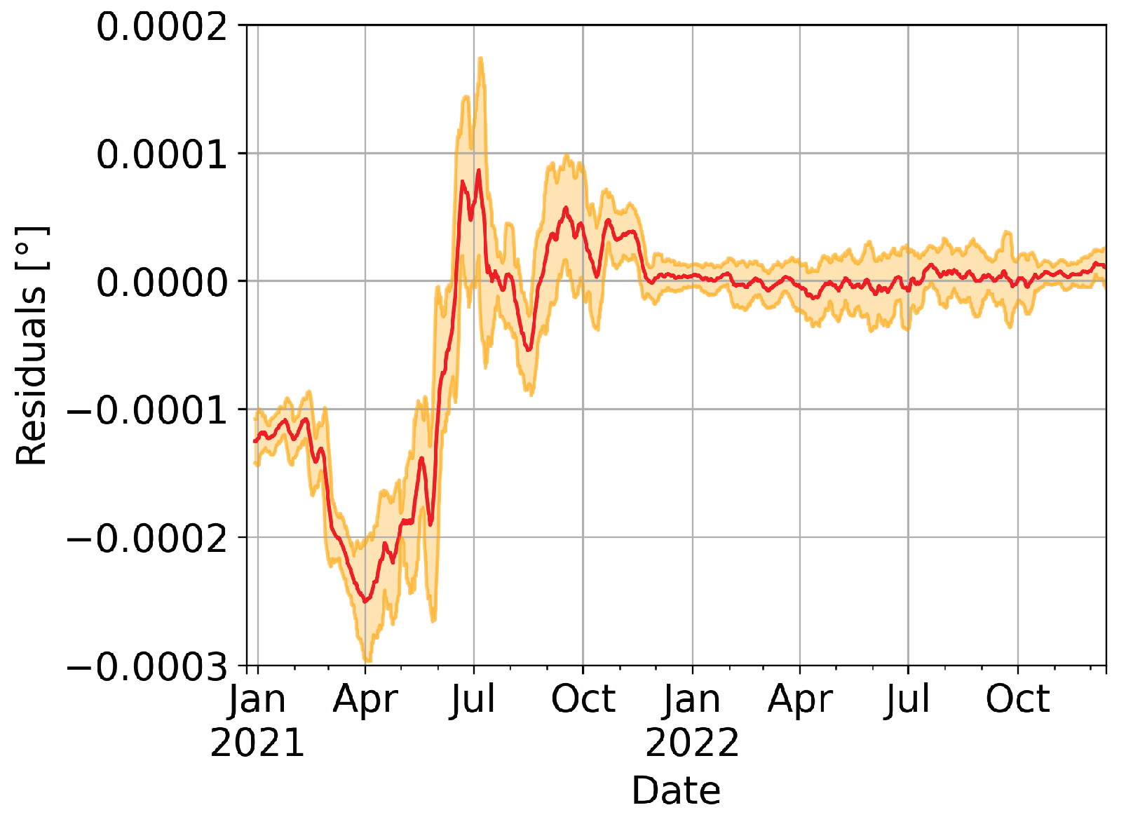
For other sensors, such as T2, the residuals produced by the two models are surprisingly similar (Figure 12 and Figure 13). Likewise, this happens to T3, T4, T7, T8, T9, T12 and T13. For other sensors, such as T10, the iterative model seems to succeed in recognising the flood effects (Figure 14) whereas the autoencoder totally failed (Figure 15).
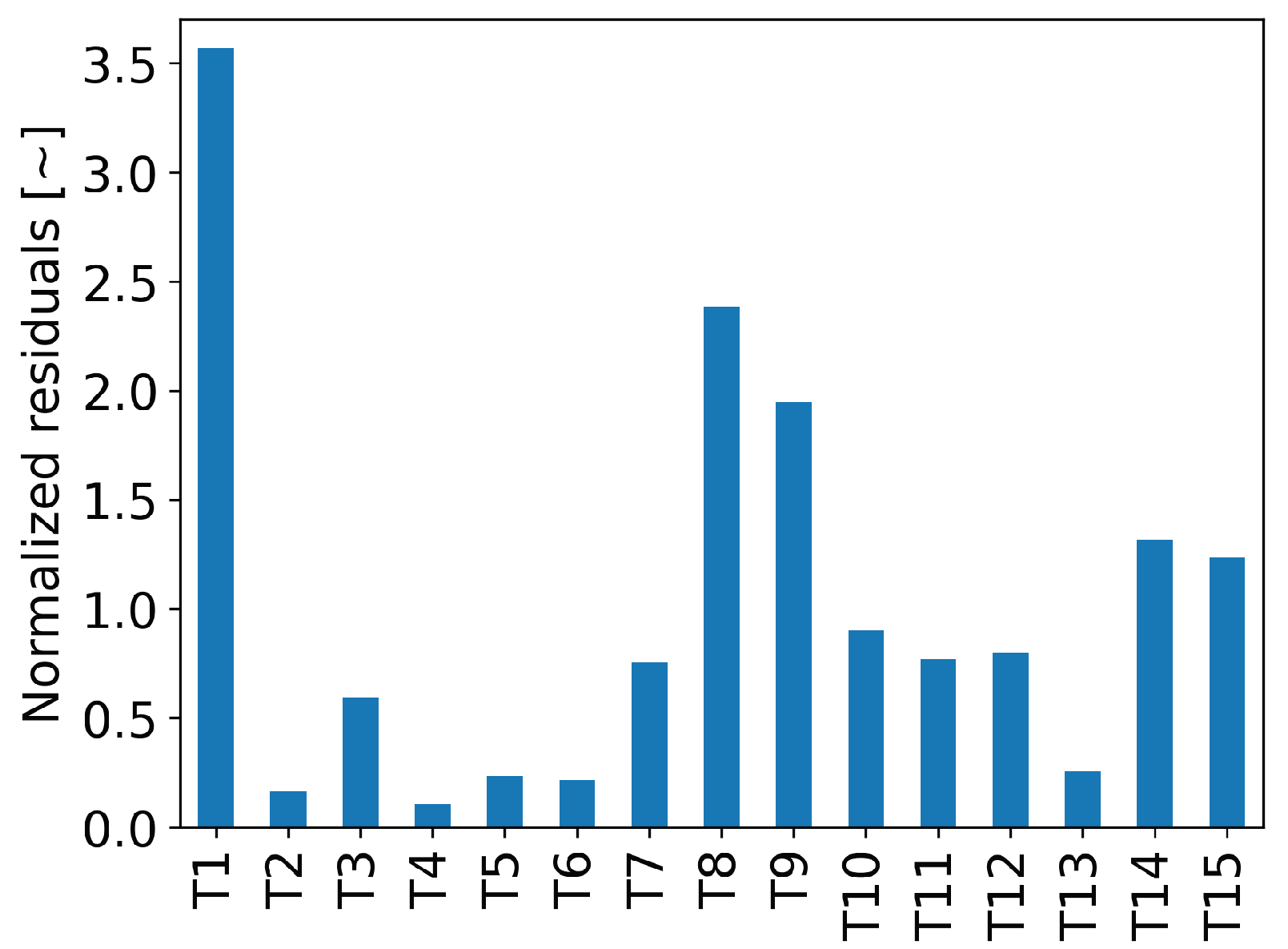
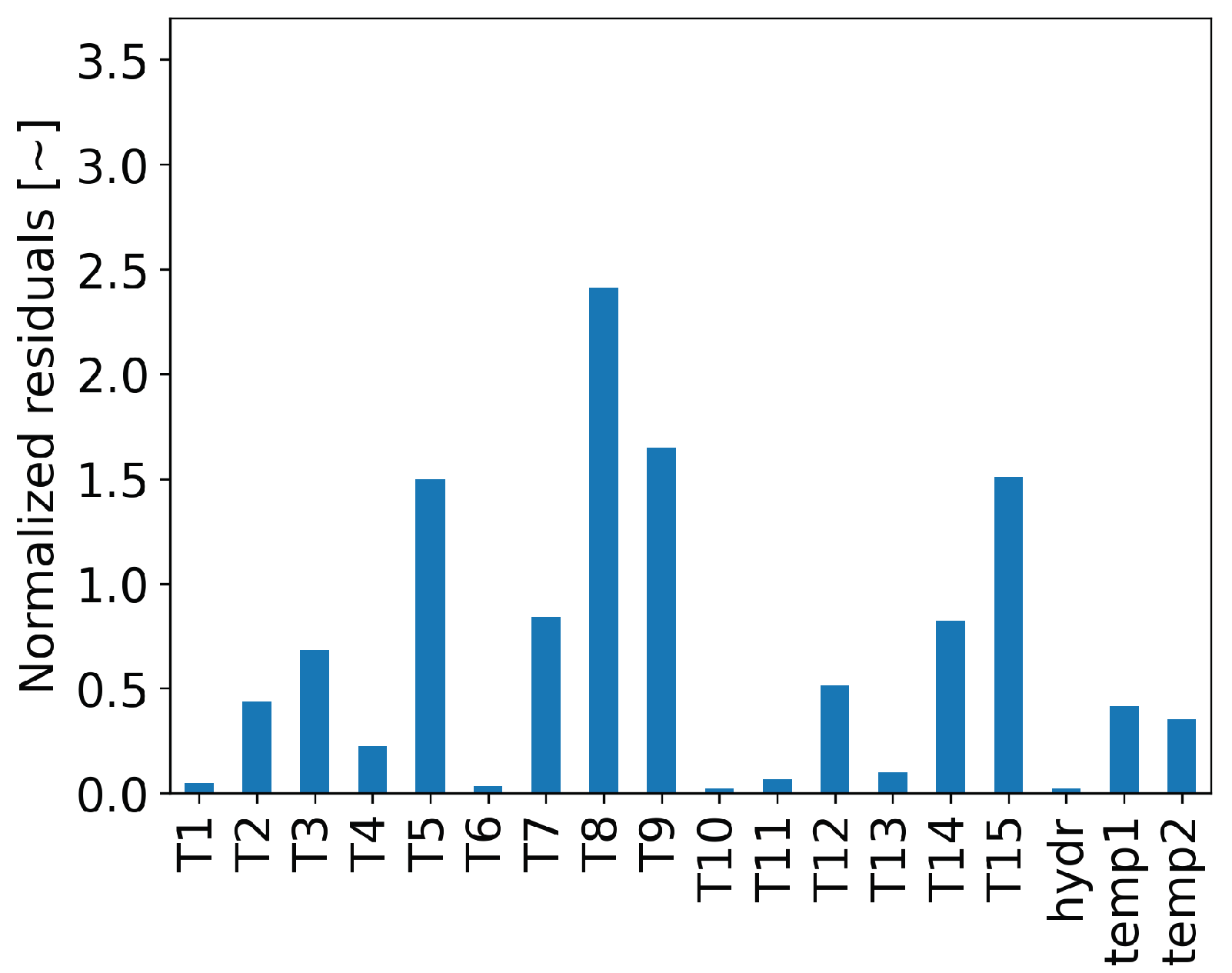
Consistently with step 3, a barplot has been produced for every month and model. Since the residuals are computed before scaling back to the original measurement units, the distributions associated with every sensor (in the training set) have a mean of zero and a variance of one, and, consequently, the results can be compared. For instance, Figure 16 and Figure 17 show the bar plots of MAE for the first month available after the flood (December 2020). The iterative model estimates that strong variations are located at sensors T1, T8 and T9, whereas the situation is practically nominal in T2, T4 and T13, for instance. On the contrary, the autoencoder is less sensitive overall to variations since the scale is even lower.
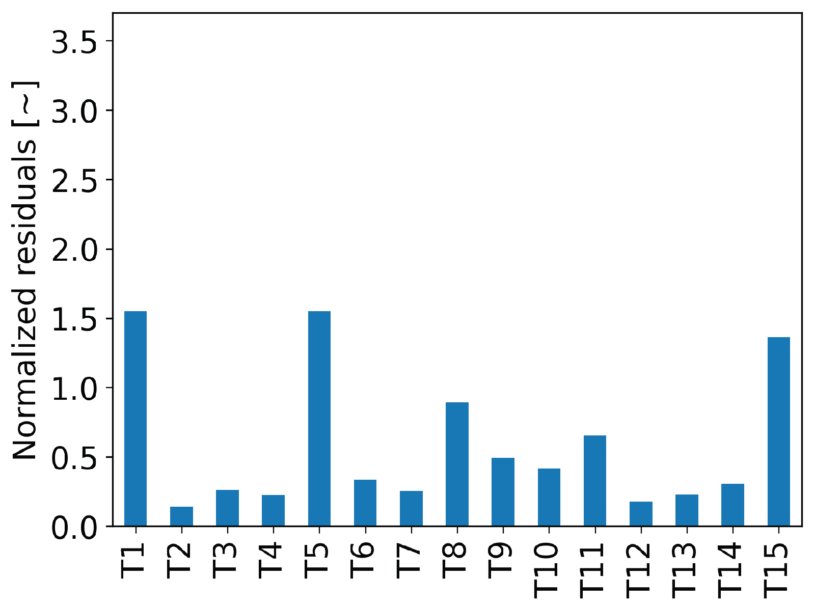
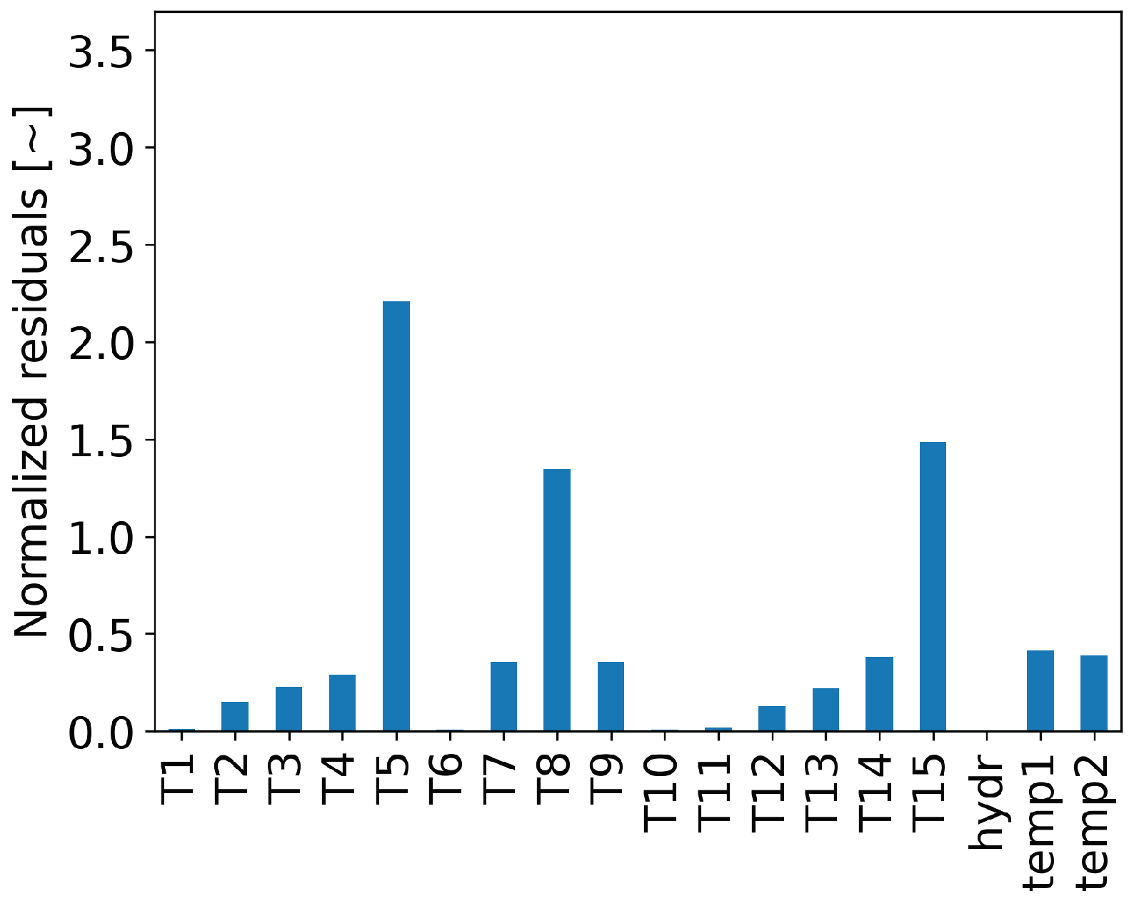
By looking at the later months, the MAE of the residuals rapidly decreases. The month of June is reported in Figure 18 and Figure 19. According to the iterative model, three locations are still far from the new equilibrium condition, which are the ones corresponding to T1, T5 and T15. All of the others residuals have an MAE below one. On the contrary, according to the autoencoder, T1 and other sensors, such as T6, T10 and T11, are already in a perfectly nominal range.
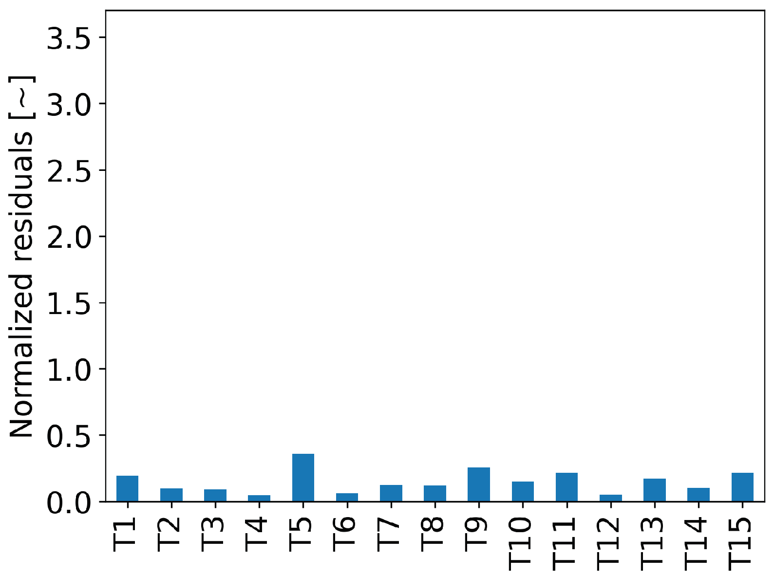
Finally, by looking at the last available month not present in the training set (November 2021, Figure 20 and Figure 21), all of the sensors readings are “normal”, although strong variations among measurements do exist for the autoencoder. In fact, the MAE of sensor T6 is one order of magnitude over T6, and more consistent results are obtained for the iterative model.
Some consideration may be inferred after this comparison between the two anomaly detection systems. The iterative model seems to yield consistent results, whereas it allows for easy quantification of the coherence of sensor readings. For instance, by looking at Figure 8, one might initially think that the region of the bridge closer to sensor 2 settles down around 21 April, but Figure 12 shows that, in April, the T2 residuals go through zero, and then at least two more months were needed for that signal to be coherent with the others. This can also be addressed by the presence of nonlinear activation functions in the neural networks’ layers, which might find a wider variety of relationships rather than just linear ones.
On the contrary, the autoencoder produced similar results for some sensors, whereas, for others, it simply does not yield credible results. Since the methodology is fully data-driven and all of the outputs were scaled, it is hazardous to infer whether this can be corrected by acting on the loss function, for instance, by regularising it. However, it is worth underlining that, since the iterative model counts n sub-models, the training time required for an iterative model is approximately n-times higher than the one required for the autoencoder. Actually, the training of a single iterative model’s neural network is slightly faster than the autoencoder model, since it has one output and fewer weights overall. Then, as a rule of thumb:
t train , IT < n × t train , AU
where n is the number of sensors in the acquisition system.
If the computation resources are not a constraint, the iterative models look promising for assessing the health condition of a structure. They are extremely sensitive to structure variations, and they can effectively recognise which location of the construction is most affected by an extraordinary event. Moreover, they look suitable for evaluating whether the structure comes back to the previous equilibrium position or to a new one.

6. Conclusions

In this work, a novel approach able to detect anomalies in structures has been proposed. It demonstrates a greater robustness with respect to the AU while dealing with extraordinary events (flooding, in this case); the only drawback is that it has a higher computational burden that requires a longer training time. With this approach, it is possible to effectively detect an anomalous condition, quantify the entity of the variation and characterise the severity of the situation. Furthermore, with this model, it is possible to assess whether the structure finds a new equilibrium position and determine the moment at which it is reached. Future developments of this work will concern the deployment of this approach for other structures where exceptional events are recorded as well as the implementation of better regressors, such as dynamic ones.

Author Contributions

Conceptualisation, F.M.B., L.R., S.C., C.S. and G.C.; methodology, F.M.B. and L.R.; software, F.M.B. and L.R.; validation, F.M.B., L.R. and L.B.; formal analysis, L.R.; investigation, F.M.B. and L.R.; resources, F.M.B. and L.R.; data curation, F.M.B. and L.R.; writing—original draft preparation, F.M.B., L.R. and L.B.; writing—review and editing, F.M.B., L.R., L.B. and S.C.; visualisation, F.M.B. and L.R.; supervision, S.C., G.C., C.S. and M.B.; project administration, M.B.; funding acquisition, M.B. All authors have read and agreed to the published version of the manuscript.

Funding

This research received no external funding.

Institutional Review Board Statement

Not applicable.

Informed Consent Statement

Not applicable.

Data Availability Statement

Data are unavailable due to privacy.

Conflicts of Interest

The authors declare no conflict of interest.

Abbreviations

The following abbreviations are used in this manuscript:
ANNArtificial neural network
CNN  Convolutional neural network
AIArtificial intelligence
AUAutoencoder
SHMStructural health monitoring
ReLURectified linear unit
MAEMean absolute error

References

  1. Román, Á.F.G.; Khan, M.S.A.; Kabir, G.; Billah, M.; Dutta, S. Evaluation of interaction between bridge infrastructure resilience factors against seismic hazard. Sustainability 2022, 14, 10277. [Google Scholar] [CrossRef]
  2. Guettala, A.; Abibsi, A. Corrosion degradation and repair of a concrete bridge. Mater. Struct. 2006, 39, 471–478. [Google Scholar] [CrossRef]
  3. Biondini, F.; Frangopol, D.M. Life-Cycle Performance of Deteriorating Structural Systems under Uncertainty: Review. J. Struct. Eng. 2016, 142, F4016001. [Google Scholar] [CrossRef]
  4. Mijalković, S.; Cvetković, V. Vulnerability of critical infrastructure by natural disasters. In National Critical Infrastructure Protection–Regional Perspective; University of Belgrade, Faculty of Security Studies, Institute for Corporative Security Studies: Ljubljana, Belgrade, 2013; pp. 91–102. [Google Scholar]
  5. Kadri, F.; Birregah, B.; Châtelet, E. The Impact of Natural Disasters on Critical Infrastructures: A Domino Effect-based Study. J. Homel. Secur. Emerg. Manag. 2014, 11, 217–241. [Google Scholar] [CrossRef]
  6. Zhang, G.; Liu, Y.; Liu, J.; Lan, S.; Yang, J. Causes and statistical characteristics of bridge failures: A review. J. Traffic Transp. Eng. 2022, 9, 388–406. [Google Scholar] [CrossRef]
  7. Nasr, A.; Björnsson, I.; Honfi, D.; Ivanov, O.L.; Johansson, J.; Kjellström, E. A review of the potential impacts of climate change on the safety and performance of bridges. Sustain. Resilient Infrastruct. 2021, 6, 192–212. [Google Scholar] [CrossRef] [Green Version]
  8. World Meteorological Organization. Weather-Related Disasters Increase over Past 50 Years, Causing More Damage but Fewer Deaths. Available online: https://public.wmo.int/en/media/press-release/weather-related-disasters-increase-over-past-50-years-causing-more-damage-fewer (accessed on 31 January 2021).
  9. Iacovino, C.; Turksezer, Z.; Giordano, P.; Limongelli, M. Comparison of Bridge Inspection Policies in terms of Data Quality. J. Bridge Eng. 2022, 27, 04021115. [Google Scholar] [CrossRef]
  10. Lynch, J.; Farrar, C.; Michaels, J. Structural health monitoring: Technological advances to practical implementations [scanning the issue]. Proc. IEEE 2016, 104, 1508–1512. [Google Scholar] [CrossRef]
  11. Figueiredo, E.; Moldovan, I.; Marques, M. Condition Assessment of Bridges: Past, Present, and Future. A Complementary Approach; Universidade Católica Editora: Lisbon, Portugal, 2013. [Google Scholar]
  12. Ye, X.; Tao, J.; Yun, C. A review on deep learning-based structural health monitoring of civil infrastructures. Smart Struct. Syst. 2019, 24, 567–585. [Google Scholar] [CrossRef]
  13. Jian, X.; Zhong, H.; Xia, Y.; Sun, L. Faulty data detection and classification for bridge structural health monitoring via statistical and deep-learning approach. Struct. Control Health Monit. 2021, 28, e2824. [Google Scholar] [CrossRef]
  14. Bao, Y.; Tang, Z.; Li, H.; Zhang, Y. Computer vision and deep learning–based data anomaly detection method for structural health monitoring. Struct. Health Monit. 2019, 18, 401–421. [Google Scholar] [CrossRef]
  15. Mousavi, M.; Gandomi, A.H. Prediction error of Johansen cointegration residuals for structural health monitoring. Mech. Syst. Signal Process. 2021, 160, 107847. [Google Scholar] [CrossRef]
  16. Ni, F.; Zhang, J.; Noori, M.N. Deep learning for data anomaly detection and data compression of a long-span suspension bridge. Comput. Aided Civ. Infrastruct. Eng. 2020, 35, 685–700. [Google Scholar] [CrossRef]
  17. Mao, J.; Wang, H.; Spencer, B.F., Jr. Toward data anomaly detection for automated structural health monitoring: Exploiting generative adversarial nets and autoencoders. Struct. Health Monit. 2021, 20, 1609–1626. [Google Scholar] [CrossRef]
  18. Limongelli, M.; Gentile, C.; Biondini, F.; di Prisco, M.; Ballio, F.; Zonno, G.; Borlenghi, P.; Bianchi, S.; Capacci, L.; Anghileri, M.; et al. Bridge structural monitoring: The Lombardia regional guidelines. Struct. Infrastruct. Eng. 2022, 1–24. [Google Scholar] [CrossRef]
  19. Worden, K.; Dulieu-Barton, J.M. An overview of intelligent fault detection in systems and structures. Struct. Health Monit. 2004, 3, 85–98. [Google Scholar] [CrossRef]
  20. Entezami, A.; Shariatmadar, H.; Mariani, S. Fast unsupervised learning methods for structural health monitoring with large vibration data from dense sensor networks. Struct. Health Monit. 2020, 19, 1685–1710. [Google Scholar] [CrossRef]
  21. Comanducci, G.; Magalhães, F.; Ubertini, F.; Cunha, Á. On vibration-based damage detection by multivariate statistical techniques: Application to a long-span arch bridge. Struct. Health Monit. 2016, 15, 505–524. [Google Scholar] [CrossRef]
  22. Hu, W.H.; Cunha, Á.; Caetano, E.; Rohrmann, R.G.; Said, S.; Teng, J. Comparison of different statistical approaches for removing environmental/operational effects for massive data continuously collected from footbridges. Struct. Control Health Monit. 2017, 24, e1955. [Google Scholar] [CrossRef]
  23. Huang, J.C.; Ko, K.M.; Shu, M.H.; Hsu, B.M. Application and comparison of several machine learning algorithms and their integration models in regression problems. Neural Comput. Appl. 2020, 32, 5461–5469. [Google Scholar] [CrossRef]
  24. Reynolds, D.A. Gaussian mixture models. Encycl. Biom. 2009, 741. [Google Scholar]
  25. Chen, Z.; Yeo, C.K.; Lee, B.S.; Lau, C.T. Autoencoder-based network anomaly detection. In Proceedings of the 2018 Wireless Telecommunications Symposium (WTS), Phoenix, AZ, USA, 17–20 April 2018; pp. 1–5. [Google Scholar] [CrossRef]
  26. Ahmad, S.; Styp-Rekowski, K.; Nedelkoski, S.; Kao, O. Autoencoder-based condition monitoring and anomaly detection method for rotating machines. In Proceedings of the 2020 IEEE International Conference on Big Data (Big Data), IEEE, Atlanta, GA, USA, 10–13 December 2020; pp. 4093–4102. [Google Scholar]
  27. Bono, F.; Cinquemani, S.; Chatterton, S.; Pennacchi, P. A deep learning approach for fault detection and RUL estimation in bearings. In NDE 4.0, Predictive Maintenance, and Communication and Energy Systems in a Globally Networked World; SPIE: Bellingham, WA, USA, 2022; Volume 12049, pp. 71–83. [Google Scholar]
  28. Shanker, M.; Hu, M.; Hung, M. Effect of data standardization on neural network training. Omega 1996, 24, 385–397. [Google Scholar] [CrossRef]
  29. Dahl, G.E.; Sainath, T.N.; Hinton, G.E. Improving deep neural networks for LVCSR using rectified linear units and dropout. In Proceedings of the 2013 IEEE International Conference on Acoustics, Speech and Signal Processing, IEEE, Vancouver, BC, Canada, 26–31 May 2013; pp. 8609–8613. [Google Scholar]
Figure 1. Candia Bridge Monitoring System.
Futureinternet 15 00119 g001
Figure 2. Data arrangement after preprocessing.
Futureinternet 15 00119 g002
Figure 3. A model (such as a neural network) takes the temperature as the input and gives an estimation of the readings of other sensors.
Futureinternet 15 00119 g003
Figure 4. A model estimates the values of one group of sensors by taking all of the other groups as the input.
Futureinternet 15 00119 g004
Figure 5. Autoencoder structure.
Futureinternet 15 00119 g005
Figure 6. Iterative model’s architecture.
Futureinternet 15 00119 g006
Figure 7. Autoencoder’s architecture.
Futureinternet 15 00119 g007
Figure 8. T2 daily average trend (2021–2022) vs. temperature.
Futureinternet 15 00119 g008
Figure 9. T8 daily average trend (2021–2022) vs. temperature.
Futureinternet 15 00119 g009
Figure 10. Iterative model: T1 residuals.
Futureinternet 15 00119 g010
Figure 11. Autoencoder: T1 residuals.
Futureinternet 15 00119 g011
Figure 12. Iterative model: T2 residuals.
Futureinternet 15 00119 g012
Figure 13. Autoencoder: T2 residuals.
Futureinternet 15 00119 g013
Figure 14. Iterative model: T10 residuals.
Futureinternet 15 00119 g014
Figure 15. Autoencoder: T10 residuals.
Futureinternet 15 00119 g015
Figure 16. Iterative model: bar plots of MAE residuals (December 2020).
Futureinternet 15 00119 g016
Figure 17. Autoencoder: bar plots of MAE residuals (December 2020).
Futureinternet 15 00119 g017
Figure 18. Iterative model: bar plots of MAE residuals (June 2021).
Futureinternet 15 00119 g018
Figure 19. Autoencoder: bar plots of MAE residuals (June 2021).
Futureinternet 15 00119 g019
Figure 20. Iterative model: bar plots of MAE residuals (November 2021).
Futureinternet 15 00119 g020
Figure 21. Autoencoder: bar plots of MAE residuals (November 2021).
Futureinternet 15 00119 g021
Table 1. Channels, sensors and measurement units of the acquisition system mounted on Candia Bridge.
ChannelsSensorsMeasurement Unit
1–15Tiltmetersrad
16Hydrometerm
23, 24Temperatures°C
25Atmospheric pressurebar
26, 27Temperatures°C
28, 29Humidity%
30Wind speedKm/h
31Wind direction°
32Rain ratemm/h
Disclaimer/Publisher’s Note: The statements, opinions and data contained in all publications are solely those of the individual author(s) and contributor(s) and not of MDPI and/or the editor(s). MDPI and/or the editor(s) disclaim responsibility for any injury to people or property resulting from any ideas, methods, instructions or products referred to in the content.