Distributed Average Consensus Algorithms in d-Regular Bipartite Graphs: Comparative Study

Abstract

Consensus-based data aggregation in d-regular bipartite graphs poses a challenging task for the scientific community since some of these algorithms diverge in this critical graph topology. Nevertheless, one can see a lack of scientific studies dealing with this topic in the literature. Motivated by our recent research concerned with this issue, we provide a comparative study of frequently applied consensus algorithms for distributed averaging in d-regular bipartite graphs in this paper. More specifically, we examine the performance of these algorithms with bounded execution in this topology in order to identify which algorithm can achieve the consensus despite no reconfiguration and find the best-performing algorithm in these graphs. In the experimental part, we apply the number of iterations required for consensus to evaluate the performance of the algorithms in randomly generated regular bipartite graphs with various connectivities and for three configurations of the applied stopping criterion, allowing us to identify the optimal distributed consensus algorithm for this graph topology. Moreover, the obtained experimental results presented in this paper are compared to other scientific manuscripts where the analyzed algorithms are examined in non-regular non-bipartite topologies.

1. Introduction

This section, which provides theoretical insight into the subject topic, is divided into five subsections, namely:

☐

Data Aggregation in Multi-Agent Systems: this subsection explains the importance of data aggregation, contains its definition and four-step process, discusses the benefits of its application, provides insight into multi-agent systems (MASs), and justifies the application of data aggregation mechanisms in these systems;

☐

Distributed Consensus-Based Data Aggregation: in this subsection, we explain the general meaning of the term consensus, its meaning in the context of MASs, and the requirements for distributed consensus algorithms;

☐

Theoretical Insight into d-Regular Bipartite Graphs: this subsection provides the definition of d-regular bipartite graphs, their graphical example, and examples of their applications;

☐

Our Contribution: this subsection specifies our contribution presented in this paper and justifies the benefit of this manuscript compared to related papers;

☐

Paper Organization: here, the paper structure is provided.

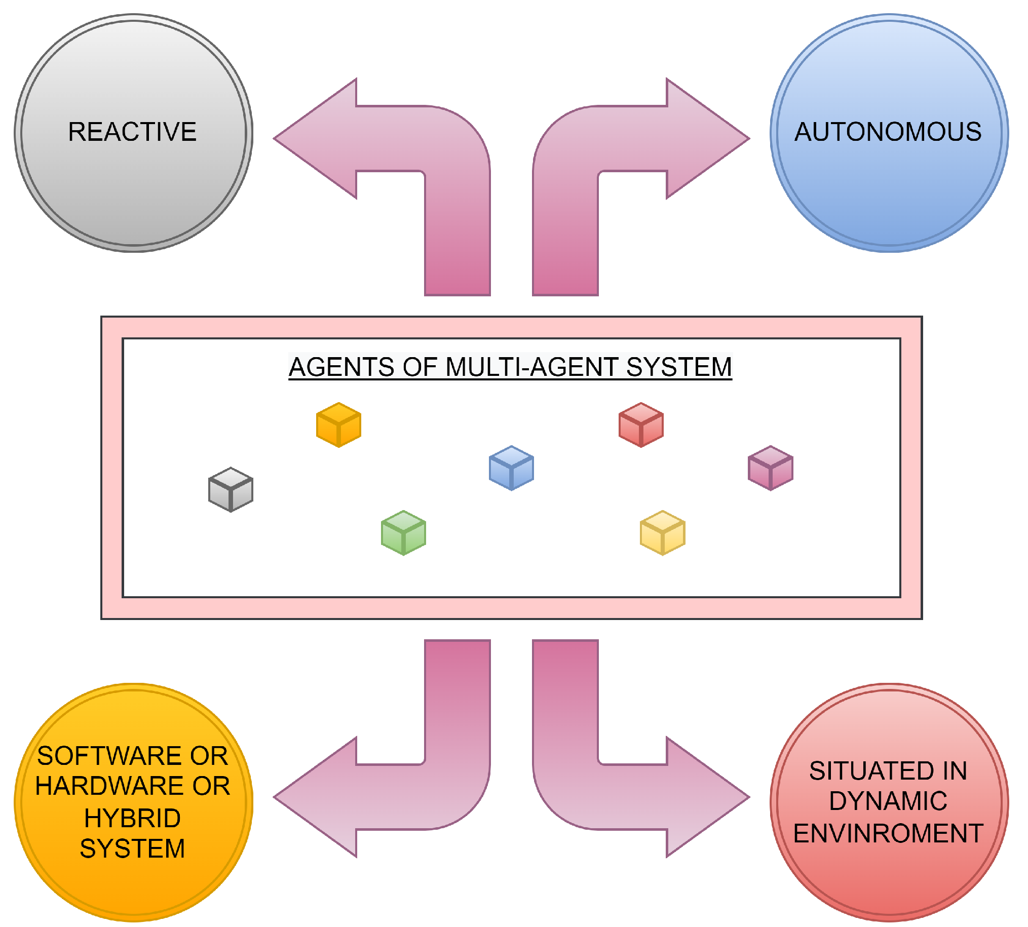
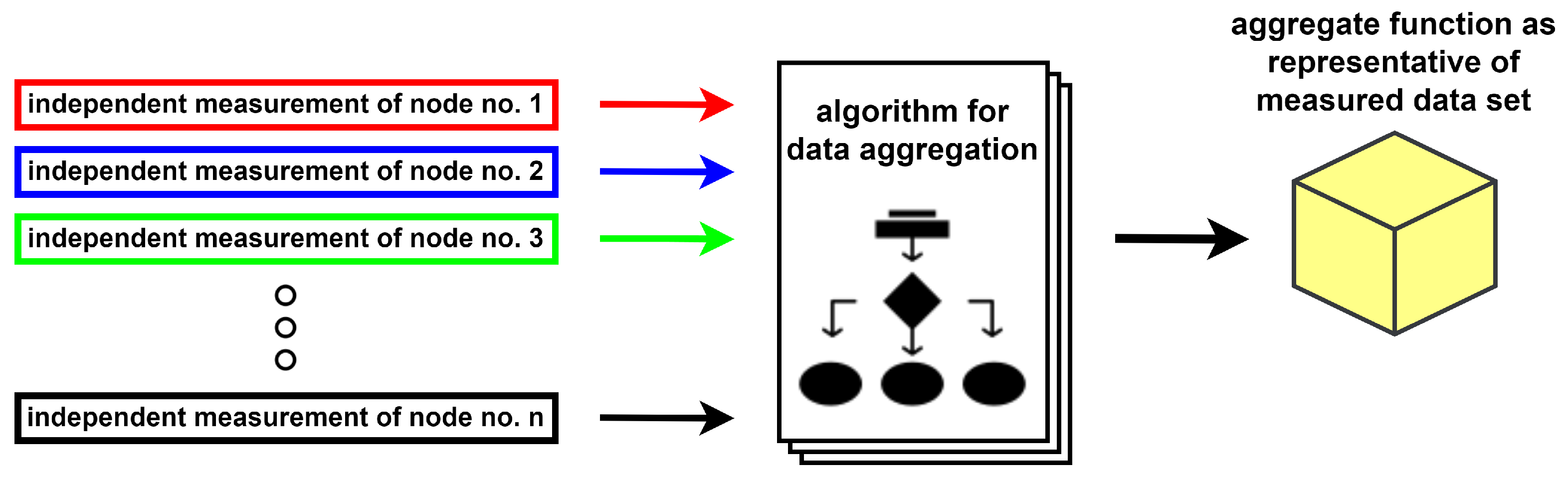
1.1. Data Aggregation in Multi-Agent Systems

How to efficiently combine data from independent information sources is a complicated issue in many contexts [1]. As the data volume around us grows every day, understanding this impenetrable mass of data is becoming an increasingly difficult task in the so-called big data era [2]. Therefore, many experts from various areas have been dealing with this challenge over the last decades [3,4,5,6]. As seen in the literature [7,8,9,10,11], data aggregation seems to be an appropriate technique to organize the mass of raw data in a meaningful manner. In general, one can understand the term data aggregation as a data/information mining process for searching, collecting, and expressing a set of raw data from independent sources in a more transparent and summarized form [12]. In other words, it is a commonplace procedure to simplify various daily processes in our technologically developed era [13]. Data aggregation enables the effective identification of patterns (hard to identify by a common user) in a processed dataset [14]. The final form of aggregated data is conditioned by the purpose that the data are expected to be used for. Generally, the process of data aggregation can be partitioned into four successive phases, namely [15].

■

Phase 1: extracting data from independent sources;

■

Phase 2: storing the extracted data;

■

Phase 3: interpretation of the stored data;

■

Phase 4: presenting the processed data in an appropriate form.

As seen in the literature [16,17,18,19], the application of data aggregation is beneficial in various areas e.g., the financial sector, marketing, medicine, technical industries, etc. In this paper, we consider a group of independent entities (referred to as agents) forming MAS, where data aggregation is exploited in order to optimize the applications executed in these systems in numerous aspects [20]. The agents in these systems are required to communicate with each other and interact with their adjacent environment (see Figure 1 for the characteristic features of agents forming MAS) [11]. The primary task of MASs is to efficiently and quickly solve difficult issues unmanageable for individual solvers. This technology has applications in different areas, e.g., artificial intelligence, monitoring, control, grid computing, military, electronics, manufacturing, etc. [21].

In this paper, we consider a scenario where agents of MAS are expected to independently measure a physical quantity of one’s interest, and an algorithm for aggregating these independent data is subsequently applied in order to determine an appropriate aggregate function from these measured values (see Figure 2 for a general architecture of the data aggregation in this scenario). Thus, data aggregation includes the process of forwarding a summary of measured data instead of all the data. As discussed in [22], the aggregation of sensor-measured values in scenarios such as this one can suppress many negative environmental factors (e.g., pressure variations, temperature, noises, radiation, etc.) whereby the quality of service (QoS) can be significantly optimized in many topical MASs. Moreover, its application can remove highly correlated or even duplicated sensor-measured values and, thus, also optimizes the overall energy consumption.

In this paper, we focus our attention on distributed average consensus algorithms, which represent a frequently applied solution for the aggregation of data in many technologies, e.g., wireless sensor networks, the Internet of Things, blockchains, etc., as shown in [23,24,25].

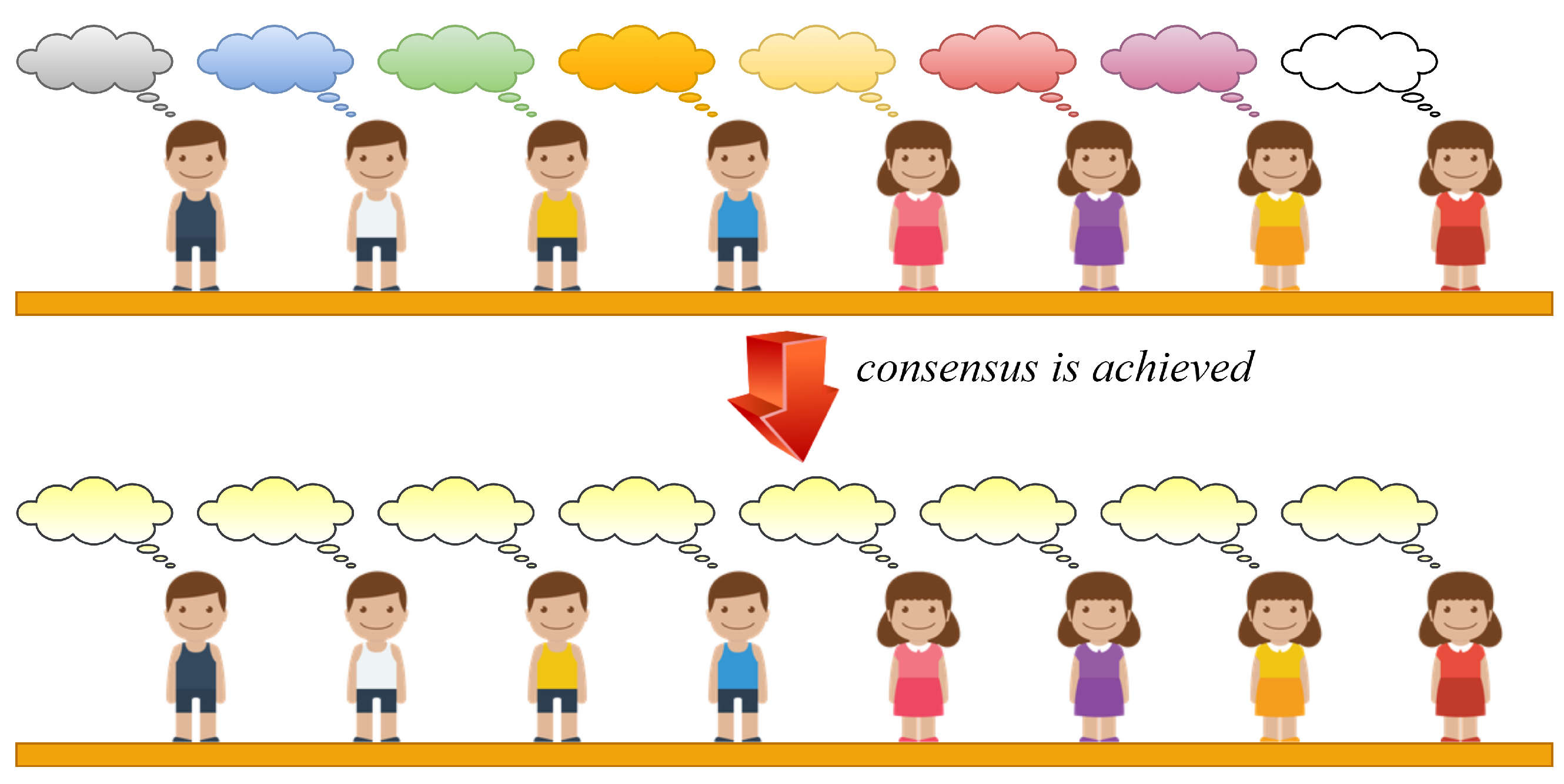
1.2. Distributed Consensus-Based Data Aggregation

The consensus problem is a multi-disciplinary scientific field addressing how to achieve general agreement on some fact among the entities of a given community/group with different attitudes towards this fact [26]. As shown in the literature [27,28,29,30,31,32], the term consensus is applicable in various areas, e.g., cryptocurrencies, economics, bioinformatics, control of unmanned aerial vehicles (UAVs), load balancing, clock synchronization, etc. In Figure 3, we show an example of a group of eight children with and without a consensus on their opinions.

In computer science, the term distributed consensus can be understood as a process of reaching an agreement among the agents of MASs with different initial values on a single data value (for example, arithmetic mean, sum, extreme, etc.) [33]. Simply said, agents of MASs are computerized devices (e.g., wireless sensor nodes) concurrently accomplishing some goals by regularly exchanging necessary information with each other in order to fulfill a specific task [34]. The agents of MASs are able to achieve the consensus only if the same consensus algorithm is followed. As stated in [35,36], a consensus algorithm is required to meet these three conditions (otherwise, the consensus among the agents of MASs cannot be achieved):

■

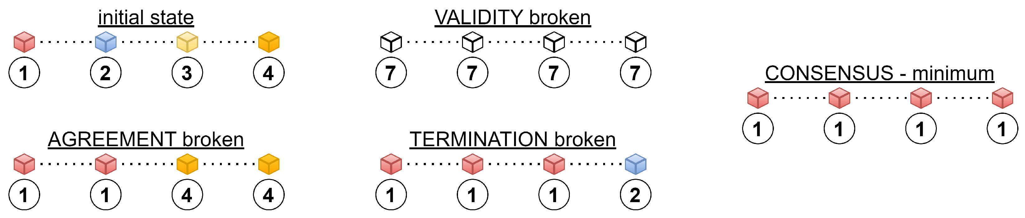
Agreement: all the non-faulty agents of MASs are required to agree on the same value (resp. on a precise estimate of this value);

■

Validity: All the agents of MASs have to agree on a value suggested by the values of these agents. In other words, none of the non-faulty agents in MASs can decide on a value that is not suggested by the value of the agents in the system;

■

Termination: the distributed consensus is achieved, provided that each non-faulty agent in MASs is in the agreement with all the other ones.

In Figure 4, we depict an example of a network with the broken conditions discussed above and the proper execution. Here, we assume that a distributed consensus algorithm for finding the minimum from the measured dataset is applied.

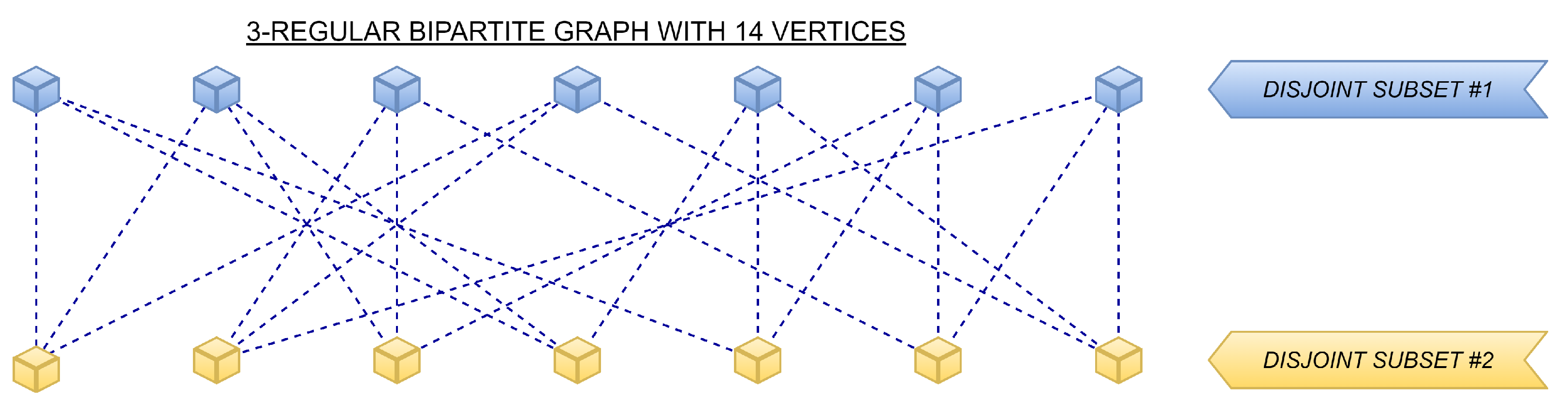
1.3. Theoretical Insight into d-Regular Bipartite Graphs

This subsection is concerned with d-regular bipartite graphs, one of this paper’s primary points of interest. First, let us focus on their definition provided in Definition 1 and their sample topology shown in Figure 5.

Definition 1.

A graph G is said to be d-regular bipartite if [37,38]:

■

Definition of d-regular graphs: the degree of each vertex from V is the same and equal to d;

■

Definition of bipartite graphs: its vertex set V is splittable into two disjoint subsets such that two vertices from the same disjoint subset are not linked to one another.

Thus, d-regular bipartite graphs are a graph type that is regular and bipartite, as seen above. In other words, regular graphs can be understood as graphs with pre-defined degree sequences and gain significant attention in terms of both the practical and theoretical views [39]. Bipartite graphs are graphs where each edge belongs to an odd number of bonds and are also often points of interest. As one can see in the literature [39,40,41], regular bipartite graphs have found applications in various areas and contexts (e.g., finding the perfect matching, quantum machine learning, Poincaréand log-Sobolev inequalities, etc.) over the past decades. As further shown in [42,43,44,45], bipartite graphs are often used in social networks to describe scenarios where a mutual connection exists only between two distinct sets (e.g., supporting learning, majority opinion diffusion, the core–periphery problem, joining a collaboration network, joining a bibliographic network, etc.). As further seen from the papers, regular graphs are also frequently applied in social networks. As shown in [46], regular and irregular bipartite graphs also have applications in biology. The authors of that paper present Nash equilibria for games that are played on these topologies. Moreover, it is discussed in the paper that bipartite graphs can be applied to many interactions, such as plant–animal mutualisms, pollinator webs, seed dispersal, etc. As further seen from [47], regular bipartite graphs also have applications in networks. The authors of that paper apply the Cartesian and tensor product approaches as a tool to decompose bipartite circulant graphs into numerous graph categories. In addition, the application of the mentioned graph types is also seen in other areas such as medicine, linguistics, physics, etc. [48,49,50].

1.4. Our Contribution

As seen in the literature preview, there is a lack of papers concerned with an analysis of distributed consensus algorithms in d-regular bipartite graphs even though this critical graph topology can cause the divergence of an algorithm [51]. As mentioned earlier in this paper, we focus our attention on a comparative study of frequently applied distributed consensus algorithms in randomly generated d-regular bipartite graphs with various connectivities. Namely, we chose the following algorithms for examination:

■

Maximum-Degree weights (MD);

■

Local-Degree weights (LD);

■

Metropolis–Hastings algorithm (MH);

■

Best-Constant weights (BC);

■

Convex Optimized weights (OW);

■

Constant weights (CW);

■

Generalized Metropolis–Hastings algorithm (GMH).

More specifically, we examined these algorithms by applying a common metric for performance evaluation with the assumptions that their execution is bounded by a stopping criterion with various precisions, and the arithmetic mean from the initial inner states of all the agents in MASs was estimated. As identified in our recent paper [52], MD and LD do not converge in d-regular bipartite graphs as the third convergence condition is broken in this topology. However, as shown in [53], the inner states of both algorithms oscillate between two values instead of approaching infinitely high values (as shown in [52], the divergence usually results in the second case). Despite the mentioned divergence, it is, thus, meaningful to also include these two algorithms in our analyses since the consensus can theoretically be achieved due to the mentioned oscillation and the application of a stopping criterion. The primary intention of this paper was to identify the best-performing distributed consensus algorithm and verify whether all the algorithms with bounded execution can achieve the consensus in d-regular bipartite graphs. Moreover, the experimentally obtained results are compared to related papers where these algorithms are examined in non-regular non-bipartite graphs.

1.5. Paper Organization

This paper is organized into six sections, namely:

☐

Section 2—Related Work: this is divided into two subsections and consists of topical and frequently cited papers addressing either consensus-based data aggregation in subjected/closely related graph topologies or the algorithms chosen for evaluation in non-regular non-bipartite graphs;

☐

Section 3—Theoretical Background: this is divided into three subsections and provides the used mathematical model of MASs, a general definition of distributed consensus algorithms, and the weight matrices of the examined distributed average consensus algorithms;

☐

Section 4—Experiments and Discussion: this is formed by three subsections again, consisting of the applied research methodology, experimental results, and a comparison of our conclusions with conclusions presented in papers where the selected algorithms are examined in non-regular non-bipartite graphs;

☐

Section 5—Conclusions: this provides a brief summary of the contribution presented in this paper;

☐

Appendix A—Appendix: this contains tables with the experimental results in numerical form.

2. Related Work

This section consists of two subsections, namely:

☐

Distributed Consensus Algorithms in d-Regular Bipartite Graphs: this subsection introduces papers addressing consensus-based algorithms for data aggregation in regular bipartite graphs and related graphs;

☐

Distributed Consensus Algorithms in non-Regular non-Bipartite Graphs: in this subsection, we provide an overview of papers concerned with a comparison of the chosen algorithms in non-regular non-bipartite graphs.

2.1. Distributed Consensus Algorithms in d-Regular Bipartite Graphs

As shown in the literature, only a few papers are concerned with distributed average consensus algorithms in regular bipartite graphs even though this topology may prevent some of these algorithms from functioning properly.

In [51], the authors examine MD and GMH in this graph topology and identify that both MD and GMH with the optimal mixing parameter (LD) diverge in these graphs. In [52], a novel distributed mechanism for detecting MD in regular bipartite graphs (and ensuring its convergence after reconfiguration) is proposed and examined. In addition, a comprehensive spectral analysis justifying the divergence of the algorithm is provided in that paper. In [53], a comprehensive analysis of MD and GMH with the optimal mixing parameter (LD) is presented. In the paper, it is shown how the inner states oscillate in graphs of various connectivities, and it is further identified that the mean square error of the estimates cannot drop below a certain threshold value. Surprisingly, this threshold value is not conditioned by the graph connectivity, as identified in the paper. The paper [54] is focused on a heterogeneous diffusion-based communication protocol that optimizes the convergence rate of the average consensus algorithm. In that paper, the authors compare their approach with concurrent ones in regular bipartite graphs (not only in this topology) and identify that this approach outperforms other algorithms. As further seen in [55,56,57,58,59,60,61], the authors of these papers assume distributed consensus algorithms in either (only) bipartite, (only) regular, Ramanujan, triangular regular, strongly regular, distance regular, irregular, or disconnected graphs with regular bipartite components. Thus, these papers do not exactly address the same issue as we do in this paper. As shown above, no paper addressing a comparative study of distributed average consensus algorithms in d-regular bipartite graphs can be found in the literature. Therefore, our work represents a significantly novel contribution compared to related work.

2.2. Distributed Consensus Algorithms in Non-Regular Non-Bipartite Graphs

In this section, we turn the readers’ attention to papers dealing with the chosen algorithms for evaluation, in non-regular non-bipartite graphs in this case. This was decided upon in order to compare the conclusion presented in this paper with conclusions valid in non-regular non-bipartite graphs. Thus, our intention was to identify whether there are any differences between the conclusions drawn in non-regular non-bipartite and regular bipartite graphs.

The authors of [62] compared four distributed consensus algorithms (namely, MD, LD, BC, and OW) by applying the asymptotic convergence factor: a commonplace measure to quantify how fast an iterative algorithm converges to the global result, and its associated convergence time. From the presented results, it can be seen that OW performed the best since its values for these two metrics are the lowest (note that a lower value of these metrics indicates that an algorithm was performed better). As further identified in this study, BC was the second-best-performing, LD was the third, and MD achieved the worst performance. The paper [63] is concerned with a comparison of MD, MH, BC, and OW in symmetric, complete-cored symmetric, and K-cored symmetric star topologies by applying several various metrics. The authors of this paper assume that the execution of the algorithm was affected by quantization noise. From the presented results, it is apparent that the OW was faster than the concurrent approaches, but not necessarily with the lowest error (also, BC’s error was high). In general, the worst performance was observed to be achieved by MH in terms of the number of iterations for consensus. The second-best-performing algorithm was MD, and BC was classified as the third-best algorithm among the examined ones. Furthermore, it can be seen that only MD achieved consensus in all the performed scenarios, but other approaches were also able achieve consensus in the overwhelming majority of the scenarios. The authors of [64] show that OW achieved the best performance in the asymptotic phase; meanwhile, LD was considered to be superior in the transient phase. These identified facts allowed the authors of that paper to blend these algorithms via signal-adaptive morphing coefficients. In [51], CW and GMH with various mixing parameters were examined. In these papers, it was observed that higher values of $ϵ$ resulted in a higher performance of the algorithm in the case of CW. In contrast, GMH achieved higher performance, provided that $ϵ$ produced lower values (for $ϵ$ = 0, the algorithm performed the best). In [65], the performance of MD, MH, LD, BC, and OW was evaluated in random geometric graphs, in which the algorithms were applied to estimate the network size. From the presented results, it can be seen that OW performed the best in terms of the asymptotic convergence factor and its associated time, as also identified in [62]. In terms of the number of iterations required for consensus, OW outperformed its concurrent approaches in almost all of the examined scenarios. Only when the precision of the applied stopping criterion was low, and the best-connected entity was selected as the leader, was LD the best-performing algorithm among the studied ones. The worst performance was, in general, observed in the case of MD. In general, BC achieved an average performance, as shown in the figures. If the best-connected entity was selected as the leader, both OW and BC showed low estimation precision in the transient phase. In addition, it is shown that a higher precision of the stopping criterion led to a deceleration in every algorithm. Similarly, in [66], OW outperformed all the other approaches if the algorithms were applied for distributed summing in random geometric graphs and random graphs with various connectivities. This algorithm only achieved lower performance in the early phases in sparsely connected graphs, where it was outperformed by LD. In general, LD also showed high performance in all the examined scenarios (even though it was not as good as OW). The worst performance was achieved by MD, similar to the previous paper. Moreover, one can see from the presented results that an increase in graph connectivity caused all the algorithms to accelerate. As further seen in [67,68,69,70], OW outperformed concurrent approaches in various scenarios and by applying different metrics for performance evaluation. Thus, this algorithm was the best-performing approach in non-regular non-bipartite graphs, as identified in numerous papers.

3. Theorethical Background

This section is divided into three subsections:

☐

Applied Mathematical Model of Multi-Agent Systems: this subsection is concerned with the applied mathematical model of MASs;

☐

General Definition of Average Consensus Algorithms: here, we provide general update rules of distributed average consensus algorithms and their convergence conditions;

☐

Examined Distributed Consensus Algorithms: in this subsection, we introduce all the algorithms chosen for evaluation in d-regular bipartite graphs.

3.1. Applied Mathematical Model of Multi-Agent Systems

In this paper, we model MASs as simple finite undirected unweighted graphs determined by the vertex set V and the edge set E (i.e., G = (V,E)) [71,72]. We assume that both sets are of finite size and time-invariant in our experiments. The first set (V) contains all the graph vertices (each with a unique index), which represent agents in MASs (i.e., V = {v${}_1$, v${}_2$, … v${}_n$,}). The cardinality of V (∣V∣) is determined by the graph order n or, in other words, by the size of MAS. The edge set E consists of all the graph edges, which are direct connections between two vertices (i.e., the distance between two vertices is one hop, and these two nodes are referred to as neighbors). An edge linking v${}_i$ and v${}_j$ is unique and labeled as e${}_{ij}$ later in this paper. The parameter d${}_i$ represents the degree of v${}_i$, which is the number of all the edges incident to v${}_i$. The maximum degree of G is labeled as [73]:

$$\Delta =\underset{i}{max}\left\{d_i\right\}$$

(1)

In the spectral graph theory, there are many useful tools to describe graph connectivity, as seen in [74,75]. One of the most common is the Laplacian matrix L: a diagonally symmetric squared matrix with n${}^2$ entries that is defined as follows [76]:

$${\left[\mathit{L}\right]}_{ij}=\left\{\begin{array}{cc}-1,\hfill & \mathit{if}{\mathit{e}}_{\mathit{ij}}\in \mathit{E}\hfill \\ {\mathit{d}}_i,\hfill & \mathit{if}i=j\hfill \\ 0,\hfill & \mathrm{otherwise}\hfill \end{array}\right.$$

(2)

As shown in [77], many relevant graph properties can be easily studied via the Laplacian spectrum (i.e., via the Laplacian eigenvalues and eigenvectors). The Laplacian spectrum is formed by a set of n eigenvalues sorted in descending order as follows:

$$SPEC\left(\mathbf{L}\right)=\{{\lambda }_1\left(\mathbf{L}\right),{\lambda }_2\left(\mathbf{L}\right),...,{\lambda }_{n-1}\left(\mathbf{L}\right),{\lambda }_n\left(\mathbf{L}\right)\}$$

(3)

Here, ${\lambda }_1$($\mathbf{L}$) is the largest Laplacian eigenvalue, while, ${\lambda }_{n-1}$($\mathbf{L}$) represents the second smallest eigenvalue of the Laplacian spectrum and is known as the algebraic connectivity of G.

As mentioned earlier, we analyzed the chosen algorithms in d-regular bipartite graphs—see Figure 5 for an example of a 3-regular bipartite graph and Definition 1 for their definition.

3.2. General Definition of Average Consensus Algorithms

Average consensus is an essential issue in designing suitable algorithms for distributed computing [70]. Over the past decades, average consensus algorithms have been widely applied in many distributed systems in order to accomplish various computing and controlling tasks [78]. The principle of the mentioned algorithms is based on regular communication among the agents forming MAS and updating their inner states according to neighbors’ information. The primary purpose of these algorithms is to estimate the arithmetic mean from the initial inner states of all the agents in MAS, but they can also be applied for other tasks after tiny modifications (sum estimation, network size estimation) [65,66]. The agents in MAS executing a distributed average consensus algorithm are required to initiate their inner states with a scalar value (e.g., a local sensor-measured value) and exchange their inner states with their adjacent agents in an iterative manner [79]. More specifically, the agents regularly exchange their current inner state with their neighbors and determine the inner state for the next iteration by applying the update rule expressible (from a global view) as the difference Equation (4) [70].

$$\mathbf{x}(\mathit{k}+1)=\mathbf{W}\mathbf{x}\left(\mathit{k}\right)$$

(4)

Here, x(k) is a column variant vector formed by the inner states of all the agents in MAS at k-th iteration. The value of k = 0 represents the initial inner states. W is the weight matrix of an algorithm whose spectrum is defined as follows [52]:

$$SPEC\left(\mathbf{W}\right)=\{{\lambda }_1\left(\mathbf{W}\right),{\lambda }_2\left(\mathbf{W}\right),...,{\lambda }_n\left(\mathbf{W}\right)\}$$

(5)

Similar to the Laplacian spectrum, ${\lambda }_1\left(\mathbf{W}\right)$ refers to the largest eigenvalue of the weight matrix W, ${\lambda }_2\left(\mathbf{W}\right)$ represents its second largest eigenvalue, and ${\lambda }_n\left(\mathbf{W}\right)$ is its smallest eigenvalue. Distributed consensus algorithms differ from each other by the entries of this matrix. As discussed in the mentioned paper, the weight matrix W conditions many algorithm aspects such as the convergence/the divergence, the convergence rate, the robustness to potential threads, the distortion of the final estimates caused by various noises, etc.

From a local view, the difference equation from (4) can be reformulated as follows [62]:

$${\mathit{x}}_i(k+1)=\sum _j^n{\left[\mathbf{W}\right]}_{ij}{\mathit{x}}_j\left(k\right)\phantom{..}for\phantom{.}\forall {\mathit{v}}_i\in \mathbf{V}$$

(6)

As further stated, the average consensus algorithms operate properly, provided that the limit (7) exists.

$$\underset{k\to \infty }{lim}\mathbf{x}\left(\mathit{k}\right)=\underset{k\to \infty }{lim}{\mathbf{W}}^{\mathit{k}}\mathbf{x}\left(0\right)=\frac{1}{\mathit{n}}\mathbf{1}{\mathbf{1}}^{\mathrm{T}}\mathbf{x}\left(0\right)$$

(7)

Here, 1 is an all-ones vector, whose entries are all equal to one, and 1${}^{\mathrm{T}}$ represents its transpose [52]. The existence of this limit means that all the inner states asymptotically converge to the value of the wanted aggregated function. Thus, a precise estimate of (for example) the arithmetic mean from the initial inner states of all the agents in MASs can be obtained by applying distributed consensus algorithms. As identified in [62], meeting the three convergence conditions provided in (8)–(10) guarantees that this limit is sure to exist.

$${\mathbf{1}}^{\mathrm{T}}\mathbf{W}={\mathbf{1}}^{\mathrm{T}}$$

(8)

$$\mathbf{W}\mathbf{1}=\mathbf{1}$$

(9)

$$\rho \left(\mathbf{W}-\frac{1}{\mathit{n}}\mathbf{1}{\mathbf{1}}^{\mathrm{T}}\right)<1$$

(10)

The parameter $\rho$ is a spectral radius, i.e., the largest eigenvalue in the magnitude of the corresponding matrix (see (11)) [80].

$$\rho (·)=\underset{i}{max}\{\mid {\lambda }_i(·)\mid :i=1,2,...n\}$$

(11)

3.3. Examined Distributed Consensus Algorithms

In this subsection, we introduce seven distributed consensus algorithms (also referred to as weights) chosen for evaluation in d-regular bipartite graphs. The selection of these algorithms is justified by the fact that they have probably been the most frequently quoted algorithms in their category over the past decades.

The first examined algorithm is MD, which is frequently applied and has easily implementable weights with the Perron matrix [81]. Thus, all its non-diagonal entries are equal to either zero or the mixing parameter $ϵ$ (i.e., the inverted value of the maximum degree of a graph $\Delta$ in this case). Mathematically, their weight matrix W can be, thus, expressed as follows:

$${\left[\mathit{W}\right]}_{ij}=\left\{\begin{array}{cc}\frac{1}{\Delta },\hfill & \mathit{if} {\mathit{e}}_{\mathit{ij}}\in \mathit{E}\hfill \\ 1-\frac{d_i}{\Delta },\hfill & \mathit{if} \mathit{i}=\mathit{j}\hfill \\ 0,\hfill & \mathrm{otherwise}\hfill \end{array}\right.$$

(12)

As identified in our previous manuscript [52], both the largest ${\lambda }_1$(W) and the smallest eigenvalue ${\lambda }_n$(W) of the weight matrix W are always located on the unit circle in d-regular bipartite graphs if (12) is applied. Furthermore, it is mathematically proven in our previous paper that all the other eigenvalues of the weight matrix W, except for the two previously mentioned ones, are situated inside the unit circle. These facts cause the algorithm to diverge (as the third convergence condition is broken) in such a way that the values of the inner states oscillate between two values (more specifically, between values approaching the averaged initial inner states of the agents forming both the disjointed subsets). Further details about the divergence of MD in regular bipartite graphs can be found in the mentioned manuscript.

In Figure 6, we depict the evolution of the inner state of one of the agents forming MAS in both a regular bipartite/non-regular non-bipartite graph if MD is applied. As seen, the inner state settles down in a non-regular non-bipartite graph; however, it oscillates in the other case.

Another analyzed algorithm is LD, or, in other words, GMH with the optimal mixing parameter (i.e., $ϵ$ = 0). As identified in [51], the weight matrix W of this algorithm is identical to the weight matrix W of MD in d-regular bipartite graphs, whereby this algorithm also diverges in this critical graph topology. See (13) for its weight matrix W [62].

$${\left[\mathit{W}\right]}_{ij}=\left\{\begin{array}{cc}\frac{1}{max\{d_i,d_j\}},\hfill & \mathrm{if}{\mathit{e}}_{ij}\in \mathbf{E}\hfill \\ 1-\sum _{j^{{}^{\prime }}}{\left[\mathit{W}\right]}_{i{j}^{{}^{\prime }}},\hfill & \mathrm{if}i=j\hfill \\ 0,\hfill & \mathrm{otherwise}\hfill \end{array}\right.$$

(13)

In this paper, we also chose MH developed by Metropolis and Hastings et al., which is known as one of the most common Markov Chain Monte Carlo methods to sample a probability distribution in complicated scenarios [70,82]. As further seen, this scheme has found a wide range of applications as a data aggregation mechanism over the last decades. Note that the weight matrix W of this algorithm is identical to the weight matrix W of GMH with the mixing parameter $ϵ$ = 1 [51]. Mathematically, its weight matrix W is defined as follows:

$${\left[\mathit{W}\right]}_{ij}=\left\{\begin{array}{cc}\frac{1}{max\{d_i,d_j\}+1},\hfill & \mathrm{if}{\mathit{e}}_{ij}\in \mathbf{E}\hfill \\ 1-\sum _{j^{{}^{\prime }}}{\left[\mathit{W}\right]}_{i{j}^{{}^{\prime }}},\hfill & \mathrm{if}i=j\hfill \\ 0,\hfill & \mathrm{otherwise}\hfill \end{array}\right.$$

(14)

Another examined algorithm is BC, which is an approach with the Perron matrix based on Laplacian eigenvalues. Theoretically, these weights are considered to be the fastest algorithm among those with the Perron Matrix, and their weight matrix W is defined as [83]:

$${\left[\mathit{W}\right]}_{ij}=\left\{\begin{array}{cc}\frac{2}{{\lambda }_1\left(\mathbf{L}\right)+{\lambda }_{n-1}\left(\mathbf{L}\right)},\hfill & \mathrm{if}{\mathit{e}}_{ij}\in \mathbf{E}\hfill \\ 1-d_{\mathit{i}}\frac{2}{{\lambda }_1\left(\mathbf{L}\right)+{\lambda }_{n-1}\left(\mathbf{L}\right)},\hfill & \mathrm{if}i=j\hfill \\ 0,\hfill & \mathrm{otherwise}\hfill \end{array}\right.$$

(15)

We also included OW in our analyses and experiments. In general, OW is the best-performing algorithm among the distributed consensus algorithms [62]. These weights are, therefore, often referred to as the fastest distributed linear averaging algorithm and are designed in such a way that their weight matrix W is optimized according to eigenvalues, i.e.:

$$\begin{array}{ccc}\mathrm{minimize}\hfill & \hfill & \hfill \rho (\mathbf{W}-\frac{1}{\mathit{n}}\mathbf{1}{\mathbf{1}}^{\mathrm{T}})=max\{{\lambda }_2\left(\mathbf{W}\right),-{\lambda }_n\left(\mathbf{W}\right)\}\\ \mathrm{subject}\mathrm{to}\hfill & \hfill & \hfill \mathbf{W}\in \mathbf{S},{\mathbf{1}}^{\mathrm{T}}\mathbf{W}={\mathbf{1}}^{\mathrm{T}},\mathbf{W}\mathbf{1}=\mathbf{1}\end{array}$$

(16)

Here, $\mathbf{W}\in \mathbf{S}$ represents the constraint on the sparsity pattern of the weight matrix W, where S is defined as follows:

$$\begin{array}{c}\hfill \mathbf{S}=\{\mathbf{W}\in {\mathbf{R}}^{n\times n}\mid {\left[W\right]}_{ij}=0\mathrm{if}\{i,j\}\notin \mathbf{E}\mathrm{and}i\ne j\}\end{array}$$

(17)

In this paper, we also examine CW, an approach with the Perron matrix provided in (18), where the mixing parameter $ϵ$ takes value from the interval (19) [51]:

$${\left[\mathbf{W}\right]}_{ij}=\left\{\begin{array}{cc}ϵ,\hfill & \mathrm{if}e{}_{ij}\in \mathbf{E}\hfill \\ 1-d_iϵ,\hfill & \mathrm{if}i=j\hfill \\ 0,\hfill & \mathrm{otherwise}\hfill \end{array}\right.$$

(18)

$$0<ϵ<\frac{1}{\Delta }$$

(19)

The last investigated algorithm is GMH, whose weight matrix W is defined as (20) [51]. Its mixing parameter $ϵ$ is a variable again, taking the values from (21):

$${\left[\mathbf{W}\right]}_{ij}=\left\{\begin{array}{cc}\frac{1}{max\{d_i,d_j\}+ϵ},\hfill & \mathrm{if}{\mathit{e}}_{ij}\in \mathbf{E}\hfill \\ 1-\sum _{j^{{}^{\prime }}}{\left[\mathit{W}\right]}_{i{j}^{{}^{\prime }}},\hfill & \mathrm{if}i=j\hfill \\ 0,\hfill & \mathrm{otherwise}\hfill \end{array}\right.$$

(20)

$$0\le ϵ\le 1$$

(21)

At the end of this subsection, we provide the spectrum of the weight matrix W for all the examined algorithms in 3-regular bipartite graphs with n = 30. As seen from Figure 7, the smallest eigenvalue ${\lambda }_n\left(\mathbf{W}\right)$ of the weight matrix W is greater than minus one for each examined algorithm, except MD and LD, as stated above in this paper.

4. Experiments and Discussion

This section is organized as follows:

☐

Research Methodology and Applied Metric for Performance Evaluation: in this subsection, we introduce the simulation tool used, we specify the used d-regular bipartite graphs, and we provide the applied metric, the used stopping criterion, the method of generating the initial inner states, and the examined setups of CW and GMH;

☐

Experimental Results and Discussion about Observable Phenomena: this subsection consists of the experimentally obtained results depicted in 15 figures and a subsequent discussion;

☐

Comparison with Papers Concerned with Examined Algorithms in Non-Regular Non-Bipartite Graphs: here, we compare the contributions presented in this paper with manuscripts addressing the examined algorithms in non-regular non-bipartite graphs.

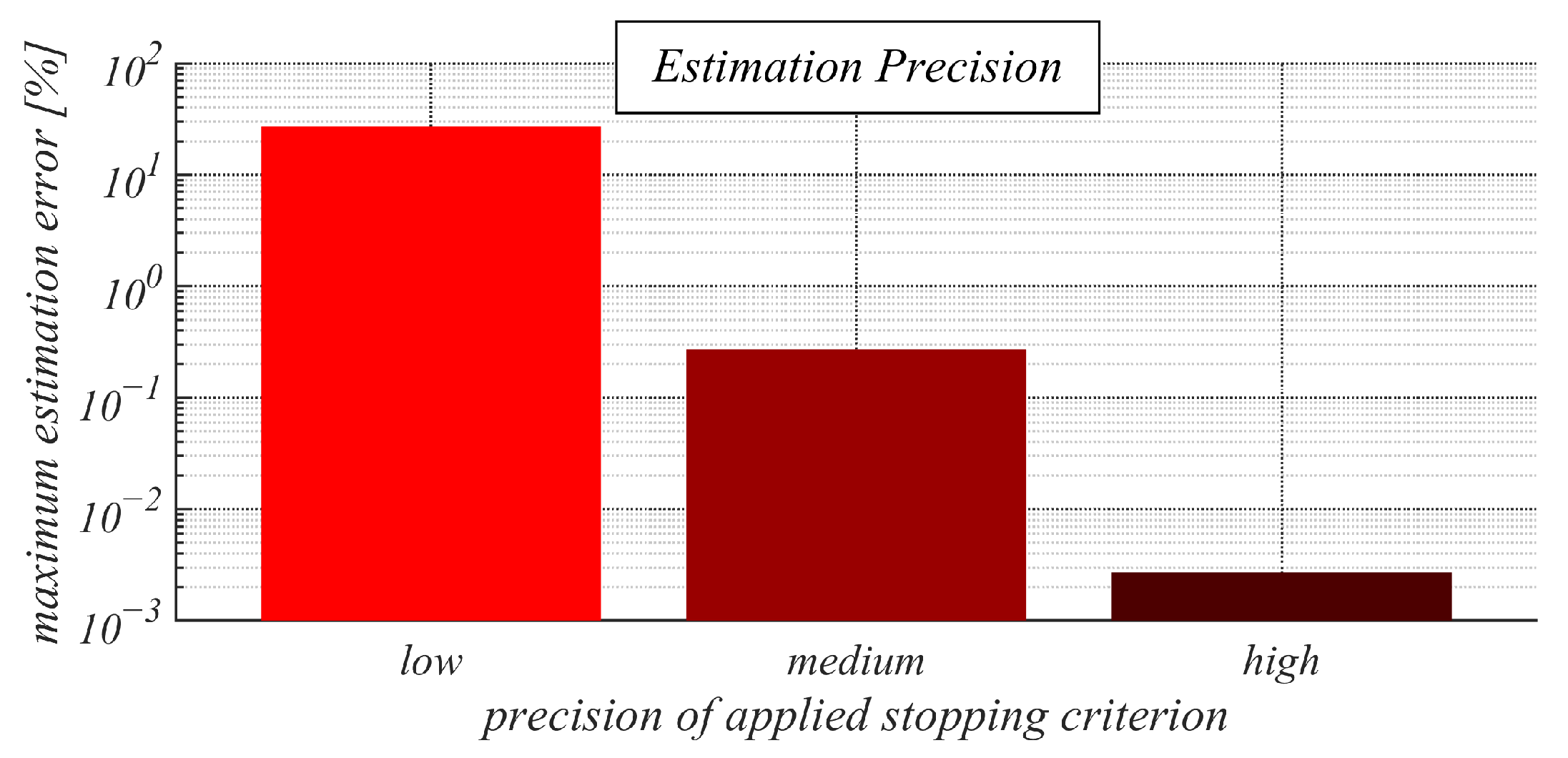
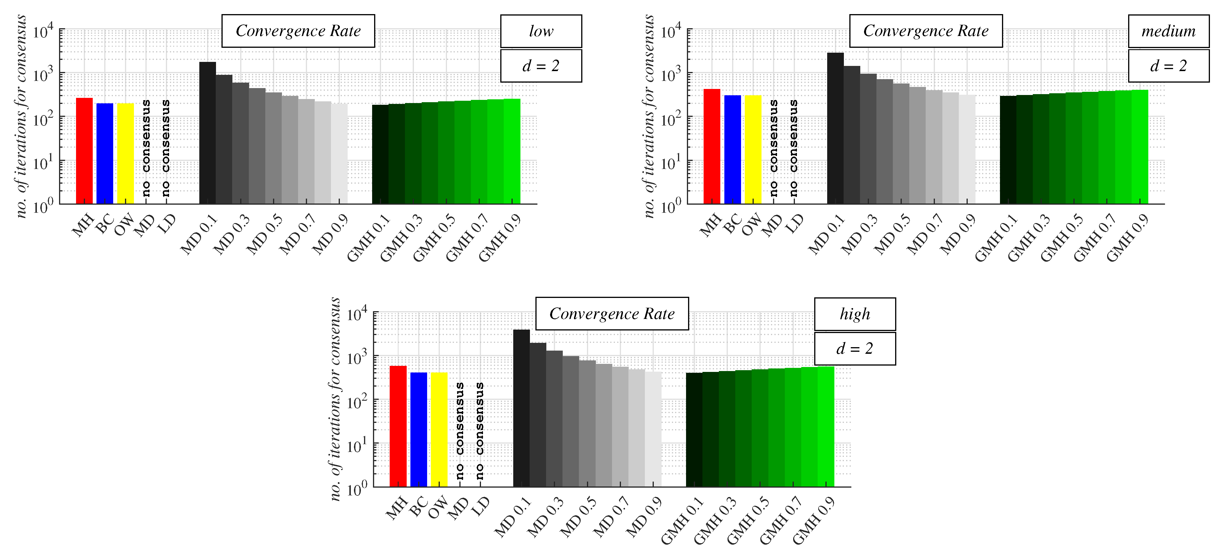
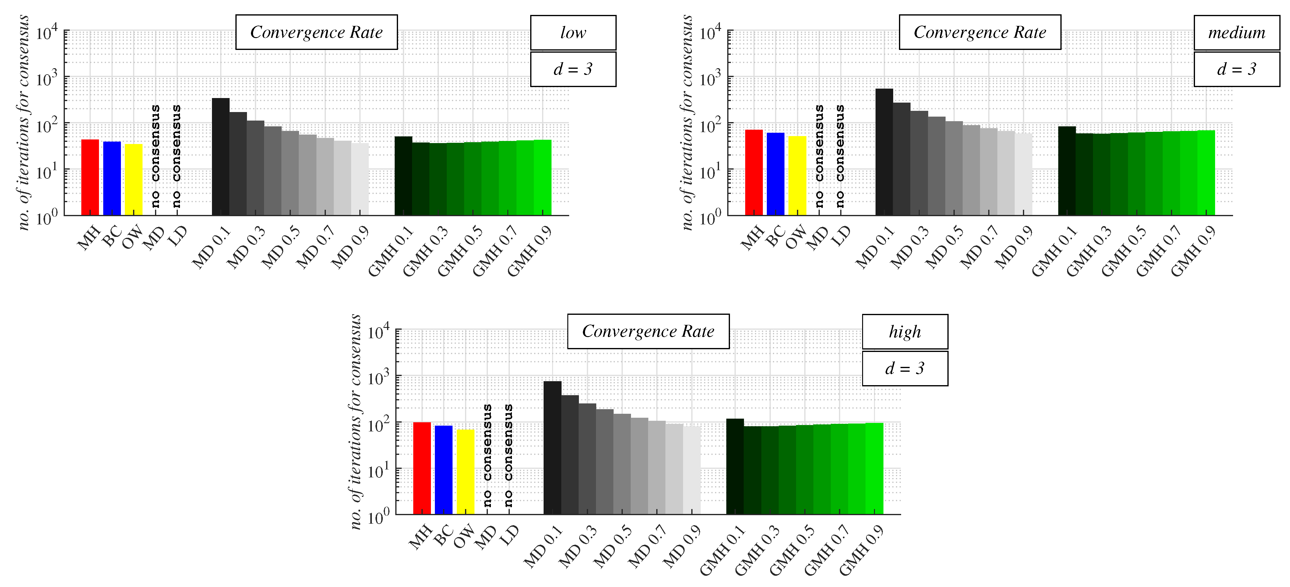
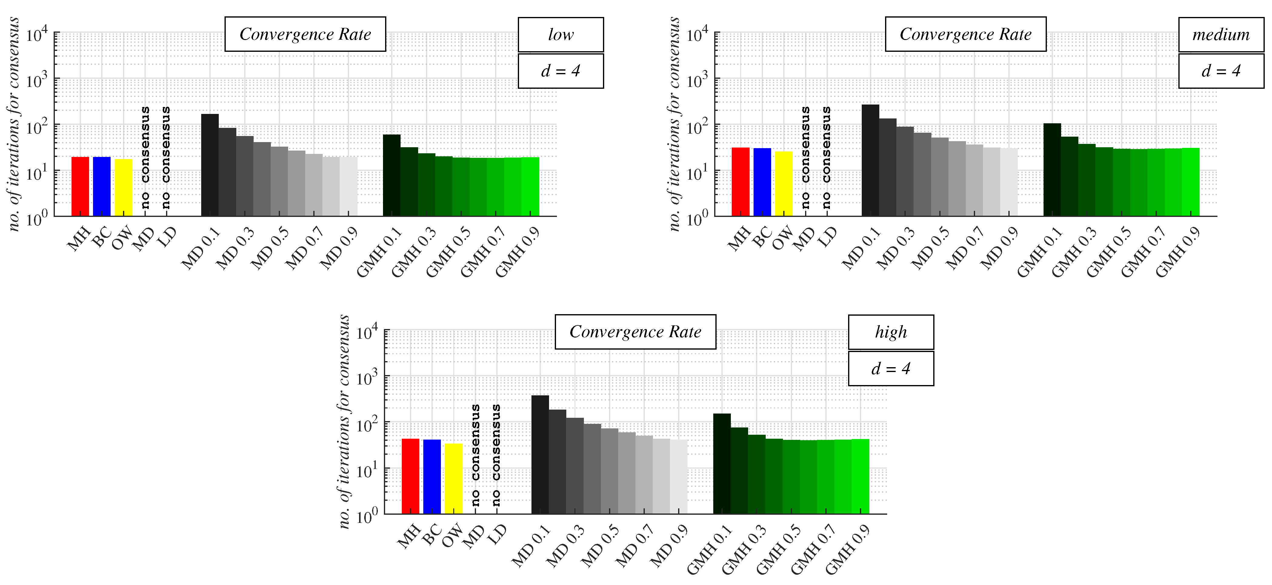
4.1. Research Methodology and Applied Metric for Performance Evaluation

This subsection is concerned with the applied research methodology and metric for performance evaluation of the analyzed distributed consensus algorithms. All the experiments were carried out in Matlab2018b (Producer: MathWorks, Location: Natick, MA, USA) using built-in Matlab functions and software designed by the authors of this paper (downloadable at [84]). As mentioned earlier in this paper, we generated random d-regular bipartite graphs with the graph order n = 30 and various degrees d. Specifically, d took the following values in our experiments:

$$d=\{2,3,4,5,10\}$$

(22)

Obviously, higher values of d result in better connectivity of generated graphs. In our experiments, we only used connected topologies since the algorithms were unable to estimate global aggregate functions in disconnected graphs (note that data can only be separately aggregated in segregated components in disconnected topologies) [52]. For every examined d, we generated 100 unique regular bipartite graphs in order to ensure the high credibility of our presented contributions (executing experiments in numerous various graphs is a common procedure in top-quality papers from the field [85,86,87]). Overall, we, thus, examined the algorithms in 500 unique graphs in this paper.

In order to evaluate the performance of the analyzed algorithms, we applied a commonplace metric used in top-quality papers in the field. Specifically, we quantified the algorithms’ performance using the convergence rate expressed as the number of iterations required for all the agents in MAS to achieve the consensus. In this case, the examined algorithms were bounded by a stopping criterion to border their execution time. In this paper, we applied the stopping criterion defined in (23), where $\mathcal{P}$ took the values from (24) [65,66].

$$\mid max\left\{\mathbf{x}\right(\mathit{k}\left)\right\}-min\left\{\mathbf{x}\right(\mathit{k}\left)\right\}\mid <\mathcal{P}$$

(23)

$$\mathcal{P}=\{{10}^{-2},{10}^{-4},{10}^{-6}\}$$

(24)

Clearly, for lower values of $\mathcal{P}$, the final estimates were assumed to be more precise but at the cost of decelerating the algorithms. Later in this paper, the precision ${10}^{-2}$ is referred to as a low precision, ${10}^{-4}$ as a medium precision, and ${10}^{-6}$ as a high precision. See Figure 8, where the maximum error of an estimate (expressed in percentages %) is depicted for each applied precision. From the figure, we can see that the low precision of the applied stopping criterion ensures that the error did not exceed 30%, the medium precision guaranteed an error lower than 0.3%, and the high precision resulted in very accurate estimates since its maximum estimation error was even lower than 0.003%.

Note that we only calculated and depicted the averaged value of the applied metric for each d and each precision of the applied stopping criterion in Section 4.2.

In order to simulate sensor-measured initial values, we generated the initial inner states of all the agents in MAS as IID (independent and identically distributed) random scalar values with the standard Gaussian distribution, i.e., [52]:

$${\mathit{x}}_{\mathit{i}}\left(0\right)\sim \mathit{N}(0,1),\phantom{.}for\phantom{.}\forall {\mathit{v}}_{\mathit{i}}\in \mathbf{V}$$

(25)

As stated above, both GMH and CW are easily modifiable algorithms since the entries of their weight matrices W contain the mixing parameter $ϵ$ [51]. In our experiments, it took the values from (26) in the case of CW and (27) if GMH was applied.

$$ϵ=\{0.1\frac{1}{\Delta },0.2\frac{1}{\Delta },0.3\frac{1}{\Delta },0.4\frac{1}{\Delta },0.5\frac{1}{\Delta },0.6\frac{1}{\Delta },0.7\frac{1}{\Delta },0.8\frac{1}{\Delta },0.9\frac{1}{\Delta }\}$$

(26)

$$ϵ=\{0.1,0.2,0.3,0.4,0.5,0.6,0.7,0.8,0.9\}$$

(27)

Later in this paper, we refer to $0.1\frac{1}{\Delta },0.2\frac{1}{\Delta },...$ from (26) as MD 0.1, MD 0.2, … etc., and 0.1, 0.2 … from (27) as GMH 0.1, GMH 0.2, …, etc.

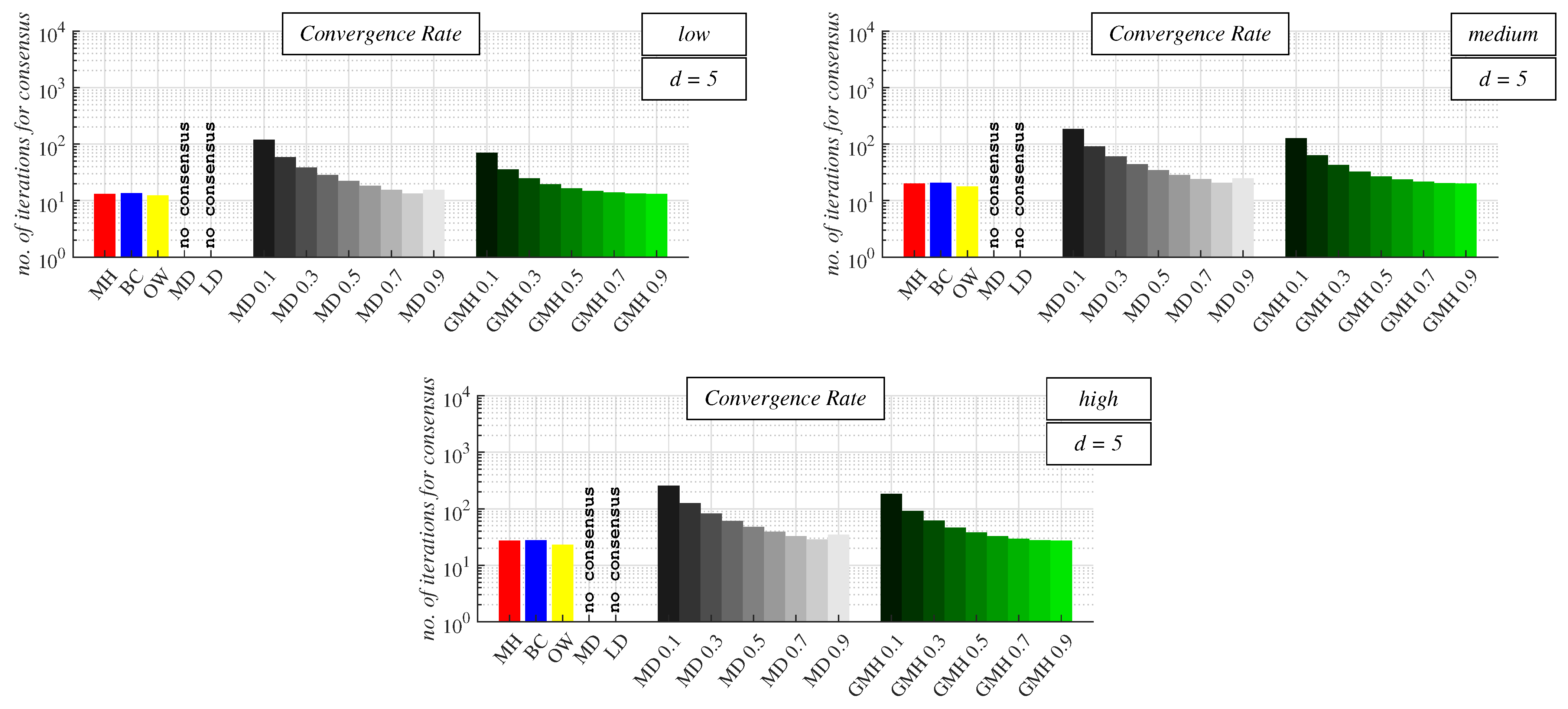
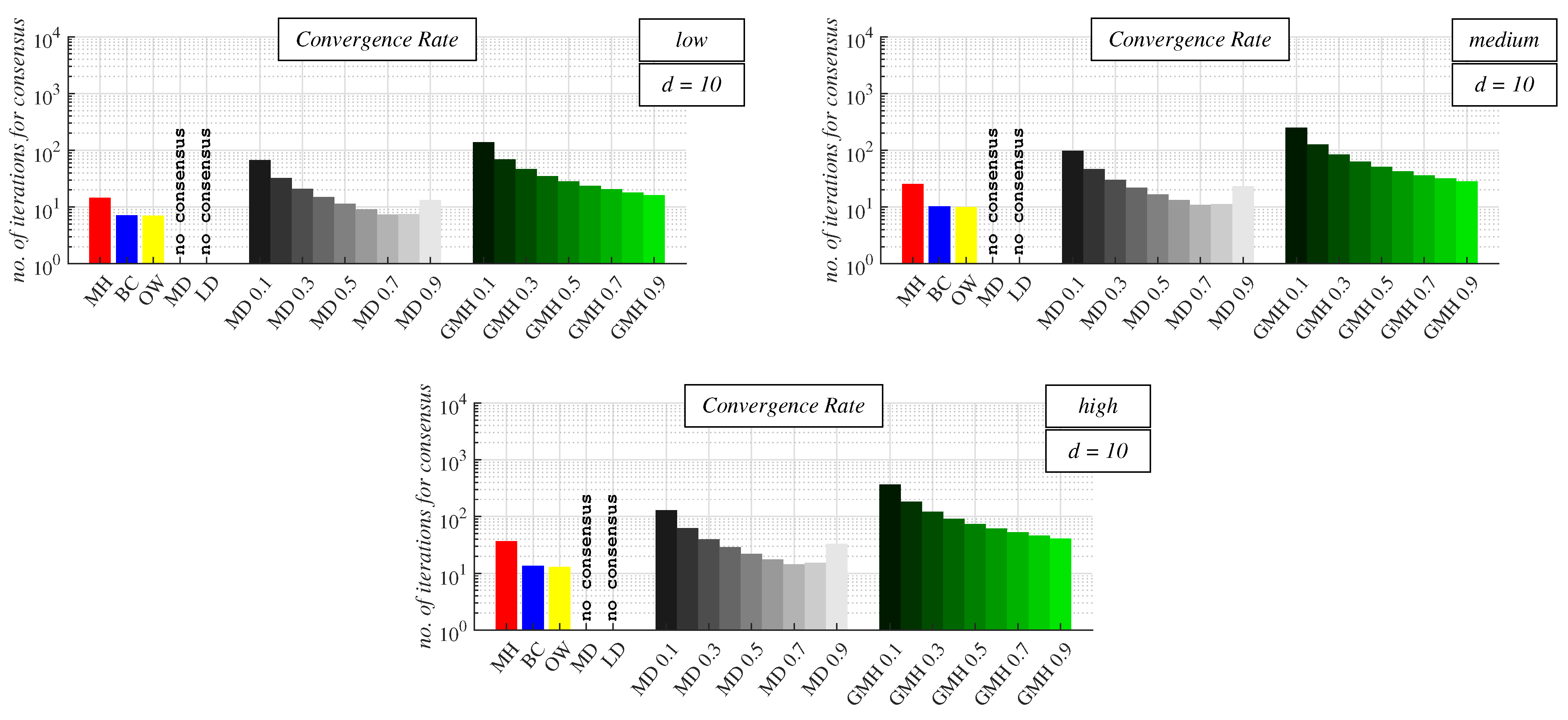
4.2. Experimental Results and Discussion about Observable Phenomena

In what follows, we focus our attention on the performance evaluation of the analyzed algorithms in regular bipartite graphs of various connectivities in order to identify whether all the algorithms can achieve the consensus and find the best-performing approach among those examined. In each connectivity graph, the algorithms were evaluated for three different precisions of the stopping criterion (the precision is provided in the right upper corner of each figure).

For d = 2 (see Figure 9 and

Table A1. Number of iterations required for consensus achievement in 2-regular bipartite graphs.

	MH	BC	OW	CW${}_{\mathit{best}}$	GMH${}_{\mathit{best}}$
Low	261.69 it.	196.75 it.	196.75 it.	193.47 it.	182.78 it.
Medium	418.54 it.	301.86 it.	301.86 it.	309.40 it.	292.16 it.
High	575.45 it.	407.27 it.	407.27 it.	425.36 it.	401.74 it.

in Appendix A) and the low precision of the applied stopping criterion, we can see that the best performance was achieved by GMH 0.1. The second-best-performing algorithm for this precision was CW, with $ϵ$ = MD 0.9. Both BC and OW achieved the same performance (as for d = 2, their matrices were identical) and were the third best among the analyzed algorithms. As further seen from the figure, the worst of the examined algorithms was MH. In the cases of the medium/high precision of the stopping criterion, GMH 0.1 outperformed all the other approaches again. Here, BC and OW were, however, better than CW and were, thus, the second best among the examined algorithms. The worst performance was observed for MH, like in the previous analysis. Moreover, it can be seen that the best performance for CW was achieved with the highest analyzed mixing parameter (i.e., $ϵ$ = MD 0.9), and its performance declined with a decrease in $ϵ$ (this is valid for each precision of the stopping criterion). For low values of $ϵ$, its performance was significantly lower than the other examined algorithms. In contrast, GMH performed the best, provided that the lowest $ϵ$ was applied (like for CW, this is valid for each precision of the stopping criterion). In addition, it can be seen from the figures that an increase in $ϵ$ resulted in performance degradation of the mentioned algorithm.

For d = 3 (see Figure 10 and

Table A2. Number of iterations required for consensus achievement in 3-regular bipartite graphs.

	MH	BC	OW	CW${}_{\mathit{best}}$	GMH${}_{\mathit{best}}$
Low	43.52 it.	39.03 it.	34.35 it.	36.31 it.	36.11 it.
Medium	70.10 it.	60.39 it.	50.88 it.	58.07 it.	57.67 it.
High	97.18 it.	81.85 it.	67.66 it.	80.48 it.	79.70 it.

in Appendix A), OW was the best-performing approach for each precision of the used stopping criterion, unlike the previous analysis. The second-best-performing algorithm, in this case, was GMH (however, with $ϵ$ = 0.3), CW with $ϵ$ = MD 0.9 was the third best, BC was the fourth one, and MH was the worst approach once again—these statements are valid for each precision of the stopping criterion for d = 3. In the case of CW, we can see that an increase in $ϵ$ resulted in better performance of the algorithm, and the highest convergence rate was obtained with $ϵ$ = MD 0.9, like for d = 2. In contrast, GMH did not achieve the highest performance with the lowest $ϵ$ (like in the previous analysis), but with $ϵ$ = 0.3. In this case, we can see that an increase in $ϵ$ ensured the algorithm accelerated until the maximum convergence rate was achieved. Afterward, a further increase in $ϵ$ resulted in the deceleration of the algorithm.

For d = 4 (see Figure 11 and

Table A3. Number of iterations required for consensus achievement in 4-regular bipartite graphs.

	MH	BC	OW	CW${}_{\mathit{best}}$	GMH${}_{\mathit{best}}$
Low	19.47 it.	19.43 it.	17.50 it.	19.31 it.	18.38 it.
Medium	31.02 it.	30.08 it.	25.44 it.	30.08 it.	28.83 it.
High	42.99 it.	40.68 it.	33.33 it.	41.16 it.	39.61 it.

in Appendix A), the best-performing algorithm for each precision of the stopping criterion was OW again. The second-best one for each precision was GMH, but now with $ϵ$ = 0.6 (note that the maximum was obtained for a greater $ϵ$ than for d = 3). Compared to the previous analysis, BC outperformed CW with the optimal mixing parameter (for d = 4, CW performed the best with $ϵ$ = MD 0.9) if the precision of the stopping criterion was medium/high. However, if its precision was low, CW performed better than BC, like in the previous analysis. MH was also the worst algorithm regarding the number of iterations required for the consensus achievement in these graphs like before. CW achieved the highest performance with the highest examined $ϵ$, like for d = 2 and 3. However, GMH achieved the maximum convergence rate with $ϵ$ = 0.6; therefore, with a higher value of the mixing parameter than for d = 3. Again, we can see that an increase in $ϵ$ resulted in a decrease in the number of iterations for consensus until the maximum convergence rate was achieved, like for d = 3. Then, a further increase in $ϵ$ caused the performance of GMH to worsen.

In addition, for d = 5 (see Figure 12 and

Table A4. Number of iterations required for consensus achievement in 5-regular bipartite graphs.

	MH	BC	OW	CW${}_{\mathit{best}}$	GMH${}_{\mathit{best}}$
Low	13.12 it.	13.54 it.	12.40 it.	13.32 it.	13.19 it.
Medium	20.07 it.	20.58 it.	17.72 it.	20.69 it.	20.10 it.
High	27.27 it.	27.79 it.	23.11 it.	28.35 it.	27.27 it.

in Appendix A), OW outperformed the concurrent algorithms for each precision of the stopping criterion, like for the two previously analyzed values of d. The second-best-performing algorithm for each precision of the used stopping criterion was paradoxically MH, which was the worst approach for d = 2, 3, and 4, as seen from Figure 9, Figure 10 and Figure 11. Thus, GMH was the best performing with $ϵ$ = 1 (i.e., MH), which is, theoretically, the slowest initial configuration in non-regular non-bipartite topologies. For the low precision, the next in order was CW, but this algorithm performed the best with $ϵ$ = MD 0.8 in this case. The worst algorithm of the applied stopping criterion for the low precision was BC: the fastest algorithm with the Perron matrix. However, for the medium/high precision of the stopping criterion, BC outperformed CW with $ϵ$ = MD 0.8. The performance of CW increased with the growth of $ϵ$ until the maximum convergence rate was obtained. A further increase in $ϵ$ caused the algorithm to decelerate. In the case of GMH, increasing $ϵ$ ensured a better performance of the algorithm.

In the largest examined graphs (i.e., d = 10, see Figure 13 and

Table A5. Number of iterations required for consensus achievement in 10-regular bipartite graphs.

	MH	BC	OW	CW${}_{\mathit{best}}$	GMH${}_{\mathit{best}}$
Low	14.56 it.	7.12 it.	7.05 it.	7.33 it.	16.11 it.
Medium	25.57 it.	10.21 it.	10.02 it.	10.82 it.	28.37 it.
High	36.86 it.	13.46 it.	13.03 it.	14.31 it.	41.03 it.

in Appendix A), OW achieved the highest performance for each precision of the applied stopping criterion again. Here, BC performed well and was the second best performing in these graphs. The third best was CW but with $ϵ$ = MD 0.7 in this case. The best-performing configuration of GMH was the configuration with $ϵ$ = 1 (MH), which was, however, outperformed by all the other concurrent approaches. As further seen from the figures, a decrease in $ϵ$ caused the performance of GMH to decline. In the case of CW, an increase in $ϵ$ ensured acceleration of the algorithm until the maximum convergence rate was achieved (note that this maximum was achieved for lower $ϵ$ than for d = 5). Afterward, a further increase in the value of $ϵ$ decelerated the algorithm, like in the previous analysis.

As also seen from Figure 9, Figure 10, Figure 11, Figure 12 and Figure 13, MD and LD algorithms diverging in regular bipartite graphs were unable to achieve the consensus for each precision of the stopping criterion. One can also observe that an increase in the precision of the stopping criterion caused all the examined algorithms to decelerate. In addition, we see that an increase in d ensured that the algorithms performed better (the only exceptions were GMH and MH).

In this paragraph, we summarize the results from Figure 9, Figure 10, Figure 11, Figure 12 and Figure 13 for each examined algorithm to identify the best-performing approach in d-regular bipartite graphs. We can see from the presented results that the performance of MH was the worst in many scenarios. Its high performance was only observed for d = 5—it was the optimal initial configuration of GMH in these graphs (and also for d = 10). However, its performance significantly degraded in the densest analyzed topologies (i.e., d = 10), and this algorithm was only better than the other configurations of GMH in these graphs. As further seen from the figures, BC performed poorly in many scenarios where the low precision of the stopping criterion was applied. As further seen, its performance can be generally considered average. However, for d = 2 (when its matrix was identical to the weight matrix W of OW) and d = 10 (i.e., in the densest examined topologies), its performance was relatively pretty good. In both these cases, its performance was the second best among the analyzed algorithms. Overall, OW was the best-performing approach according to the presented experimental results since it outperformed all the other algorithms for each precision of the used stopping criterion except for the graphs with d = 2 (the performance was lower if the low precision of the stopping criterion was applied). CW was one of the worst algorithms in terms of the number of iterations required for consensus achievement. In addition, it was necessary to know the value of d to identify the optimal configuration of this algorithm, which was its other significant drawback. However, it performed relatively well in sparsely connected graphs with the low precision of the stopping criterion. GMH outperformed all its competitors in the sparsest graphs (i.e., d = 2), but its performance was significantly degraded with an increase in connectivity (for d = 10, this was the worst algorithm among those examined). Similar to CW, knowing d was also required for the optimal configuration of this algorithm. What is most important is that all the examined algorithms except for MD and LD can achieve the consensus in each d-regular bipartite graph regardless of the precision of the applied stopping criterion. Thus, except for MD and LD, no other algorithm required the implementation of the mechanism presented in [52] or required to be reconfigured.

4.3. Comparison with Papers Concerned with Examined Algorithms in Non-Regular Non-Bipartite Graphs

In this section, we individually compare each of the examined algorithms in d-regular bipartite graphs with their performance in non-regular non-bipartite graphs analyzed in papers from Section 2.2.

MH was the worst algorithm in many examined scenarios, as seen from the figures. However, for d = 5, it was the best configuration of GMH, which does not correspond to theoretical assumptions from [51]. In these graphs, it performed well and was the second-best-performing algorithm. It was also the optimal configuration of GMH for d = 10; however, its performance was very low in this case (it even decreased compared to the performance in sparser graphs). This significant degradation of its performance in densely connected graphs was not seen in non-regular non-bipartite graphs [65,66]. In general, we can see that MH did not perform well in regular bipartite graphs, such as in non-regular non-bipartite graphs [63,65,66].

BC performed well in the densest examined graphs, which confirms the conclusions in non-regular non-bipartite graphs [66]. As identified in [63,65,66], BC usually performed poorly in sparse non-regular non-bipartite graphs, but its performance was high in 2-regular bipartite graphs (i.e., in graphs of the lowest examined connectivity). As shown in [65,66], in non-regular non-bipartite graphs, BC performed much better if the precision of the stopping criterion was not low. This statement was partially confirmed in regular bipartite graphs. In general, this algorithm achieved an average performance, which was also identified in non-regular non-bipartite graphs [62,63,65,66].

As already mentioned, OW can be considered the best-performing distributed average consensus algorithm since it outperformed the other algorithms in almost every executed scenario. The only exception was the graphs with d = 2, where this algorithm was beaten by GMH (for each precision of the applied stopping criterion) and even by CW (if the precision was low). This statement is supported by the conclusions from [64,66], where this algorithm was identified as being slow in the transient phase—the sparse connectivity of graphs caused this phase to take a longer time, and the low precision of a stopping criterion ensured that the algorithms were stopped early on. In addition, our findings in this paper correspond to the conclusions in regular bipartite graphs, where OW was mostly the best algorithm [62,63,65,66,67,68,69,70]. As shown in [63,65,66], its performance was not good in sparsely connected graphs or if the stopping criterion was operating at a low precision, like in this paper.

According to the presented results, CW was one of the worst-performing algorithms, which corresponds to its performance in non-regular non-bipartite topologies [51,62]. Its higher performance was only seen for d = 2 and the low precision of the stopping criterion. The theoretical assumption from [51] that higher values of $ϵ$ ensure better performance of the algorithm was only valid in sparser graphs. As seen from the figures, for higher values of d, the value of $ϵ$ guaranteeing its maximum performance was decreased.

Regarding GMH, this algorithm also achieved high performance, especially in sparsely connected graphs (confirmed by [64]). Similar to CW, the theoretical assumption about the optimal value of $ϵ$ was not valid again—here, a lower value of $ϵ$ did not ensure better performance in denser regular bipartite graphs in contrast to non-regular non-bipartite topologies [51]. As the graph connectivity grew, we can see that this algorithm did not achieve its maximum performance with the lowest examined value of $ϵ$. In densely connected graphs, we can see that higher connectivity caused a greater value of $ϵ$ to ensure maximum performance. Thus, our finding does not correspond to the theoretical assumptions from [51] that a lower $ϵ$ guarantees a better performing algorithm. In densely connected d-regular bipartite graphs, MH, theoretically, slowest configuration of GMH, was the optimal initial configuration of this algorithm, which does not correspond to conclusions in non-regular non-bipartite graphs [51]. As in the case of MH, the performance of this algorithm significantly decreased for d = 10—this phenomenon was not observed in non-regular non-bipartite topologies [51].

As seen in [65], all the algorithms performed better in graphs of higher connectivity. This statement is also valid in regular bipartite graphs for each algorithm except for GMH and MH, whose performance was significantly degraded in the densest examined graphs compared to graphs of sparser connectivity. Furthermore, a higher precision of the applied stopping criterion resulted in a lower convergence rate, which corresponds with the conclusions in regular bipartite graphs [65].

5. Conclusions

In this paper, we present a comparative study of seven frequently applied distributed consensus algorithms for averaging in d-regular bipartite graphs. We assumed that their execution was bounded by a stopping criterion with various precisions, whereby diverging algorithms can potentially achieve the consensus. From the presented results, it can be seen that, generally, OW was the best-performing algorithm among those examined, whereby the conclusions from non-regular non-bipartite graphs were also confirmed in this case. This algorithm did not perform the best in 2-regular bipartite graphs (i.e., in the sparsest examined graphs), where it was outperformed by GMH and CW (in this case, only for the lowest precision of the applied stopping criterion). On the other hand, MH and CW were classified as the worst-performing algorithms, which corresponds to conclusions from papers addressing these two algorithms in non-regular non-bipartite graphs. Furthermore, it was seen that each algorithm (except for GMH and MH) performed better for higher values of d (i.e., in graphs of greater connectivity). In addition, one can see that a higher precision of the applied stopping criterion caused each of the examined algorithms to decelerate. Contrary to conclusions in non-regular non-bipartite graphs, we can see that, surprisingly, GMH and CW did not achieve the optimal performance with the lowest value of $ϵ$ (in the case of GMH) and with the highest $ϵ$ (if CW was applied) in d-regular bipartite graphs of greater connectivity (this finding does not correspond to conclusions drawn in non-regular non-bipartite graphs). In this paper, all the examined algorithms were tested by investigating their convergence rate expressed as the number of iterations required for consensus achievement. The applied stopping criterion, which guaranteed the bounded execution of the algorithms, operated with three different precisions (note that the precision affects this property). Thus, in this paper, we identified that OW performed the best in d-regular bipartite graphs in terms of the number of iterations for consensus achievement, i.e., the minimum number of iterations necessary for the criterion (23) to be met for the first time. A similar/same metric is applied also in [63,65,66]. The superior performance of OW was also identified in other papers [51,62,64,67,68,69,70], where consensus algorithms are evaluated regarding various other properties, e.g., the asymptotic/per-step convergence factor, their associated convergence time, the error of the estimates, the averaging time, the mean square deviation, etc.

The final conclusion of this paper is that OW is recommended as the best-performing algorithm for d-regular bipartite graphs. Even though it was outperformed by GMH in graphs of low connectivity, we do not recommend GMH for this critical graph topology since it is not possible to identify its optimal configuration without the knowledge of d and its performance is significantly degraded in densely connected regular bipartite graphs. Moreover, it was observed that MD and LD cannot achieve consensus in spite of the application of a stopping criterion regardless of its precision—all the other analyzed algorithms operate properly in d-regular bipartite graphs for each precision of the applied stopping criterion.

References

1. Pigozzi, G.; Hartmann, S. Aggregation in multiagent systems and the problem of truth-tracking. In Proceedings of the 6th International Joint Conference on Autonomous Agents and Multiagent Systems, Honolulu, HI, USA, 14–18 May 2007; pp. 219–221. [Google Scholar]
2. Wang, J.; Yang, Y.; Wang, T.; Sherratt, R.S.; Zhang, J. Big data service architecture: A survey. J. Internet Technol. 2020, 21, 393–405. [Google Scholar]
3. Vachkova, S.N.; Petryaeva, E.Y.; Kupriyanov, R.B.; Suleymanov, R.S. School in digital age: How big data help to transform the curriculum. Information 2021, 12, 33. [Google Scholar] [CrossRef]
4. Stamatescu, G.; Chitu, C. Privacy-Preserving Sensing and Two-Stage Building Occupancy Prediction using Random Forest Learning. J. Sens. 2021, 2021, 1–12. [Google Scholar] [CrossRef]
5. Bagha, H.; Yavari, A.; Georgakopoulos, D. Hybrid Sensing Platform for IoT-Based Precision Agriculture. Future Internet 2022, 14, 233. [Google Scholar] [CrossRef]
6. Nicolae, M.; Popescu, D.; Merezeanu, D.; Ichim, L. Large scale wireless sensor networks based on fixed nodes and mobile robots in precision agriculture. Mech. Mach. Sci. 2019, 67, 236–244. [Google Scholar]
7. Abbasian Dehkordi, S.; Farajzadeh, K.; Rezazadeh, J.; Farahbakhsh, R.; Sandrasegaran, K.; Abbasian Dehkordi, M. A survey on data aggregation techniques in IoT sensor networks. Wirel. Netw. 2020, 26, 1243–1263. [Google Scholar] [CrossRef]
8. Guarino, S.; Mastrostefano, E.; Bernaschi, M.; Celestini, A.; Cianfriglia, M.; Torre, D.; Zastrow, L.R. Inferring Urban Social Networks from Publicly Available Data. Future Internet 2021, 13, 108. [Google Scholar] [CrossRef]
9. Homaei, M.H.; Salwana, E.; Shamshirband, S. An enhanced distributed data aggregation method in the Internet of Things. Sensors 2019, 19, 3173. [Google Scholar] [CrossRef]
10. Fan, H.; Liu, Y.; Zeng, Z. Decentralized privacy-preserving data aggregation scheme for smart grid based on blockchain. Sensors 2020, 20, 5282. [Google Scholar] [CrossRef]
11. Dash, L.; Pattanayak, B.K.; Mishra, S.K.; Sahoo, K.S.; Jhanjhi, N.Z.; Baz, M.; Masud, M. A Data Aggregation Approach Exploiting Spatial and Temporal Correlation among Sensor Data in Wireless Sensor Networks. Electronics 2022, 11, 989. [Google Scholar] [CrossRef]
12. Priyanka, E.B.; Thangavel, S.; Sagayam, K.M.; Elngar, A.A. Wireless network upgraded with artificial intelligence on the data aggregation towards the smart internet applications. Int. J. Syst. Assur. Eng. Manag. 2022, 13, 1254–1267. [Google Scholar] [CrossRef]
13. Ozdemir, S.; Xiao, Y. Secure data aggregation in wireless sensor networks: A comprehensive overview. Comput. Netw. 2009, 53, 2022–2037. [Google Scholar] [CrossRef]
14. Senderovich, A.; Shleyfman, A.; Weidlich, M.; Gal, A.; Mandelbaum, A. To aggregate or to eliminate? Optimal model simplification for improved process performance prediction. Inf. Syst. 2018, 78, 96–111. [Google Scholar] [CrossRef]
15. Çam, H.; Özdemir, S.; Nair, P.; Muthuavinashiappan, D.; Sanli, H.O. Energy-efficient secure pattern based data aggregation for wireless sensor networks. Comput. Commun. 2006, 29, 446–455. [Google Scholar] [CrossRef]
16. Femminella, M.; Reali, G. Gossip-based Monitoring Protocol for 6G Networks. IEEE Trans. Netw. Serv. Manag. 2023. early access. [Google Scholar] [CrossRef]
17. Ionescu, L. Digital data aggregation, analysis, and infrastructures in fintech operations. Rev. Contemp. Philos. 2020, 19, 92–98. [Google Scholar]
18. Sand, G.; Tsitouras, L.; Dimitrakopoulos, G.; Chatzigiannakis, V. A big data aggregation, analysis and exploitation integrated platform for increasing social management intelligence. In Proceedings of the 2014 IEEE International Conference on Big Data (Big Data), Washington, DC, USA, 27–30 October 2014; pp. 40–47. [Google Scholar]
19. Li, C.T.; Shih, D.H.; Wang, C.C.; Chen, C.L.; Lee, C.C. A blockchain based data aggregation and group authentication scheme for electronic medical system. IEEE Access 2020, 8, 173904–173917. [Google Scholar] [CrossRef]
20. Dhand, G.; Tyagi, S.S. Data aggregation techniques in WSN: Survey. Procedia Comput. Sci. 2016, 92, 378–384. [Google Scholar] [CrossRef]
21. Dorri, A.; Kanhere, S.S.; Jurdak, R. Multi-agent systems: A survey. IEEE Access 2018, 6, 28573–28593. [Google Scholar] [CrossRef]
22. Al-Doghman, F.; Chaczko, Z.; Jiang, J. A review of aggregation algorithms for the internet of things. In Proceedings of the 2017 25th International Conference on Systems Engineering (ICSEng), Las Vegas, NV, USA, 22–24 August 2017; pp. 480–487. [Google Scholar]
23. Izadi, D.; Abawajy, J.H.; Ghanavati, S.; Herawan, T. A data fusion method in wireless sensor networks. Sensors 2015, 15, 2964–2979. [Google Scholar] [CrossRef]
24. Stamatescu, G.; Stamatescu, I.; Popescu, D. Consensus-based data aggregation for wireless sensor networks. J. Control Eng. Appl. Inform. 2017, 19, 43–50. [Google Scholar]
25. Huang, R.; Yang, X.; Ajay, P. Consensus mechanism for software-defined blockchain in internet of things. Internet Things Cyber-Phys. Syst. 2023, 3, 52–60. [Google Scholar] [CrossRef]
26. Viriyasitavat, W.; Hoonsopon, D. Blockchain characteristics and consensus in modern business processes. J. Ind. Inf. Integr. 2019, 13, 32–39. [Google Scholar] [CrossRef]
27. Ferdous, M.S.; Chowdhury, M.J.M.; Hoque, M. A survey of consensus algorithms in public blockchain systems for crypto-currencies. J. Netw. Comput. Appl. 2021, 182, 103035. [Google Scholar] [CrossRef]
28. Claveria, O. A new consensus-based unemployment indicator. Appl. Econ. Lett. 2019, 26, 812–817. [Google Scholar] [CrossRef]
29. Ullah, M.A.; Setiawan, J.W.; ur Rehman, J.; Shin, H. On the robustness of quantum algorithms for blockchain consensus. Sensors 2022, 22, 2716. [Google Scholar] [CrossRef] [PubMed]
30. Alotaibi, R.; Alassafi, M.; Bhuiyan, M.S.I.; Raju, R.S.; Ferdous, M.S. A Reinforcement-Learning-Based Model for Resilient Load Balancing in Hyperledger Fabric. Processes 2022, 10, 2390. [Google Scholar] [CrossRef]
31. Ji, X.; Zhang, W.; Chen, S.; Luo, J.; Lu, L.; Yuan, W.; Hu, Z.; Chen, J. Speeding up velocity consensus control with small world communication topology for unmanned aerial vehicle Swarms. Electronics 2021, 10, 2547. [Google Scholar] [CrossRef]
32. Wang, C.; Mu, Z.; Mou, C.; Zheng, H.; Liu, J. Consensus-based clustering of single cells by reconstructing cell-to-cell dissimilarity. Briefings Bioinform. 2022, 23, bbab379. [Google Scholar] [CrossRef]
33. Khan, D.; Jung, L.T.; Hashmani, M.A.; Waqas, A. A critical review of blockchain consensus model. In Proceedings of the 2020 3rd international conference on computing, mathematics and engineering technologies (iCoMET), Sukkur, Pakistan, 29–30 January 2020; pp. 1–6. [Google Scholar]
34. Li, Y.; Tan, C. A survey of the consensus for multi-agent systems. Syst. Sci. Control Eng. 2019, 7, 468–482. [Google Scholar] [CrossRef]
35. Moniz, H. The Istanbul BFT consensus algorithm. arXiv 2020, arXiv:2002.03613. [Google Scholar]
36. Fan, Y.; Wu, H.; Paik, H.Y. DR-BFT: A consensus algorithm for blockchain-based multi-layer data integrity framework in dynamic edge computing system. Future Gener. Comput. Syst. 2021, 124, 33–48. [Google Scholar] [CrossRef]
37. Ma, X.; Dong, L.; Wang, Y.; Li, Y.; Sun, M. AIRC: Attentive Implicit Relation Recommendation Incorporating Content Information for Bipartite Graphs. Mathematics 2020, 8, 2132. [Google Scholar] [CrossRef]
38. Gao, W.; Aamir, M.; Iqbal, Z.; Ishaq, M.; Aslam, A. On Irregularity Measures of Some Dendrimers Structures. Mathematics 2019, 7, 271. [Google Scholar] [CrossRef]
39. Tikhomirov, K.; Youssef, P. Sharp Poincaré and log-Sobolev inequalities for the switch chain on regular bipartite graphs. Probab. Theory Relat. Fields 2023, 185, 89–184. [Google Scholar] [CrossRef]
40. Kulkarni, R. A New NC-Algorithm for Finding a Perfect Matching in d-Regular Bipartite Graphs When d Is Small. Lect. Notes Comput. Sci. 2006, 3998, 308–319. [Google Scholar]
41. Chakraborty, S.; Shaikh, S.H.; Mandal, S.B.; Ghosh, R.; Chakrabarti, A. A study and analysis of a discrete quantum walk-based hybrid clustering approach using d-regular bipartite graph and 1D lattice. Int. J. Quantum Inf. 2019, 17, 1950016. [Google Scholar] [CrossRef]
42. Arieli, I.; Sandomirskiy, F.; Smorodinsky, R. On social networks that support learning. arXiv 2020, arXiv:2011.05255. [Google Scholar] [CrossRef]
43. Zehmakan, A.N. Majority Opinion Diffusion in Social Networks: An Adversarial Approach. In Proceedings of the 35th AAAI Conference on Artificial Intelligence (AAAI 2021), Online, 2–9 February 2021; pp. 5611–5619. [Google Scholar]
44. Brandes, U.; Holm, E.; Karrenbauer, A. Cliques in regular graphs and the core-periphery problem in social networks. Lect. Notes Comput. Sci. 2016, 10043, 175–186. [Google Scholar]
45. Rödder, W.; Dellnitz, A.; Kulmann, F.; Litzinger, S.; Reucher, E. Bipartite Structures in Social Networks: Traditional versus Entropy-Driven Analyses. Entropy 2019, 21, 277. [Google Scholar] [CrossRef]
46. Galanter, N.; Silva, D., Jr.; Rowell, J.T.; Rychtář, J. Resource competition amid overlapping territories: The territorial raider model applied to multi-group interactions. J. Theor. Biol. 2017, 412, 100–106. [Google Scholar] [CrossRef]
47. El-Mesady, A.; Romanov, A.Y.; Amerikanov, A.A.; Ivannikov, A.D. On Bipartite Circulant Graph Decompositions Based on Cartesian and Tensor Products with Novel Topologies and Deadlock-Free Routing. Algorithms 2023, 16, 10. [Google Scholar] [CrossRef]
48. Pavlopoulos, G.A.; Kontou, P.I.; Pavlopoulou, A.; Bouyioukos, C.; Markou, E.; Bagos, P.G. Bipartite graphs in systems biology and medicine: A survey of methods and applications. GigaScience 2018, 7, 1–31. [Google Scholar] [CrossRef]
49. Wieling, M.; Nerbonne, J. Bipartite spectral graph partitioning for clustering dialect varieties and detecting their linguistic features. Comput. Speech Lang. 2011, 25, 700–715. [Google Scholar] [CrossRef]
50. Engbers, J.; Galvin, D. H-colouring bipartite graphs. J. Comb. Theory Ser. B 2012, 102, 726–742. [Google Scholar] [CrossRef]
51. Schwarz, V.; Hannak, G.; Matz, G. On the convergence of average consensus with generalized Metropolis-Hasting weights. In Proceedings of the 2014 IEEE International Conference on Acoustics, Speech and Signal Processing (ICASSP), Florence, Italy, 4–9 May 2014; pp. 5442–5446. [Google Scholar]
52. Kenyeres, M.; Kenyeres, J. DR-BFT: Distributed mechanism for detecting average consensus with maximum-degree weights in bipartite regular graphs. Mathematics 2021, 9, 3020. [Google Scholar] [CrossRef]
53. Kenyeres, M.; Kenyeres, J. Examination of Average Consensus with Maximum-degree Weights and Metropolis-Hastings Algorithm in Regular Bipartite Graphs. In Proceedings of the 2022 20th International Conference on Emerging eLearning Technologies and Applications (ICETA), Stary Smokovec, Slovakia, 20–21 October 2022; pp. 313–319. [Google Scholar]
54. Pandey, P.K.; Singh, R. Fast Average-consensus on Networks using Heterogeneous Diffusion. IEEE Trans. Circuits Syst. II Express Briefs 2021, 68, 1–5. [Google Scholar] [CrossRef]
55. Dhuli, S.; Atik, J.M. Analysis of Distributed Average Consensus Algorithms for Robust IoT networks. arXiv 2021, arXiv:2104.10407. [Google Scholar]
56. Kibangou, A.Y.; Commault, C. Observability in connected strongly regular graphs and distance regular graphs. IEEE Trans. Control. Netw. Syst. 2014, 1, 360–369. [Google Scholar] [CrossRef]
57. Kar, S.; Moura, J.M. Consensus based detection in sensor networks: Topology optimization under practical constraints. In Proceedings of the 1st International Workshop on Information Theory in Sensor Networks, Santa Fe, NM, USA, 18–20 June 2007; pp. 1–12. [Google Scholar]
58. Yu, J.; Yu, J.; Zhang, P.; Yang, T.; Chen, X. A unified framework design for finite-time bipartite consensus of multi-agent systems. IEEE Access 2021, 9, 48971–48979. [Google Scholar] [CrossRef]
59. Hu, J.; Zheng, W.X. Bipartite consensus for multi-agent systems on directed signed networks. In Proceedings of the IEEE Conference on Decision and Control, Firenze, Italy, 10–13 December 2013; pp. 3451–3456. [Google Scholar]
60. Han, T.; Guan, Z.-H.; Xiao, B.; Yan, H. Bipartite Average Tracking for Multi-Agent Systems with Disturbances: Finite-Time and Fixed-Time Convergence. IEEE Trans. Circuits Syst. I Regul. Pap. 2021, 68, 4393–4402. [Google Scholar] [CrossRef]
61. Muniraju, G.; Tepedelenlioglu, C.; Spanias, A. Consensus Based Distributed Spectral Radius Estimation. IEEE Signal Process. Lett. 2020, 27, 1045–1049. [Google Scholar] [CrossRef]
62. Xiao, L.; Boyd, S. Fast linear iterations for distributed averaging. Syst. Control Lett. 2004, 53, 65–78. [Google Scholar] [CrossRef]
63. Jafarizadeh, S.; Jamalipour, A. Weight optimization for distributed average consensus algorithm in symmetric, CCS & KCS star networks. arXiv 2010, arXiv:1001.4278. [Google Scholar]
64. Schwarz, V.; Matz, G. Nonlinear average consensus based on weight morphing. In Proceedings of the 2012 IEEE International Conference on Acoustics, Speech and Signal Processing (ICASSP), Kyoto, Japan, 25–30 March 2012; pp. 3129–3132. [Google Scholar]
65. Kenyeres, M.; Kenyeres, J.; Budinská, I. On performance evaluation of distributed system size estimation executed by average consensus weights. Recent Adv. Soft Comput. Cybern. 2021, 403, 15–24. [Google Scholar]
66. Kenyeres, M.; Kenyeres, J. On Comparative Study of Deterministic Linear Consensus-based Algorithms for Distributed Summing. In Proceedings of the 2019 International Conference on Applied Electronics (AE), Pilsen, Czech Republic, 10–11 September 2019; pp. 1–6. [Google Scholar]
67. Aysal, T.C.; Oreshkin, B.N.; Coates, M.J. Accelerated distributed average consensus via localized node state prediction. IEEE Trans. Signal Process. 2008, 57, 1563–1576. [Google Scholar] [CrossRef]
68. Oreshkin, B.N.; Coates, M.J.; Rabbat, M.G. Optimization and analysis of distributed averaging with short node memory. IEEE Trans. Signal Process. 2010, 58, 2850–2865. [Google Scholar] [CrossRef]
69. Schwarz, V.; Matz, G. Average consensus in wireless sensor networks: Will it blend? In Proceedings of the 2013 IEEE International Conference on Acoustics, Speech and Signal Processing, Vancouver, BC, Canada, 26–31 May 2013; pp. 4584–4588. [Google Scholar]
70. Xiao, L.; Boyd, S.; Kim, S.J. Distributed average consensus with least-mean-square deviation. J. Parallel Distrib. Comput. 2007, 67, 33–46. [Google Scholar] [CrossRef]
71. Fraser, B.; Coyle, A.; Hunjet, R.; Szabo, C. An Analytic Latency Model for a Next-Hop Data-Ferrying Swarm on Random Geometric Graphs. IEEE Access 2020, 8, 48929–48942. [Google Scholar] [CrossRef]
72. Gulzar, M.M.; Rizvi, S.T.H.; Javed, M.Y.; Munir, U.; Asif, H. Multi-agent cooperative control consensus: A comparative review. Electronics 2018, 7, 22. [Google Scholar] [CrossRef]
73. Erdös, P.; Fajtlowicz, S.; Hoffman, A.J. Maximum degree in graphs of diameter 2. Networks 1980, 10, 87–90. [Google Scholar] [CrossRef]
74. Singh, H.; Sharma, R. Role of adjacency matrix & adjacency list in graph theory. Int. J. Comput. Technol. 2012, 3, 179–183. [Google Scholar]
75. Van Nuffelen, C. On the incidence matrix of a graph. IEEE Trans. Circuits Syst. 1976, 23, 572. [Google Scholar] [CrossRef]
76. Merris, R. Laplacian matrices of graphs: A survey. Linear Algebra Its Appl. 1994, 197, 143–176. [Google Scholar] [CrossRef]
77. Mohar, B.; Alavi, Y.; Chartrand, G.; Oellermann, O.R. The Laplacian spectrum of graphs. Graph Theory Comb. Appl. 1991, 2, 12. [Google Scholar]
78. Chen, X.; Huang, L.; Ding, K.; Dey, S.; Shi, L. Privacy-preserving push-sum average consensus via state decomposition. arXiv 2020, arXiv:2009.12029. [Google Scholar] [CrossRef]
79. Merezeanu, D.; Nicolae, M. Consensus control of discrete-time multi-agent systems. U. Politeh. Buch. Ser. A 2017, 79, 167–174. [Google Scholar]
80. Yuan, H. A bound on the spectral radius of graphs. Linear Algebra Its Appl. 1988, 108, 135–139. [Google Scholar] [CrossRef]
81. Xiao, L.; Boyd, S.; Lall, S. A scheme for robust distributed sensor fusion based on average consensus. In Proceedings of the Fourth International Symposium on Information Processing in Sensor Networks, Boise, ID, USA, 15 April 2005; pp. 63–70. [Google Scholar]
82. Strand, M. Strand, M. Metropolis-Hastings Markov Chain Monte Carlo; Chapman University: Orange, CA, USA, 2009. [Google Scholar]
83. Avrachenkov, K.; El Chamie, M.; Neglia, G. A local average consensus algorithm for wireless sensor networks. In Proceedings of the 2011 International Conference on Distributed Computing in Sensor Systems and Workshops (DCOSS), Barcelona, Spain, 27–29 June 2011; pp. 1–6. [Google Scholar]
84. Codes for the Paper “Distributed Average Consensus Algorithms in d-Regular Bipartite Graphs: Comparative Study”. Available online: https://github.com/kenyeresm/regularbipartite (accessed on 11 May 2023).
85. Pereira, S.S.; Pagès-Zamora, A. Mean square convergence of consensus algorithms in random WSNs. IEEE Trans. Signal Process. 2010, 58, 2866–2874. [Google Scholar] [CrossRef]
86. Skorpil, V.; Stastny, J. Back-propagation and k-means algorithms comparison. In Proceedings of the 2006 8th International Conference on Signal Processing (ICSP 2006), Guilin, China, 16–20 November 2006; pp. 374–378. [Google Scholar]
87. Lee, C.S.; Michelusi, N.; Scutari, G. Finite rate distributed weight-balancing and average consensus over digraphs. IEEE Trans. Autom. Control 2020, 66, 4530–4545. [Google Scholar] [CrossRef]
Figure 1. Characteristic features of agents forming multi-agent systems.
Futureinternet 15 00183 g001
Figure 2. Process of data aggregation in examined scenario.
Futureinternet 15 00183 g002
Figure 3. Group of eight children with and without consensus.
Futureinternet 15 00183 g003
Figure 4. Network with three broken conditions required to be met by consensus algorithms and error-free execution—min-consensus is applied.
Futureinternet 15 00183 g004
Figure 5. Example of 3-regular bipartite graphs formed by fourteen vertices.
Futureinternet 15 00183 g005
Figure 6. Comparison of evolution of inner state in regular bipartite/non-regular non-bipartite graph.
Futureinternet 15 00183 g006
Figure 7. Example of spectrum of weight matrix W of each examined algorithm.
Futureinternet 15 00183 g007aFutureinternet 15 00183 g007b
Figure 8. Maximum error of used precisions of applied stopping criterion.
Futureinternet 15 00183 g008
Figure 9. Convergence rate expressed as number of iterations required for consensus achievement in 2-regular bipartite graphs and for three precisions of applied stopping criterion.
Futureinternet 15 00183 g009
Figure 10. Convergence rate expressed as number of iterations required for consensus achievement in 3-regular bipartite graphs and for three precisions of applied stopping criterion.
Futureinternet 15 00183 g010
Figure 11. Convergence rate expressed as number of iterations required for consensus achievement in 4-regular bipartite graphs and for three precisions of applied stopping criterion.
Futureinternet 15 00183 g011
Figure 12. Convergence rate expressed as number of iterations required for consensus achievement in 5-regular bipartite graphs and for three precisions of applied stopping criterion.
Futureinternet 15 00183 g012
Figure 13. Convergence rate expressed as number of iterations required for consensus achievement in 10-regular bipartite graphs and for three precisions of applied stopping criterion.
Futureinternet 15 00183 g013
Disclaimer/Publisher’s Note: The statements, opinions and data contained in all publications are solely those of the individual author(s) and contributor(s) and not of MDPI and/or the editor(s). MDPI and/or the editor(s) disclaim responsibility for any injury to people or property resulting from any ideas, methods, instructions or products referred to in the content.