Article

A Comparative Study of Single and Multi-Stage Forecasting Algorithms for the Prediction of Electricity Consumption Using a UK-National Health Service (NHS) Hospital Dataset

1
James Watt School of Engineering, College of Science and Engineering, University of Glasgow, Glasgow G12 8QQ, UK
2
School of Computer Science, University of Sunderland, Sunderland SR6 0DD, UK
3
Independent Researcher, Dover, NH 03820, USA
4
Brunel Interdisciplinary Power Systems Research Centre, Brunel University London, London UB8 3PH, UK
*
Authors to whom correspondence should be addressed.
These authors contributed equally to this work.
Future Internet 2023, 15(4), 134; https://doi.org/10.3390/fi15040134
Submission received: 10 February 2023 / Revised: 25 March 2023 / Accepted: 27 March 2023 / Published: 31 March 2023
(This article belongs to the Special Issue Smart Objects and Technologies for Social Good II)

Abstract

:
Accurately looking into the future was a significantly major challenge prior to the era of big data, but with rapid advancements in the Internet of Things (IoT), Artificial Intelligence (AI), and the data availability around us, this has become relatively easier. Nevertheless, in order to ensure high-accuracy forecasting, it is crucial to consider suitable algorithms and the impact of the extracted features. This paper presents a framework to evaluate a total of nine forecasting algorithms categorised into single and multistage models, constructed from the Prophet, Support Vector Regression (SVR), Long Short-Term Memory (LSTM), and the Least Absolute Shrinkage and Selection Operator (LASSO) approaches, applied to an electricity demand dataset from an NHS hospital. The aim is to see such techniques widely used in accurately predicting energy consumption, limiting the negative impacts of future waste on energy, and making a contribution towards the 2050 net zero carbon target. The proposed method accounts for patterns in demand and temperature to accurately forecast consumption. The Coefficient of Determination ( R 2 ), Mean Absolute Error (MAE), and Root Mean Square Error (RMSE) were used to evaluate the algorithms’ performance. The results show the superiority of the Long Short-Term Memory (LSTM) model and the multistage Facebook Prophet model, with R 2 values of 87.20 % and 68.06 % , respectively.

1. Introduction

Recently, the National Health Service (NHS) of the United Kingdom (UK) outlined plans to achieve net zero emissions by 2050, with an 80 % reduction by 2028–2032 [1]. The NHS generates 18 % of all emissions deriving from the UK’s non-domestic buildings [2]. This is mainly due to the high energy consumption of hospitals. For the sake of reducing energy consumption, hospitals can adopt precise forecasting techniques to predict energy usage and facilitate the development of effective solutions to overcome potential increases.
In this context, multiple forecasting techniques have been proposed in recent years, and they can be categorised into, but not limited to, time series models, regression models, econometric models, genetic algorithm models, and others [3]. Time series models are simple, as they use the time-series trends from time-stamped historical data to predict the future energy demand. This work implements and utilises time series models that predict future energy consumption based on previously captured time-stamped data.
Load forecasting of electricity demand has been widely investigated, with studies considering various sectors and geographical locations, and it is categorised into short-, medium-, and long-term forecasting. Short-term forecasting has been considered by [4,5,6,7] and can typically predict from an hour to a week into the future. Medium-term forecasting, on the other hand, can range between a week and a year; an example is the studies conducted by [8], in which the authors used 5 years of data to predict the 6th year. Finally, long-term forecasting can predict up to 5 years into the future [9]. In this paper, we implement time series models to perform medium-term electricity demand forecasting, primarily using Facebook’s Prophet (FBP), Support Vector Regression (SVR), and Long Short-Term Memory (LSTM), all of which are commonly used algorithms for forecasting time series data.
FBP is an open-source modular regression algorithm developed and released by Facebook’s Core Data Science team [10]. As a time series forecasting algorithm, it excels when dealing with data/time series that have strong seasonal effects. The LSTM algorithm is considered one of the most effective Recurrent Neural Network (RNN)-based architectures. It is mainly used in, and excels in, natural language processing and forecasting time series, due to its capability of saving statistical values from earlier stages to be used in predicting future estimates [11,12,13]. The SVR algorithm is adapted from the Support Vector Machine (SVM). It is a regression algorithm that is developed to robustly and flexibly model nonlinear relationships between variables. This enables better interpretation of the resulting models. Because SVR works on nonlinear models, it uses kernels to transform the data into a linear equation with a high number of dimensions [14,15].
In the current state of the art, researchers have employed numerous techniques to perform electricity demand forecasting. The authors in [16] discuss the importance of electric load forecasting in maintaining the balance between electric power generation and consumption, and its role in ensuring the reliability and stability of the power grid. The article describes various methods of load forecasting, including linear regression, econometric models, fuzzy models, data mining procedures, and AutoRegressive Integrated Moving Average (ARIMA) models, and highlights the use of artificial neural networks in load forecasting. The article also proposes a load forecasting model based on a neural network and a wavelet denoising algorithm, and presents real recorded data from the Bulgarian power system grid to demonstrate the effectiveness of the proposed method in reducing the relative error between real and theoretical data.
In [17], the authors explore the use of Artificial Neural Network (ANN) models to predict future energy consumption. Various ANN models with different structures, learning algorithms, and transfer functions were created and tested using actual input and output data for training, validation, and testing. The goal was to identify the best model with the greatest generalisation ability. The chosen ANN model was then used to predict energy consumption in Greece in the coming years. The Feed-Forward (FF) ANN method was used, and several models were developed and compared to select the most suitable one. The MATLAB neural network toolbox was used to train the models, with input and output data from the previous 15 years used for training and validation. The Levenberg-Marquardt and Gradient Descent learning algorithms and hyperbolic tangent sigmoid, logarithmic sigmoid, and hard-limit transfer functions were used, with structures consisting of 1 to 5 hidden layers with 2 to 40 neurons in each hidden layer. The selected model was the Levenberg-Marquardt-Logarithmic Sigmoid (with a structure: 4/12/11/1), as it had the best generalising ability, a compact structure, a fast training process, and low memory consumption. ANN models were found to be effective in predicting energy consumption thanks to their computational speed, ability to handle complex nonlinear functions, and robustness even when full information is not available.
Some authors went on to explore the impact of hybrid models on the overall performance of the forecasting process. For instance, the authors in [18] investigated the use of a hybrid approach by combining Singular Spectrum Analysis (SSA) and ANNs for day-ahead hourly load forecasting. The extracted components are employed as exogenous regressors in a global forecasting model, comprising either a Multilayer Perceptron (MLP) or an LSTM predictive layer. The model is further extended to include exogenous features, such as weather forecasts. The predictive performance is evaluated on two real-world datasets, and the results show that the decomposition step improves the relative performance of ANN models, with a combination of LSTM and SSA providing the best overall performance.
Furthermore, Aravazhi et al. [19] proposed a model that predicts load demand for different hospital usage scenarios by using a dual hybrid combination of four simple models: Seasonal-ARIMA (SARIMA), SVR, MLP, and LSTM. Experimental results show that there are corresponding matching models for unique usage scenarios. For example, in one case, a single LSTM model performed better in predicting the demand for inpatient day shift surgery in a Norwegian hospital, while a hybrid model performed more effectively in most cases.
Bagnasco et al. [20] proposed the use of multilayer perception BP neural networks as a forecasting algorithm to predict electricity consumption in Cellini medical clinic in Turin, using time series data of load data, day type, and weather data as input features, and Mean Absolute Percentage Error (MAPE), Daily Peak MAPE, Coefficient of the Variation of the Root Mean Square Error (CVRMSE), Mean Percentage Error (MPE), and MAPE under 5% as forecasting assessment metrics. In [21], the authors conducted a study to see which has a higher impact on the forecasting accuracy, the neural network or the learning algorithm. In their paper, the performance of MLP and Elman neural networks in electric load forecasting was compared. Using a dataset from a power utility in Thessaloniki, Greece, the authors performed short-term forecasting to predict one week ahead in order to test the network’s generalisation ability. Different combinations of prediction order and the number of neurons in the hidden layer were used to find the architecture that would model the data most effectively. The MATLAB Neural Networks toolbox was used to initialise, train, and test both the MLP and Elman networks. The Mean Square Error (MSE) was used to measure network performance, and the results show that the efficiency of the learning algorithm is more important than the neural network model used for forecasting. The authors found that the Elman network models the considered electric load series better than the MLP network, but training the Elman network is two to five times slower than training the MLP network. The time required for training depends on the training data size and the number of network parameters. However, the learning algorithms used with the Elman network were not able to fully implement the richer structure of this network. A synthesis that includes the advantages and disadvantages of the techniques and algorithms proposed in the literature are presented in Table 1 and Table 2.
In this paper, we perform a comparative study that includes a total of nine forecasting algorithms to investigate the impact of hybrid models and the incorporation of weather data on the overall accuracy of forecasting electricity demand in an NHS hospital. The strengths and main contributions of the study are summarised as follows:
  • The use of a comparative study design and the inclusion of multiple forecasting algorithms allow for a robust analysis of the proposed technique.
  • The impact of hybrid models and weather data on electricity demand forecasting is assessed.
  • The use of an NHS hospital as the case study provides a relevant and practical application of the research, which could have important implications for hospital energy management and efficiency.
The paper is structured as follows. Section 2 outlines the data used, Section 3 describes the methodology, Section 4 presents our obtained results, and finally, Section 5 concludes the paper and suggests potential future directions.

2. Data

This section outlines the details of the data used in this study. The first dataset contains data related to electricity demand, which is the main focus of this study. The dataset was collected as part of a previous study [22] conducted in an NHS hospital (Medway NHS Foundation Trust) located in the south-east of England. The second dataset constitutes measurements of the average temperature. The following subsections, Section 2.1 and Section 2.2, highlight more details about the electricity demand and weather datasets, respectively, including, where applicable, details of data collection.

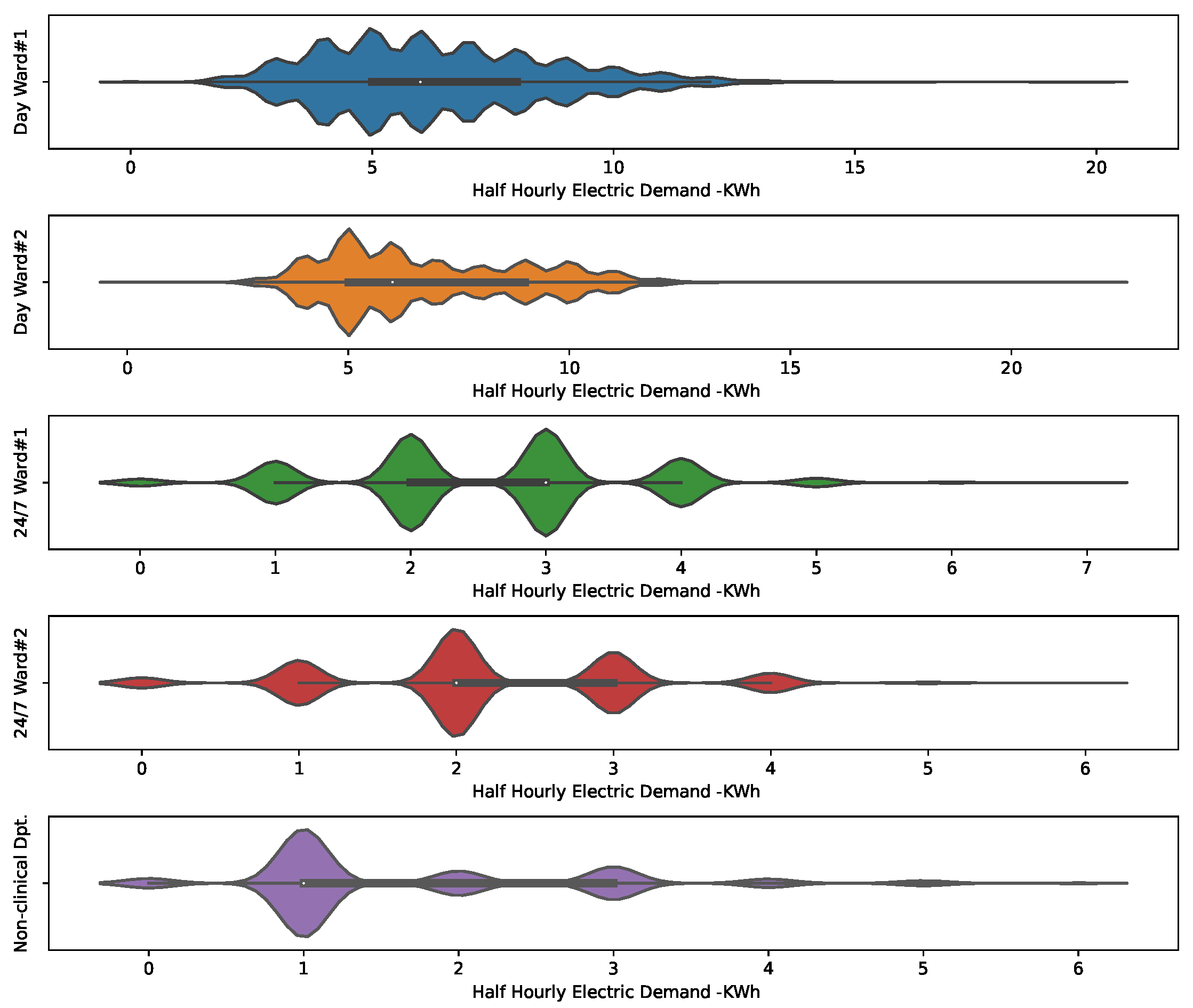
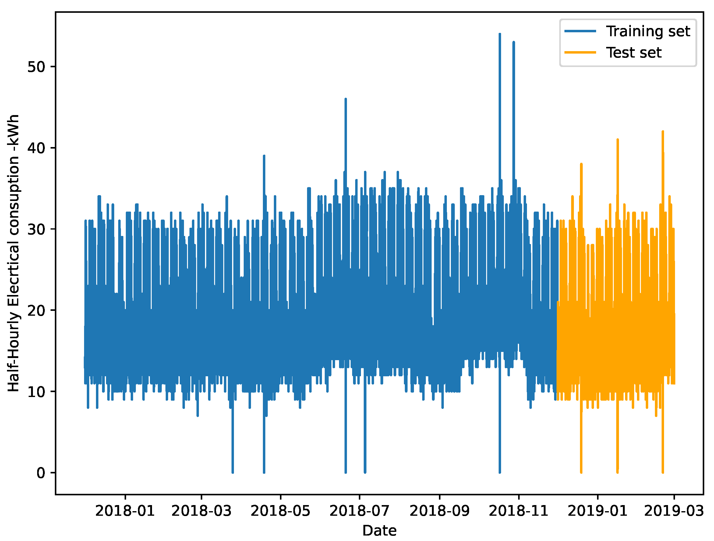
2.1. NHS Electricity Demand Dataset

The dataset reflects the Half-Hourly (HH) electricity consumption of a diverse group of wards/departments in the hospital, including four clinical areas (two of which operate 24 / 7 , while the other two operate only during the day) and one non-clinical. The data were collected using a Wireless Electricity Data Logger (WEDL) system provided by EnergyLogix [23] (see [22] for more details about the system), which obtained consumption data directly from the hospital’s electricity meters. The data used in this study covered a period of 15 months, from December 2017 to the end of February 2019. The electricity meters pulsed 1 kWh pulses, which were collected for half an hour by the WEDL and pushed to the server every hour. Figure 1 shows a violin plot visualising the descriptive statistics of the dataset used.
Note that the data were collected for each ward/department separately during the data collection phase. In this study, the dataset is combined and treated as one to provide a comprehensive representation of an entire hospital unit.

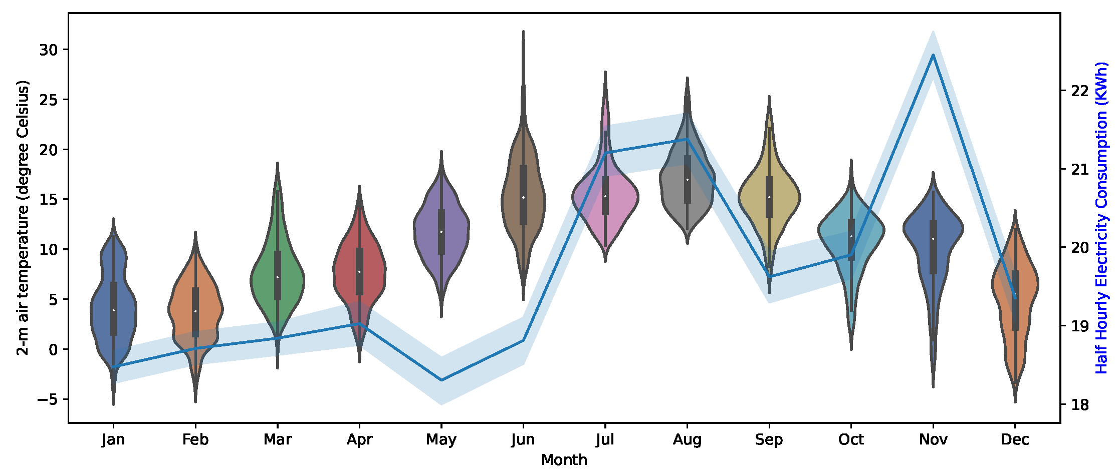
2.2. Weather Dataset

The weather dataset is obtained from the European Commission’s science and knowledge service, EU Science Hub [24]. The dataset consists of hourly recordings of the Typical Meteorological Year (TMY) 2-m air temperature in the hospital location for the period of 2007–2016. The TMY is obtained as shown in Table 3. The mean TMY temperature is 10.36, and the standard deviation is 5.57. Figure 2 shows the box plot of the temperature and the half-hourly electricity consumption. As mentioned earlier, and among other things, this study sets out to investigate the impact of an external factor, such as the temperature, on the overall forecasting results.

3. Forecasting Models and Evaluation Metrics

This section aims to present the core methodology adopted in conducting this study by outlining the developed forecasting models and their testing and evaluation performed in this study. The testing, which applies to all models and methods adopted in this paper, was performed by splitting the electricity demand dataset into 12 months for training (from 1 December 2017 to 1 December 2018) and 3 months for testing (from 1 December 2018 to 28 February 2019), using the train-test split method (see Figure 3).

3.1. Forecasting Models

As mentioned before, in this work, we focused on using quantitative models because we relied on previous data to predict future ones. We focused on three algorithms, namely FBP, LSTM, and SVR, and compared them to the LASSO algorithm which captures the linear relationship between the data [25].
In our experiments, we set up these algorithms as follows.
  • FBP: The yearly, weekly, and daily seasonality are all set to increase forecasting accuracy and reliability.
  • LSTM: The architecture used consists of one input, one hidden, and one output layer, with one, two hundred, and one nodes, respectively.
  • SVR: The “RBF” kernel is used, due to its ability to deal with the high space complexity problem.

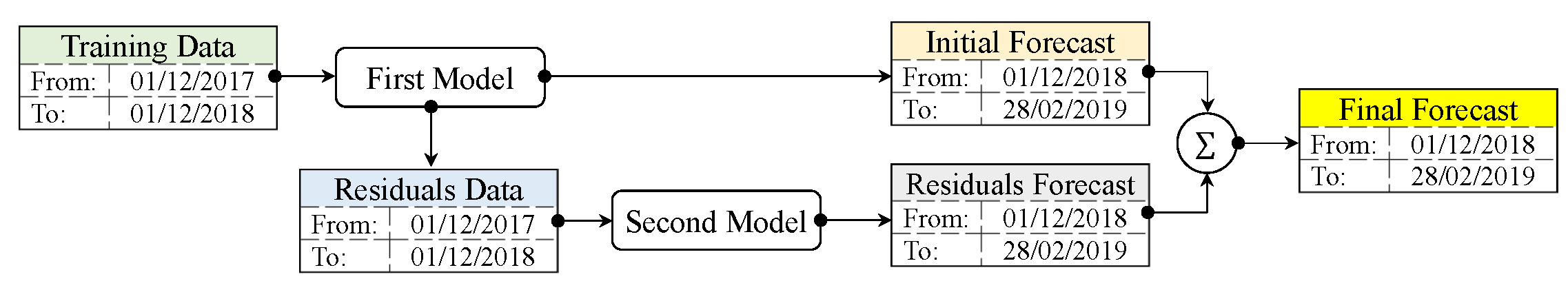
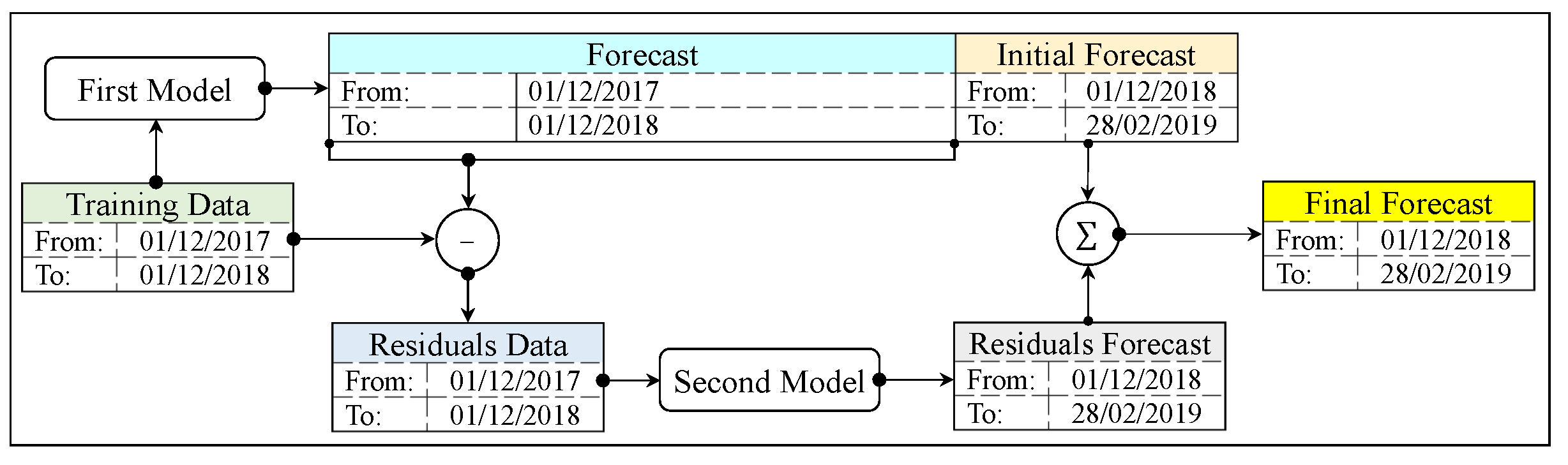
3.1.1. Multistage Forecasting

In this study, a multistage model is designed, consisting of two stages and constructed from a different combination of forecasting algorithms, to examine the impact this might have on the accuracy of the forecasting. Let us assume that the initial forecast is denoted by y ^ 1 ( t ) for time t ϵ { 0 T R } , where T R is the last data point of the training set. The residuals, denoted by e ( t ) , are the differences between the actual values and the initial forecast.
e ( t ) = y ( t ) y ^ 1 ( t )
We can then use these residuals to forecast the future residuals, which we will call e ^ ( t ) . The hybrid forecasting model that incorporates these two forecasts can be represented mathematically as:
y ^ ( τ ) = y ^ 1 ( τ ) + e ^ ( τ )
where y ^ ( τ ) is the final forecast at time τ ϵ { T R T S } , T S refers to the last data point of the test set.
In other words, this model combines the information from the initial forecast with the information contained in the historical residuals to generate a more accurate final forecast. Figure 4 visualises the multistage modeling process.
Figure 5 further expands on Figure 4 to describe the multistage forecasting process. In the first stage of the multistage model, the training data acts as input to the “First Model”. Part of the output from the “First Model” is used to compute the “Residuals Data”, and the other part becomes the “Initial Forecast”. The “Residuals Data” is then passed on to the “Second Model” to obtain the “Residuals Forecast”, which is then arithmetically added to the “Initial Forecast” to give the “Final Forecast” data.
For this paper, the multistage model is implemented using two different approaches. The first involves having the same algorithm in both stages of the model; that is, the “First Model” and “Second Model” are the same (see Figure 4). In the second approach, a hybrid of models is used; that is, the “First Model” and “Second Model” are different, such as SVR-LSTM. The following are the multistage models utilised in this study:
  • Multistage models with similar algorithms
    • SVR-SVR
    • FBP-FBP
  • Multistage models with hybrid algorithms
    • FBP-SVR
    • FBP-LSTM
    • SVR-LSTM

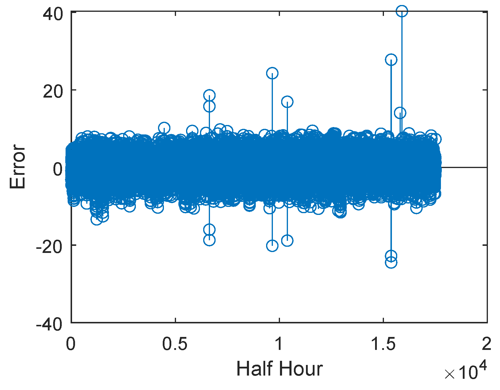
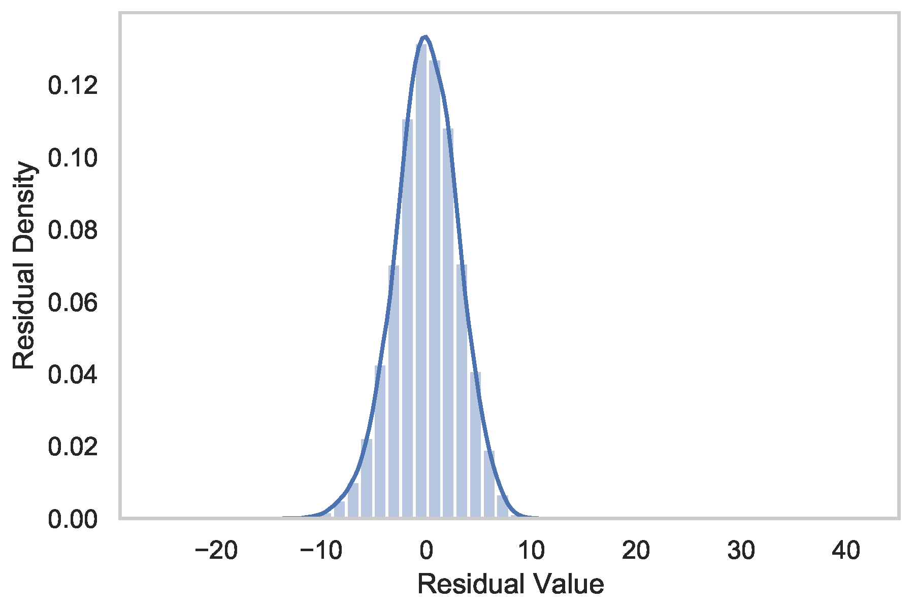
3.1.2. Limitations of Residual Forecasting

The residual forecasting method is a statistical technique that involves fitting a model to historical data and then using the residuals, which are the differences between the actual values and the predicted values, to forecast future values. The residual forecasting method can be a useful tool for forecasting time series data, particularly when the data contain complex patterns that are difficult to model using traditional methods. However, it also has some limitations. Outlined below are some advantages and limitations of using the residual forecasting method.
  • Advantages
    Simplicity: The method is easy to implement and requires minimal technical expertise.
    Flexibility: The method can be applied to a wide range of forecasting problems, including time series forecasting and regression analysis.
    Improved accuracy: By accounting for the residual errors in the forecasting model, the residual forecasting method can lead to more accurate predictions.
    Transparency: The method is transparent and provides insight into the forecasting process, which can help decision-makers understand the sources of uncertainty in the forecasts.
  • Limitations
    Limited by time horizon: Residual forecasting is most effective in predicting outcomes over short to medium time horizons. Over longer time horizons, the accuracy of the predictions may decrease, particularly if there are significant changes in external factors that were not accounted for in the historical data.
    Dependence on underlying model: The accuracy of the forecasts is heavily dependent on the accuracy of the underlying model used to estimate the residuals.
    Assumption of stationarity: The method assumes that the residual errors are stationary over time, which may not always be the case.
    Ignoring other sources of uncertainty: The method only accounts for residual errors and ignores other sources of uncertainty, such as measurement errors or random fluctuations.

3.2. Metrics to Evaluate the Forecasting Models

In this work, three kinds of error metrics are examined for the hybrid forecasting models, as follows:
  • The coefficient of determination ( R 2 ):
    R 2 = 1 R S S T S S
    where R S S is the sum of squares of residuals, and T S S is the total sum of squares.
  • Mean Absolute Error (MAE):
    M A E = 1 n j = 1 n | y j y ^ j |
  • Root Mean Square Error (RMSE):
    R M S E = 1 n j = 1 n ( y j y ^ j ) 2
    where n is the number of samples, and y and y ^ are the predicted value and actual value, respectively.
A key feature of the error metrics employed for model evaluations is their ability to differentiate among model results. The metric that identifies higher variations in regression models’ performance is often the more desirable. In this instance, MAE could be impacted by many average error values without sufficiently showing some of these large errors. The RMSE could be better at identifying model performance differences by providing higher weighting to unfavorable conditions.
It is well known that the sensitivity of the RMSE to outliers is one of the key concerns when using this metric. In practical situations, it is common for modelers to omit the outliers that are several orders greater than the other samples when computing the RMSE, especially if the sample size is small. If the model biases are significant, the systematic errors may need to be removed before computing the RMSEs.
One key merit of RMSEs over MAEs is that RMSEs do not need to compute the absolute value, which is highly undesirable in many mathematical calculations. For example, it may be challenging to compute the sensitivity or gradient of the MAEs with respect to model parameters. In addition, in data assimilation, the sum of squared errors is usually defined as the cost function to be minimised by adjusting model parameters [26]. In this case, penalising large errors through the defined least-square terms is demonstrated to be effective in enhancing model performance. In the scenarios of computing model error sensitivities or data as simulation applications, MAEs are not favored over RMSEs.

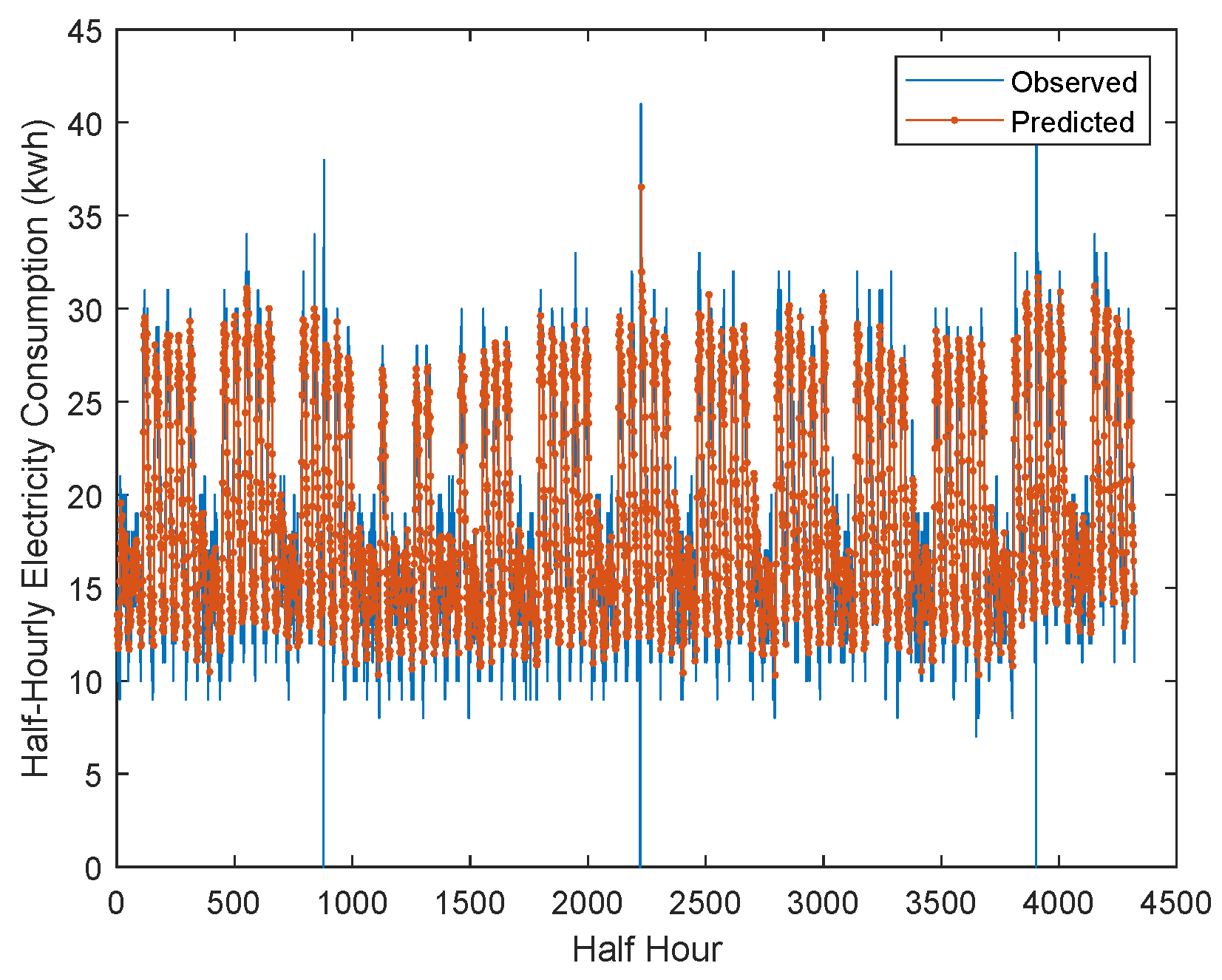
4. Forecasting Results and Discussion
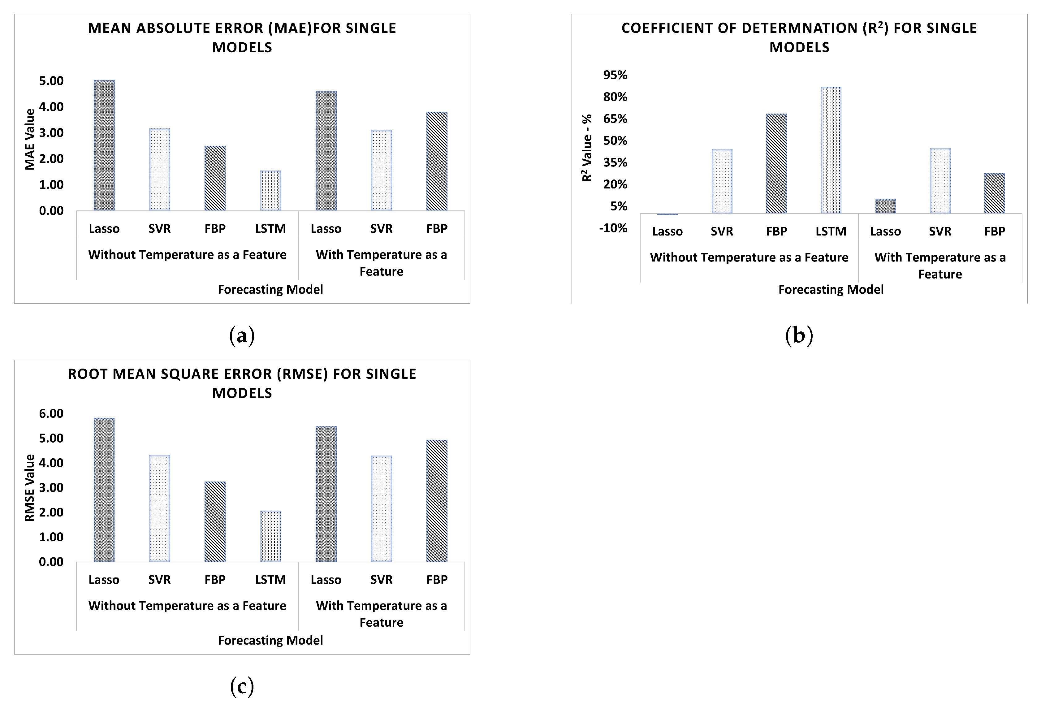
This section aims to present the results obtained from forecasting the electricity demand data, as previously outlined in Section 3.1. The implemented approach is to evaluate the performance of single and multistage models to see which is best to be used to accurately forecast the data. This section therefore opens with Section 4.1, which will show the results of the single models, that is, the LASSO, FBP, LSTM, and SVR. Section 4.2 will then highlight the results obtained from running the multistage models with similar algorithms, that is, SVR-SVR and FBP-FBP, and Section 4.3 will present the results obtained from the multistage models with hybrid algorithms, that is, FBP-SVR, FBP-FBP, FBP-LSTM, and SVR-LSTM. Finally, Section 4.4 will present the results of the comparative study by comparing the computed metrics, that is, R 2 , MAE, and RMSE, of all the single and multistage models. The forecasting for each single/multistage model is performed in the presence and absence of the temperature data as a predicting feature, details of which were presented earlier in Section 2.2.

4.1. Single Models

Four single models were developed to be tested using the electricity demand dataset. The outputs from these models are computed, and their performances are compared using the three metrics R 2 , MAE, and RMSE, as highlighted earlier in Section 3.2. Table 4 shows a comparison which is further visualised in Figure 6. The performance evaluation is performed on the models after training them on the electricity demand dataset with and without the use of the temperature as a training feature.
As seen in Table 4 and Figure 6, the LSTM outperforms all other models with an R 2 of 87.20 % , an MAE of 1.55 , and an RMSE of 2.08 . Figure 7 shows the predicted/forecasted output against the testing data, which span the period between 1 December 2018 and 28 February 2019, as shown earlier in Figure 3. The figure visualises a close similarity between both datasets with minor differences. It is also worth mentioning that the addition of the temperature as a feature did not improve the results. There is a negligible improvement with the LASSO and SVR models, and a decrease in performance for the FBP. This indicates that the energy consumption is not impacted by the changes in temperature, and this can also be visually seen in Figure 2.

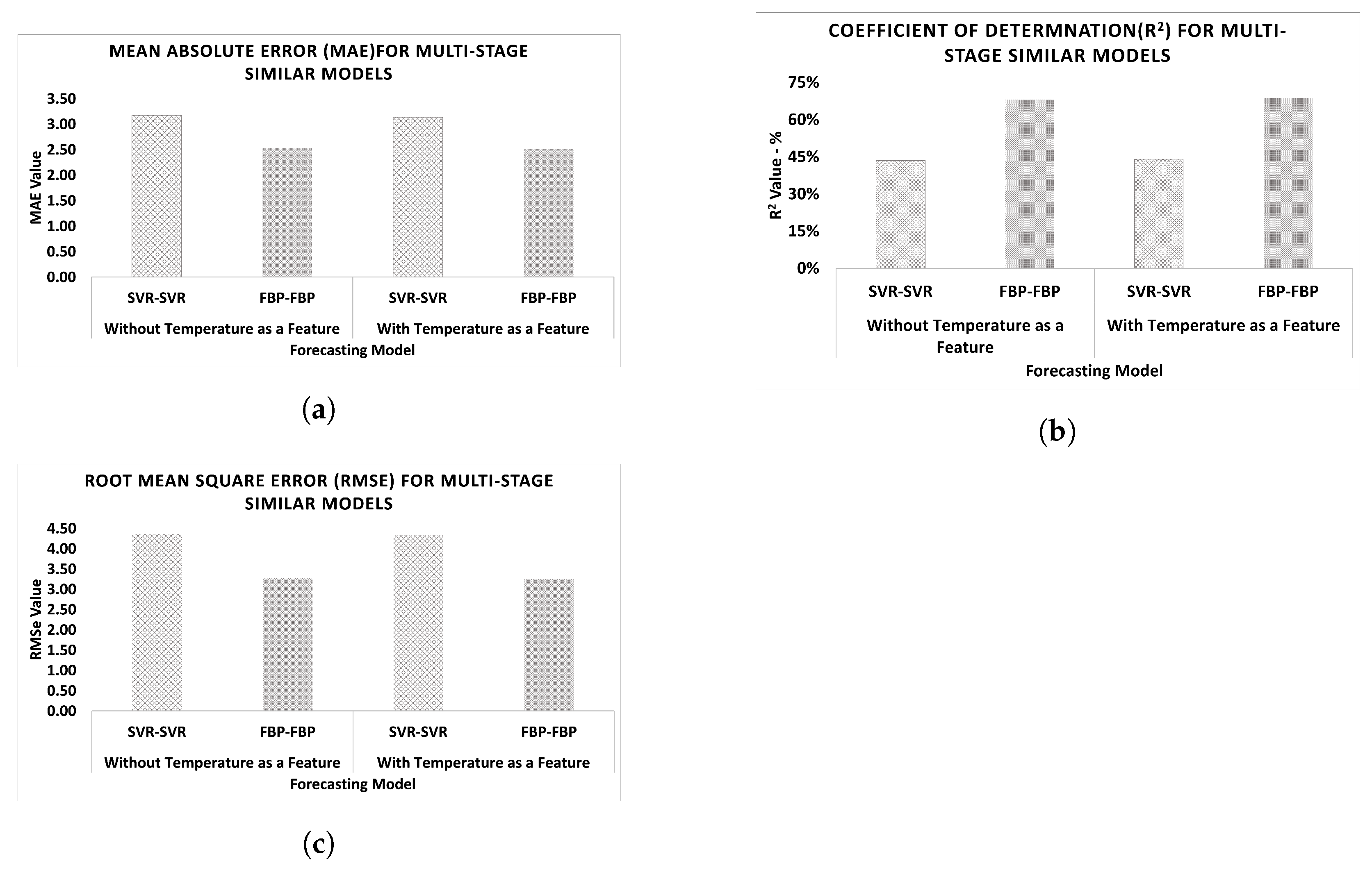
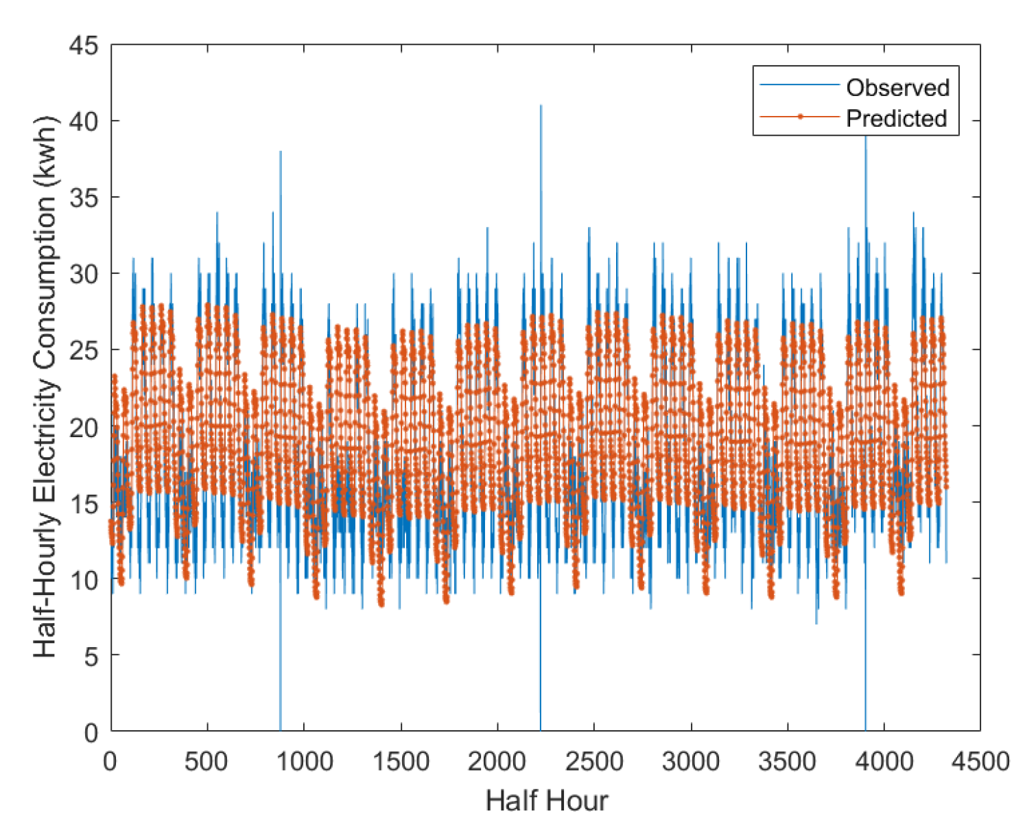
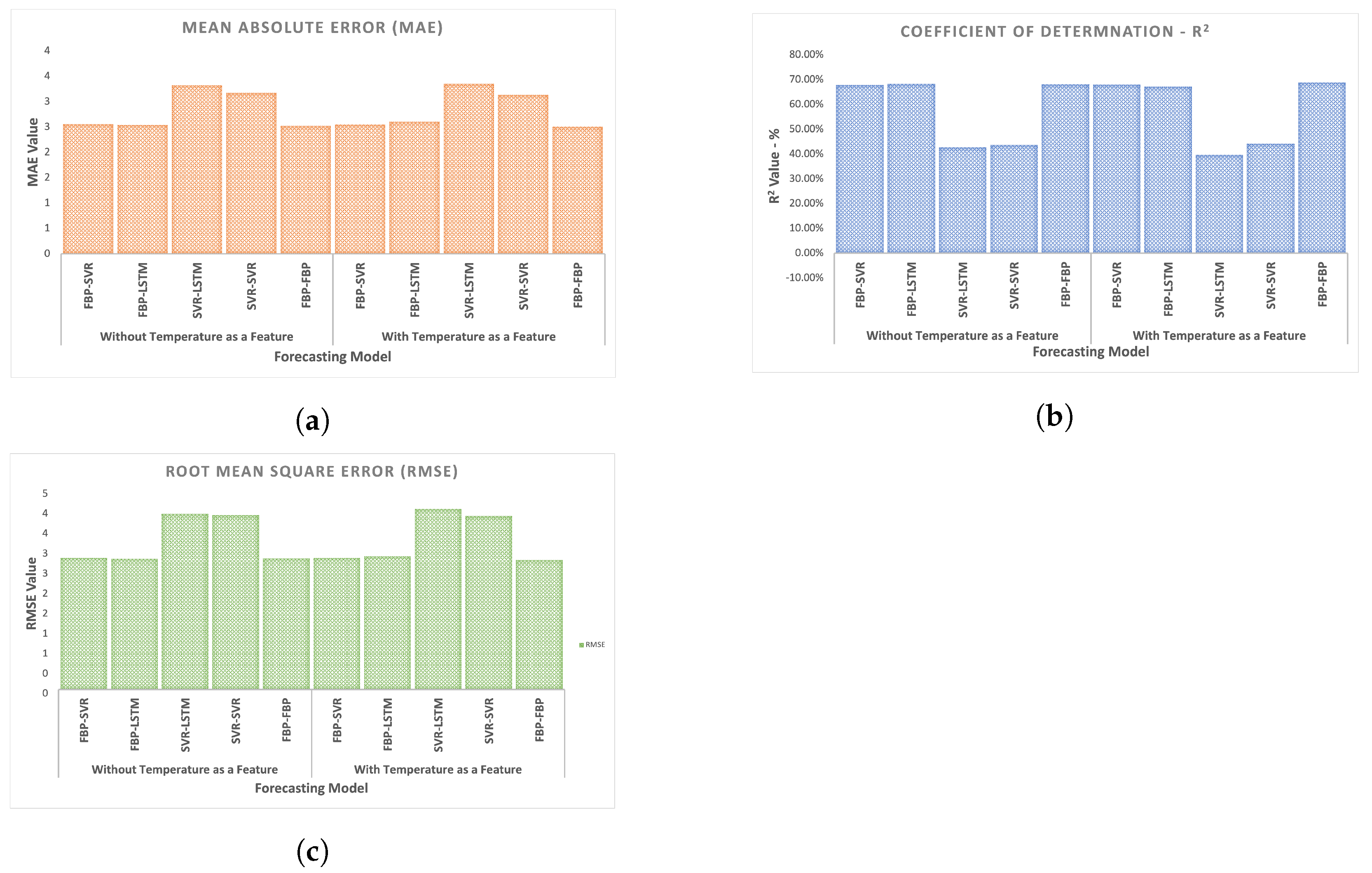
4.2. Multistage Models with Similar Algorithms

As discussed in Section 4.1, the LSTM outperformed the LASSO, SVR, and FBP algorithms. Accordingly, the multistage models are developed to see whether the performance of those models can be improved. For this, we chose to create the multistage models using only the SVR and FBP models, given that the LASSO algorithm gave poor results.
Table 5 and Figure 8 show a performance comparison between the two multistage models constructed from the SVR and the FBP. The results show a significant advantage to the FBP-FBP (with and without consideration of temperature as a feature) compared to all other cases, including the SVR-SVR with and without consideration of temperature and the FBP-FBP with temperature. The recorded metrics are an R 2 value of 68.81 % , an MAE of 2.51 , and an RMSE of 3.25 . Once again, the effect of the temperature is very minor and only accounted for an increase of 0.75 % in accuracy.
The output from the FBP-FBP multistage model without temperature as an extra feature is plotted to visualise the performance (see Figure 9). As can be seen, the slightly poor accuracy reported in the R 2 value of 68.06 % is visually clear in the comparison of the predicted data with the observed/testing data.

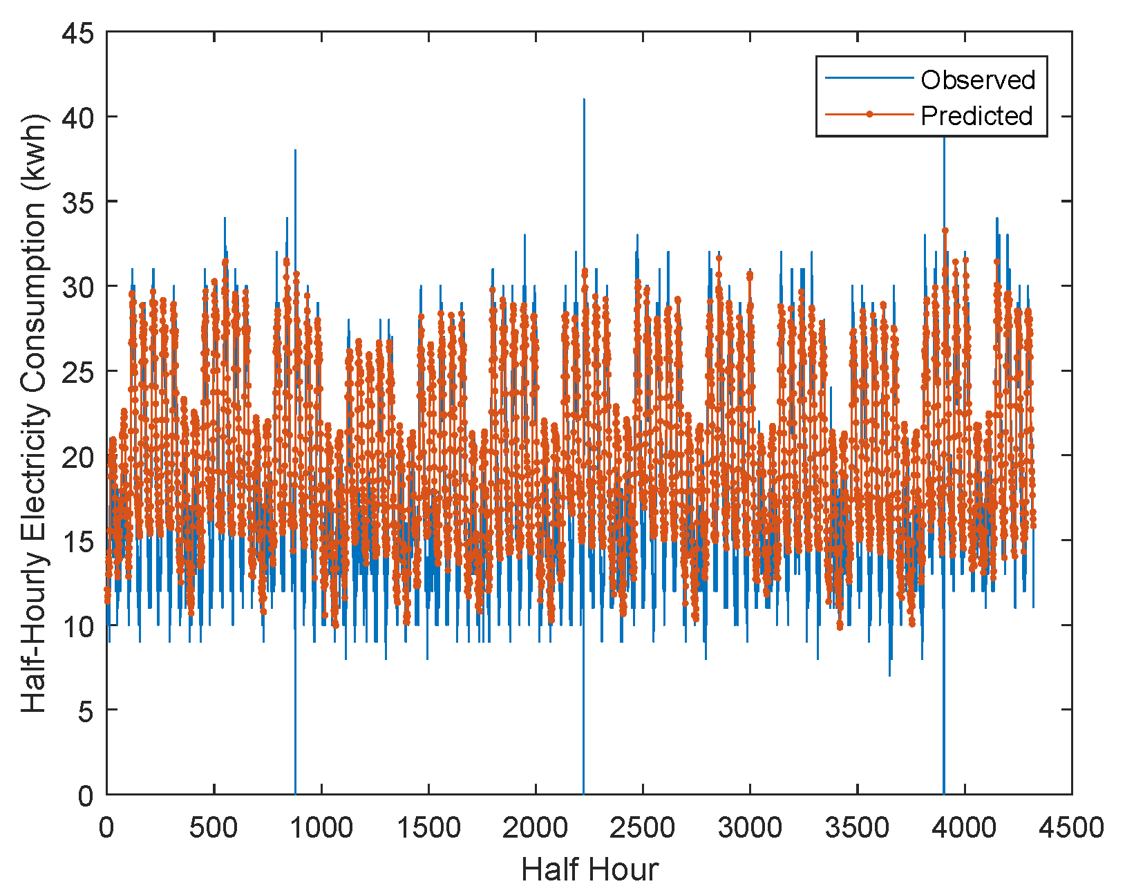
4.3. Multistage Models with Hybrid Algorithms

In this subsection, we present the results of the hybrid models where we used two different forecasting algorithms to enhance the accuracy. Table 6 and Figure 10 show a performance comparison between the two multistage hybrid models constructed from the SVR, FBP, and LSTM. The results show a slight advantage to the FBP-LSTM (without consideration of temperature as a feature) compared to all other models, including the FBP-SVR, and SVR-LSTM, with and without consideration of temperature. The recorded metrics are an R 2 value of 68.22%, an MAE of 2.54, and an RMSE of 3.28.
The output from the FBP-LSTM multistage model is plotted to visualise its performance. As shown in Figure 11, the actual/testing data can be visually identified, especially for values that are less than the mean value and outliers.

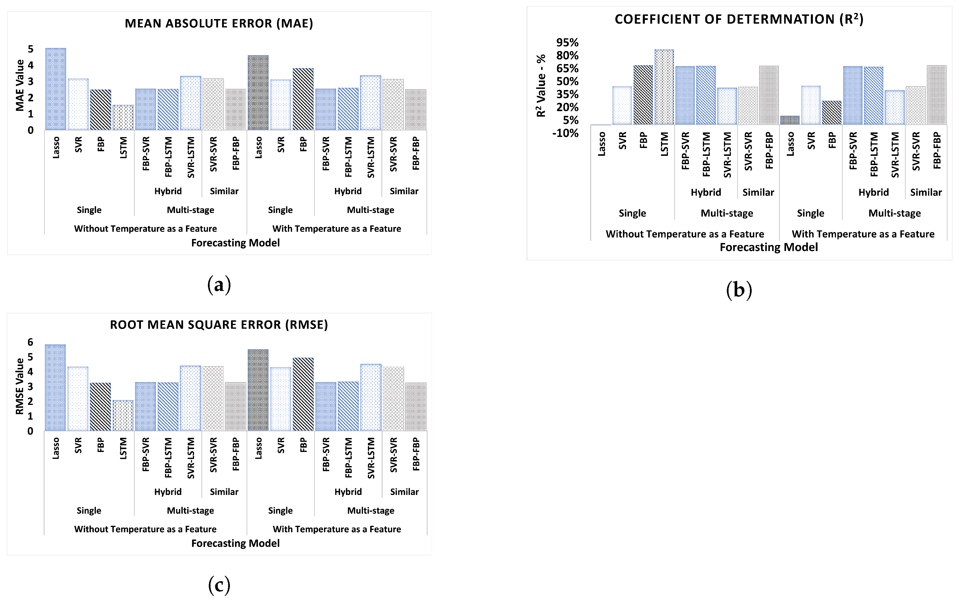
4.4. Evaluation and Discussions

As shown in Table 7 and Figure 12, the forecasting accuracy varies depending on the different models used. We can also observe that the LSTM model has the best accuracy as it can capture the daily consumption pattern. The FBP-FBP is the best performing hybrid model, despite the 68 % accuracy; this can be explained by the ability of FBP to incorporate seasonality (e.g., holidays) into its forecast, and with FBP as the second model, its accuracy can be optimised by taking into account unusual consumption patterns.
To further investigate the success of FBP-FBP, we present the residuals from the first FBP model. From the residual values shown in Figure 13, we can observe that the vast majority of the values lie between −10 and 10, except for the outliers, which can have a major effect on the error values. To better evaluate the residuals, we plotted their histogram in Figure 14. We can observe that the residuals can be modeled as a normal distribution with a relatively narrow variance. Thus, the second FBP would use the residuals and build an accurate forecast, ultimately optimising the accuracy.

5. Conclusions and Future Work

The study presented in this paper considers a total of nine forecasting models, categorised into single and multistage ones. The models are trained twice, that is, with and without consideration of the external temperature as a feature. The results of the comparative study show that the multistage models generally perform better compared to the single models. However, the LSTM stands out and outperforms all other models, and the FBP-FBP model is the best performing multistage model. The results show the edge that recurring neural network models have over all other models, including hybrid models; however, further investigation and fine-tuning of the hybrid models can be done. As far as feature consideration is concerned, the temperature has little or no impact on the results, especially because the high-accuracy results were obtained from the LSTM without using the temperature as a feature, while for the FBP-FBP model, temperature had a minor effect on its accuracy.
For future work, we suggest extending the analysis to a longer time horizon to capture long-term trends, comparing the residual forecasting method to other forecasting techniques, analyzing the impact of demand response strategies, assessing the effectiveness of energy efficiency measures, and exploring the generalisability of the results to other hospital settings and other societal sectors. By conducting these future studies, researchers can gain a more comprehensive understanding of energy demand patterns in hospitals, potential energy-saving strategies, and the applicability of the residual forecasting method in other settings.

Author Contributions

Conceptualization, A.T., B.B., M.M.A.T., C.S.L., M.Z.A. and Q.H.A.; Data curation, A.T.; Formal analysis, A.T., B.B., M.M.A.T. and C.S.L.; Funding acquisition, A.T.; Investigation, A.T.; Methodology, A.T., B.B., M.M.A.T. and C.S.L.; Software, A.T., B.B. and M.Z.A.; Visualization, A.T., M.A.S. and B.B.; Writing—original draft, A.T., B.B., M.M.A.T., M.A.S., C.S.L. and S.H.; Writing—review & editing, A.T., B.B., M.M.A.T., M.A.S., C.S.L., S.H. and Q.H.A. All authors have read and agreed to the published version of the manuscript.

Funding

This research was partially funded by the Engineering and Physical Sciences Research Council (EPSRC) grants, EP/T517896/1.

Data Availability Statement

Restrictions apply to the availability of the electricity consumption data. The data belong to Medway NHS Foundation Trust but were collected using systems provided by EnergyLogix. Data, however, can be made available with the approval of the corresponding author (A.T.), Medway NHS Foundation Trust, and EnergyLogix. As for the weather data, they were obtained from [24].

Acknowledgments

The authors would like to acknowledge the support provided by EnergyLogix and Medway NHS Foundation Trust during the data collection phase. EnergyLogix is a Small to Medium Enterprise (SME) that provided the equipment used for collecting the electricity data for this study. This work was supported in part by the Engineering and Physical Sciences Research Council (EPSRC) grants, EP/T517896/1.

Conflicts of Interest

The authors declare no conflict of interest.

References

  1. NHS. Delivering a ’Net Zero’ National Health Service; Technical Report; National Health Service, NHS England and NHS Improvement: London, UK, 2020. [Google Scholar]
  2. NHS. NHS Energy Efficiency Fund-Final Report; Technical Report; National Health Service: London, UK, 2015. [Google Scholar]
  3. Suganthi, L.; Samuel, A.A. Energy models for demand forecasting—A review. Renew. Sustain. Energy Rev. 2012, 16, 1223–1240. [Google Scholar] [CrossRef]
  4. Hagan, M.T.; Behr, S.M. The Time Series Approach to Short Term Load Forecasting. IEEE Trans. Power Syst. 1987, 2, 785–791. [Google Scholar] [CrossRef]
  5. Fan, J.; McDonald, J. A real-time implementation of short-term load forecasting for distribution power systems. IEEE Trans. Power Syst. 1994, 9, 988–994. [Google Scholar] [CrossRef]
  6. Baliyan, A.; Gaurav, K.; Mishra, S.K. A Review of Short Term Load Forecasting using Artificial Neural Network Models. Procedia Comput. Sci. 2015, 48, 121–125. [Google Scholar] [CrossRef]
  7. Amjady, N. Short-term hourly load forecasting using time-series modeling with peak load estimation capability. IEEE Trans. Power Syst. 2001, 16, 498–505. [Google Scholar] [CrossRef] [PubMed]
  8. Abdel-Aal, R.E.; Al-Garni, A.Z. Forecasting monthly electric energy consumption in eastern Saudi Arabia using univariate time-series analysis. Energy 1997, 22, 1059–1069. [Google Scholar] [CrossRef]
  9. Willis, H.L.; Tram, H.N. Load Forecasting for Trnasmission Planning. IEEE Trans. Power Appar. Syst. 1984, PAS-103, 561–568. [Google Scholar] [CrossRef]
  10. Taylor, S.J.; Letham, B. Forecasting at scale. Am. Stat. 2018, 72, 37–45. [Google Scholar] [CrossRef]
  11. Kong, W.; Dong, Z.Y.; Jia, Y.; Hill, D.J.; Xu, Y.; Zhang, Y. Short-term residential load forecasting based on LSTM recurrent neural network. IEEE Trans. Smart Grid 2017, 10, 841–851. [Google Scholar] [CrossRef]
  12. Siami-Namini, S.; Tavakoli, N.; Namin, A.S. A comparison of ARIMA and LSTM in forecasting time series. In Proceedings of the 2018 17th IEEE International Conference on Machine Learning and Applications (ICMLA), Orlando, FL, USA, 17–20 December 2018; IEEE: Piscataway, NJ, USA, 2018; pp. 1394–1401. [Google Scholar]
  13. Kumar, J.; Goomer, R.; Singh, A.K. Long short term memory recurrent neural network (LSTM-RNN) based workload forecasting model for cloud datacenters. Procedia Comput. Sci. 2018, 125, 676–682. [Google Scholar] [CrossRef]
  14. Dhiman, H.S.; Deb, D.; Guerrero, J.M. Hybrid machine intelligent SVR variants for wind forecasting and ramp events. Renew. Sustain. Energy Rev. 2019, 108, 369–379. [Google Scholar] [CrossRef]
  15. Chen, Y.; Xu, P.; Chu, Y.; Li, W.; Wu, Y.; Ni, L.; Bao, Y.; Wang, K. Short-term electrical load forecasting using the Support Vector Regression (SVR) model to calculate the demand response baseline for office buildings. Appl. Energy 2017, 195, 659–670. [Google Scholar] [CrossRef]
  16. Ekonomou, L.; Christodoulou, C.A.; Mladenov, V. A short-term load forecasting method using artificial neural networks and wavelet analysis. Int. J. Power Syst. 2016, 1, 64–68. [Google Scholar]
  17. Karampelas, P.; Vita, V.; Pavlatos, C.; Mladenov, V.; Ekonomou, L. Design of artificial neural network models for the prediction of the Hellenic energy consumption. In Proceedings of the 10th Symposium on Neural Network Applications in Electrical Engineering (NEUREL 2010), Belgrade, Serbia, 23–25 September 2010; IEEE: Piscataway, NJ, USA, 2010; pp. 41–44. [Google Scholar]
  18. Stratigakos, A.; Bachoumis, A.; Vita, V.; Zafiropoulos, E. Short-term net load forecasting with singular spectrum analysis and LSTM neural networks. Energies 2021, 14, 4107. [Google Scholar] [CrossRef]
  19. Aravazhi, A. Hybrid Machine Learning Models for Forecasting Surgical Case Volumes at a Hospital. AI 2021, 2, 512–526. [Google Scholar] [CrossRef]
  20. Bagnasco, A.; Fresi, F.; Saviozzi, M.; Silvestro, F.; Vinci, A. Electrical consumption forecasting in hospital facilities: An application case. Energy Build. 2015, 103, 261–270. [Google Scholar] [CrossRef]
  21. Tsakoumis, A.C.; Vladov, S.S.; Mladenov, V.M. Electric load forecasting with multilayer perceptron and Elman neural network. In Proceedings of the 6th Seminar on Neural Network Applications in Electrical Engineering, Belgrade, Yugoslavia, 26–28 September 2002; IEEE: Piscataway, NJ, USA, 2002; pp. 87–90. [Google Scholar]
  22. Barakat, B.; Taha, A.; Samson, R.; Steponenaite, A.; Ansari, S.; Langdon, P.M.; Wassell, I.J.; Abbasi, Q.H.; Imran, M.A.; Keates, S. 6G Opportunities Arising from Internet of Things Use Cases: A Review Paper. Future Internet 2021, 13, 159. [Google Scholar] [CrossRef]
  23. EnergyLogix. EnergyLogix Software, Helping to Manage Energy Consumption Information. 2019. Available online: https://energylogix.com/energy-monitoring/software/ (accessed on 9 February 2023).
  24. Science and Knowledge Service. JRC Photovoltaic Geographical Information System (PVGIS)-European Commission. 2020. Available online: https://europa.eu/capacity4dev/afretep/wiki/pvgis-photovoltaic-geographical-information-system (accessed on 9 February 2023).
  25. Wang, Y.; Shen, Y.; Mao, S.; Chen, X.; Zou, H. LASSO and LSTM Integrated Temporal Model for Short-Term Solar Intensity Forecasting. IEEE Internet Things J. 2019, 6, 2933–2944. [Google Scholar] [CrossRef]
  26. Chai, T.; Draxler, R.R. Root mean square error (RMSE) or mean absolute error (MAE)?–Arguments against avoiding RMSE in the literature. Geosci. Model Dev. 2014, 7, 1247–1250. [Google Scholar] [CrossRef]
Figure 1. Violin plot showing descriptive statistics of the electricity demand in the five areas considered in the study.
Futureinternet 15 00134 g001
Figure 2. Violin plot of the typical meteorological year temperature and the half-hourly energy consumption.
Futureinternet 15 00134 g002
Figure 3. Splitting of the data into training and testing periods.
Futureinternet 15 00134 g003
Figure 4. Architecture of the multistage model.
Futureinternet 15 00134 g004
Figure 5. Data flow through the multistage model.
Futureinternet 15 00134 g005
Figure 6. MAE, R 2 , and RMSE values for the single models with and without temperature as a feature. (a) Mean Absolute Error (MAE). (b) Coefficient of Determination ( R 2 ). (c) Root Mean Square Error (RMSE).
Futureinternet 15 00134 g006
Figure 7. Testing data vs LSTM forecasted data of the hospital’s electricity demand.
Futureinternet 15 00134 g007
Figure 8. MAE, R 2 , and RMSE values for the multistage similar models with and without temperature as a feature. (a) Mean Absolute Error (MAE). (b) Coefficient of Determination ( R 2 ). (c) Root Mean Square Error (RMSE).
Futureinternet 15 00134 g008
Figure 9. Testing data vs forecasted data from Multistage Similar model with FBP of the hospital’s electricity demand.
Futureinternet 15 00134 g009
Figure 10. MAE, R 2 , and RMSE values for the multistage hybrid models with and without temperature as a feature. (a) Mean Absolute Error (MAE). (b) Coefficient of Determination ( R 2 ). (c) Root Mean Square Error (RMSE).
Futureinternet 15 00134 g010
Figure 11. Testing data vs forecasted data from Multistage Hybrid model, with FBP as first model and LSTM as second model, of the hospital’s electricity demand.
Futureinternet 15 00134 g011
Figure 12. Results of the comparative study showing the MAE, R 2 , and RMSE values of all models. (a) Mean Absolute Error (MAE). (b) Coefficient of Determination ( R 2 ). (c) Root Mean Square Error (RMSE).
Futureinternet 15 00134 g012
Figure 13. Values of residuals.
Futureinternet 15 00134 g013
Figure 14. Histogram of residuals.
Futureinternet 15 00134 g014
Table 1. Advantages and Disadvantages of the Different Types of Forecasting Models Commonly Used in the Literature.
Forecasting TechniquesAdvantagesDisadvantages
Time Series Models
(FBP, LSTM, SVR)
Easy to implement and interpret.
Effective in dealing with
strong seasonal effects.
Cannot capture complex relationships
and nonlinearities in the data.
Limited accuracy in long-term forecasting.
Regression ModelsEasy to interpret and implement.
Can capture linear relationships
between variables.
Cannot capture nonlinear relationships
in the data.
Limited accuracy in long-term forecasting.
Econometric ModelsCan capture complex relationships
and nonlinearities in the data.
Can be difficult to interpret and implement.
Limited accuracy in long-term forecasting.
Genetic AlgorithmsCan capture complex relationships
and nonlinearities in the data.
Can optimise multiple objectives
simultaneously.
Can be computationally expensive
and difficult to interpret.
Limited accuracy in long-term forecasting.
Table 2. Advantages and Disadvantages of Specific Techniques/Algorithms Used in the Literature.
AlgorithmAdvantagesDisadvantages
FBPSimple and easy to implement.Limited ability to capture complex patterns in data.
Can perform poorly when there are abrupt changes or
irregularities in the data.
LSTMCapable of capturing long-term dependencies in data.Can be computationally expensive and require large
amounts of data for training.
Can be computationally expensive and require large amounts of data for training.Can be sensitive to the choice of kernel function.
Able to handle nonlinear relationships between variables.Can overfit if not properly regularised.
SVRCan handle nonlinear relationships between variables.Can be computationally expensive and require large
amounts of data for training.
Able to capture complex patterns in data.Can be sensitive to the choice of kernel function.
RNNCapable of capturing long-term dependencies in data.Can be computationally expensive and require large
amounts of data for training.
Able to handle nonlinear relationships between variables.Can suffer from the vanishing gradient problem.
ANNCan handle complex, nonlinear relationships between variables.Can be computationally expensive and require large
amounts of data for training.
Can suffer from the vanishing gradient problem.
ARIMASimple and widely used. Capable of capturing short-term dependencies in data.Limited ability to capture long-term dependencies and
nonlinear relationships between variables.
Can perform poorly when there are abrupt changes or
irregularities in the data.
SARIMAExtends ARIMA to handle seasonal patterns in data.Limited ability to capture long-term dependencies and
nonlinear relationships between variables.
Can perform poorly when there are abrupt changes or
irregularities in the data.
LASSOAble to handle high-dimensional data.Can be sensitive to the choice of regularisation parameter.
Can perform feature selection and help with model interpretability.May not perform well when there are nonlinear
relationships between variables.
MLPAble to handle complex, nonlinear relationships between variables.Can be sensitive to the choice of activation function.
Capable of capturing long-term dependencies in data.Can suffer from the vanishing gradient problem.
Can be used for both regression and classification problems.Can be computationally expensive and require large
amounts of data for training.
Can suffer from the vanishing gradient problem.
May require careful tuning of hyperparameters to prevent overfitting.
Table 3. The typical meteorological year data.
Year201120152012201620152015201220122011201220152012
Month123456789101112
Table 4. Forecasting performance results for all single models: R 2 , MAE, and RMSE values.
Model R 2 MAERMSE
Without
Temperature
as a Feature
SingleLASSO−0.76%5.055.83
SVR44.35%3.174.34
FBP68.68%2.513.25
LSTM87.20%1.552.08
With
Temperature
as a Feature
SingleLASSO10.15%4.615.51
SVR44.99%3.124.31
FBP27.61%3.824.94
Table 5. Forecasting performance results for all multistage similar models: R 2 , MAE, and RMSE values.
Model R 2 MAERMSE
Without
Temperature as a Feature
Multistage
Similar
SVR-SVR43.57%3.174.37
FBP-FBP68.06%2.523.28
With
Temperature as a Feature
Multistage
Similar
SVR-SVR44.14%3.134.34
FBP-FBP68.81%2.513.25
Table 6. Forecasting performance results for all multistage hybrid models: R 2 , MAE, and RMSE values.
Model R 2 MAERMSE
Without
Temperature
as a Feature
Multistage
Hybrid
FBP-SVR67.86%2.563.29
FBP-LSTM68.22%2.543.28
SVR-LSTM42.70%3.324.40
With
Temperature
as a Feature
Multistage
Hybrid
FBP-SVR67.97%2.553.29
FBP-LSTM67.13%2.603.33
SVR-LSTM39.62%3.354.52
Table 7. Forecasting performance results for all models: R 2 , MAE, and RMSE values.
Model R 2 MAERMSE
Without
Temperature
as a Feature
SingleLASSO−0.76%5.055.83
SVR44.35%3.174.34
FBP68.68%2.513.25
LSTM87.20%1.552.08
Multistage
Hybrid
FBP-SVR67.86%2.563.29
FBP-LSTM68.22%2.543.28
SVR-LSTM42.70%3.324.40
Multistage
Similar
SVR-SVR43.57%3.174.37
FBP-FBP68.06%2.523.28
With
Temperature
as a Feature
SingleLASSO10.15%4.615.51
SVR44.99%3.124.31
FBP27.61%3.824.94
Multistage
Hybrid
FBP-SVR67.97%2.553.29
FBP-LSTM67.13%2.603.33
SVR-LSTM39.62%3.354.52
Multistage
Similar
SVR-SVR44.14%3.134.34
FBP-FBP68.81%2.513.25
Disclaimer/Publisher’s Note: The statements, opinions and data contained in all publications are solely those of the individual author(s) and contributor(s) and not of MDPI and/or the editor(s). MDPI and/or the editor(s) disclaim responsibility for any injury to people or property resulting from any ideas, methods, instructions or products referred to in the content.

