1. Introduction
Recent decades represent a huge evolution of Automated Manufacturing Systems (AMS), previously named Flexible Manufacturing Systems (FMS). We can even talk about the new industrial revolution. According to [
1], this evolution is realized mainly by the development in four axes, namely products, technology, business strategies, and production paradigms. The edited book [
2] offers a wide perspective on modern design and operation of production networks. The evolution of the manufacturing system in the future is presented in [
3].
The operation of AMS often has a similar character to Discrete-Event Systems (DES), where the next state depends only on both the current state and the occurrence of discrete events. Petri nets (PN) [
4,
5] are frequently used for modeling and control of DES. The family of AMS is a typical representative of DES where many devices cooperate together—robots, machine tools, transport belts, automatically guided vehicles (AGV), etc. They are frequently called to be resources. They are shared by multiple production lines, robotized working cells, etc. These devices and their aggregates, in the form of lines and cells, can also be considered industrial agents and the whole AMS as a multi-agent system. The adequate resource allocation is very important in AMS in order to avoid deadlocks. A deadlock in general is a state in which two or more processes are each waiting for the other one to execute, but neither can go on. Hence, deadlock is undesirable and bad phenomenon. Due to deadlocks, either the entire plant or some of its parts remain stagnate. Thus, the primal intention of the production cannot be achieved. For a design of deadlock-free AMS discrete mathematics is necessary. PN-based discrete mathematical models of AMS yield a suitable background for this.
There exists a large number of publications interested in this topic. From the older ones, the following works should be mentioned in particular [
6,
7,
8,
9,
10], as well as the UML (Unified Modeling Language)-based work [
11] applied in software engineering. While in [
6,
9] foundations of the
P-invariant-based method were laid, in [
7,
8] the method based on siphons and traps was elaborated. A generalized view on deadlocks in multi-agent systems is presented in [
10]. Among the more recent works should be mentioned [
12,
13,
14,
15], as well as the author’s survey article [
16]. While in [
12] a comprehensive survey of Petri net siphons were presented, in [
13,
15] unreliable resources are investigated and the robust control for AMS containing such resources is designed. In [
14], deadlocks in mobile agent systems are detected and resolved.
In relation to the elimination of deadlocks, in [
16,
17,
18,
19,
20,
21] three categories of strategies are distinguished: (i) deadlock detection and recovery—which is used in cases where deadlocks are infrequent and their consequences are not too serious; (ii) deadlock prevention—it imposes restrictions on the interactions among resources and their users to prevent resource requests that may lead to deadlocks; and (iii) deadlock avoidance—it grants a resource to a user only if the resulting state is not a deadlock.
Consequently, it is impossible to address to such a broad issue in one paper. In this paper, only two methods of deadlock prevention in AMS by means of PN-based models are introduced and compared. Both methods add monitors (additional places) into the original PN model of AMS in order to remove deadlocks. One method enumerates monitors and their interconnections with the original PN model using P-invariants and the other using siphons and traps.
1.1. Formal Methods in AMS
Formal methods for modeling, simulation, supervisory control, performance evaluation and fault diagnosis of AMS are very important part of global understanding of AMS. They yield an efficient help and knowledge at constructing and real implementation of AMS. A suitable review of such methods is presented in the e-book [
22]. As to modeling AMS there are presented also models based on place/transition Petri nets (P/T PN), timed Petri nets (TPN), and hybrid Petri nets (HPN).
The supervisory control of AMS determined for the deadlock prevention and avoidance are presented by means of: (i) finite state automata (FSA); (ii) the Petri net view on AMS which are perceived as resource allocation systems (RAS); (iii) HPN-based inventory control systems; (iv) stochastic flow models (SFM); (v) the infinitesimal perturbation analysis (IPA); and (vi) the max-plus algebra.
The performance evaluation is watched by colored TPN, by continuous PN (CPN), by the timed process algebra, and by the Petri net-based complex system scheduling.
The fault diagnosis of AMS is analyzed by means of FSA, by the fault diagnosis of PN and by the control reconfiguration of discrete-event manufacturing systems modeled by non-deterministic input/output (I/O) automata.
Along with the development of information technologies, such as cloud computing, mobile Internet, information acquisition technology, and big data technology, traditional engineering knowledge and formal methods for knowledge-based software engineering undergo fundamental changes. Hence, networks also play an increasingly important role.
Within this context, it is necessary to develop new methodologies as well as technical tools for network-based approaches. The term “network” may have different meanings in different contexts. To resolve bottleneck problems in AMS, deadlock prevention and avoidance by means of Petri nets is crucial.
Although introduced topics cover a large set of formal methods in AMS it cannot be said that this set is complete. New methods are under development.
1.2. Agents Cooperation, Negotiation and Reentering in AMS
Important strategies in MAS (multi-agent systems) are cooperation and negotiation. A structural and Petri net-based approach to modeling of these strategies was elaborated in author’s older work [
23] and in the chapter [
24] where also the perspectives of learning in this area were analyzed.
In [
25], a connection of the structural model of reenterable AMS on a computer-based supervisory controller for monitoring the status of jobs and regulating the part routing as well as the machine job selection by means of siphons of Petri nets as to resolving deadlocks was explored. Namely, there are many approaches to modeling and analysis of manufacturing systems. In addition to those ones mentioned above in the previous Subsection (i.e., automata, Petri nets, perturbation methods) there exist methods based on digraphs, alphabet-based approaches, control theoretic techniques, expert systems design, etc.
The so-called complex networks are an interdisciplinary area. Numerous natural and artificial systems are composed of a large number of individuals that interact with each other in various ways, and then perform surprising useful functions. Examples of such networks include, e.g., neural networks, social networks, and many others, but also MAS in general, including industrial MAS where AMS and RAS belong, and doubtlessly also PN that successfully model and analyze them.
1.3. The Paper Organization
In the following
Section 2, preliminaries concerning theory of PN and the PN-based modeling of AMS will be concisely introduced. Then,
Section 3 will be devoted to the presentation and illustration of the method of deadlock prevention, based on P-invariants. In
Section 4, the method of deadlock prevention, based on PN siphons and traps, will be presented and illustrated.
Section 5 will discuss and illustrate three PN models of AMS being more complicated from the computation point of view, namely problematic because of very long-lasting even impossible computations. In
Section 6, the comparison of both methods will be introduced. Then,
Section 7 contains a concise conclusions of this paper.
2. Preliminaries
Firstly, it is necessary to introduce several basic definitions. First, one is the author own definition extracted from knowledge published in [
7,
16], next three are the standard elementary definitions of
P-invariants, siphons, and traps from the classical literature about Petri nets [
4,
5]. Last two definitions are taken over from [
7].
Definition 1. A Petri net is a bipartite directed graph (BDG). It may be formally described by the quadruplet . Here, P and T are finite nonempty sets, namely P is a set of places (), representing the first kind of BDG nodes, and T is a set of transitions (), representing the second kind of BDG nodes. It is valid that and . The set is the flow relation of the net N. It is expressed by directed arcs from places to transitions and vice versa. The mapping assigns weights to directed arcs. The weight of an arc f: if and otherwise. Here , i.e., it contains natural numbers plus zero. The Petri net is named ordinary and denoted as if . N is called generalized if . Petri net is called a state machine if, and only if, (iff) , i.e., when each transition has only one input place and only one output place.
A mapping from P to is a marking M of N. The marking means the number of tokens located in the place p. Thus, we may say that the place p is marked by a marking M iff . In case of a subset we say that it is marked by M iff at least one place in S is marked by M. The sum of tokens located in all places of S is . S is empty at M iff . The pair is called the marked net or a net system. Here, is an initial marking of N.
PN marking is evolved as follows
with
being the
initial marking. Here,
is the
-dimensional incidence matrix based on the set
F and
is a
-dimensional firing vector (the binary vector, where its entry with the value 1 denotes the corresponding transition
able to be fired).
denotes (as it was already mentioned above) the number of tokens in place
p.
marking vectors
are sometimes named also as
state vectors.
, where
and
are, respectively, the output flow matrix and the input flow matrix. In other words, the matrix representing the output of transitions to places and the matrix representing the input of places to transitions.
For economy of space, in general, markings and vectors can be described by the formal sum notation. Thus, denotes the vector . For example, in a net with a marking where in are 3 tokens and in are 2 tokens may be written as instead of the vector notation .
Definition 2. A vector is a place invariant P (shortly, P-invariant) of PN iff and . Here, is the incidence matrix of N.
Definition 3. Any set with is said to be a siphon. Verbally said, if every transition having an output place in S has an input place in S. If a siphon does not contain another siphon, being its proper subset, it is said to be a minimal siphon. A proper subset is any subset of the set except itself. A minimal siphon S is called a strict minimal siphon (SMS) if . In other words, if there is no siphon contained in it as a proper subset. A SMS does not contain a trap (the trap is defined below by Definition 4). When at the initial marking , S is called an empty siphon.
Definition 4. Any set with is called a trap. In other words, if every transition having an input place in Q has an output place in Q.
Definition 5. A siphon S is said to be controlled in a net iff . Here, expresses the reachability of markings from the initial marking. Consequently, any siphon containing a marked trap is controlled, since the marked trap can newer be emptied. Thus, in ordinary PN a controlled siphon does not cause any deadlock.
Definition 6. A siphon S in an ordinary PN is [7] invariant controlled by P-invariant under the initial marking iff and , or equivalently, and . Here, is the positive support of . Here, it is necessary to notify and emphasize that both methods examined in this paper require a rather wide mathematical background that cannot be either simplified nor abbreviated. Otherwise, the integrity of the interpretation of the methods would be violated. The mathematics used in examples should contribute to an accurate understanding of the application of both methods to particular cases of AMS.
2.1. Petri Nets and Resource Allocation Systems
Resource allocation systems (RAS) are a special class of concurrent systems, especially AMS. There, the attention is focused above all on resources. The set of Petri net-based models of RAS represent, in general, a subset of complete set of PN. Finite set of resources is shared in a competitive way by a finite set of processes. Such a competition induces (or may induce) existence of deadlocks. PN-based models of RAS are useful at synthesizing policies of deadlock prevention and/or deadlock avoiding. They make possible to design beforehand deadlock-free AMS, what is very useful especially preliminary to the creation of the final design of the structure of real AMS determined for application in production.
There are several standard paradigms of RAS [
26,
27,
28,
29]. Specific nomenclatures have been established for them—see, e.g., a survey made in [
16], where also their mutual relations and their relations to PN as a whole, are displayed. Most frequently used paradigms of them are the following two: (i) S
3PR (
Systems of
Simple
Sequential
Processes with
Resources) suitable for AMS with flexible routing and the acquisition of the single-unit of the resource and (ii) S
4PR (
System of
Sequential
Systems with
Shared
Process
Resources) which enables the modeling AMS with flexible routing and the acquisition of more units of the resource. The relation S
3PR ≺ S
4PR in this case expresses that systems S
4PR model more complicated AMS than systems S
3PR are able to model. In future, there may be S*PR (S
3PR ≺ S
4PR ≺ S*PR) paradigms suitable to model of yet more complicated AMS, where yet more copies of resources will be allowed. However, the asterix needs not always be just a greater integer than it was in previous two paradigms.
Some of the amount of paradigms, especially S
3PR and S
4PR, can be modeled and simulated in Matlab by means of the tool [
30].
2.2. Methods for the Deadlock Prevention and Avoiding
As already mentioned, two main streams of methods are represented by methods based on: (i) reachability trees and P-invariants of PN and (ii) PN siphons and traps.
In the former case, it is necessary to mention the most principal contributions [
6,
8,
9,
31,
32,
33] important for the evolution of the
P-invariants-based methods. The origin of this method consists in the effort to deal with the problem of the forbidden state in DES. Namely, it was shown in the literature that if a set
of legal PN markings is expressed by a set of
s linear inequality constraints (so called General Mutual Exclusion Constraints (GMEC)) and if
is controllable, then the PN-based solution exists and it is maximally permissive. The controllability of
means that from any marking
no forbidden marking is reachable by firing a sequence containing only uncontrollable transitions. In the opposite case, a general forbidden marking constraint may be enforced by PN-based controller only if the Petri net model of the system is safe. Hence, PN
P-invariants are used in order to compute the feedback controller that enforces GMEC. They perform transformations on the system’s specifications to obtain constraints in the desired form. The controller is a set of control Petri net places. When the controller is added to the PN model of the plant, control places ensure a live and maximally permissive behavior of the closed loop system with respect to the forbidden states or markings. The controller design has a linear complexity in the number of system states. However, there are cases where such PN controller does not exist. Especially, when the set of legal markings
is not convex, there does not exist any PN place that can forbid the reachability of bad markings when allowing all legal ones. The concept of PN
P-invariants was extended also to PN with uncontrollable and unobservable transitions. However, in this case maximally permissiveness cannot be guaranteed.
In the latter case, there are lots more such basal publications—[
6,
7,
10,
28,
34,
35,
36,
37,
38,
39,
40,
41,
42,
43,
44,
45,
46,
47,
48,
49,
50,
51,
52,
53,
54,
55,
56,
57]. Siphons are tied to dead transitions whose existence leads to the loss of liveness of PN-based models of AMS. Siphon control is an effective way to prevent the occurrence of deadlocks. In a general case, particularly for models of AMS based on generalized PN, a siphon-based deadlock prevention policy cannot find an optimal (i.e., maximally permissive) supervisor. However, for PN models of AMS based on ordinary PN it is possible. Siphons in the PN model of a plant are divided into elementary and dependent ones. A monitor is added to the plant model for each elementary siphon, in such a way that the siphon will be
invariant-controlled. The method guarantees that no further emptiable control-induced siphon is generated due to the addition of the monitors. When all elementary siphons are controlled, the controllability of a dependent siphon is ensured by properly setting the
control depth variables of its related elementary siphons.
The explanation of the term invariant-controlled siphon, as well as the term control depth variable, will be explained and illustrated below in the
Section 4.2. However, this is applicable only for S
3PR paradigm of RAS. In case of S
4PR paradigm (modeled by generalized PN), which uses multiple resource requirements and information about the weight of arcs, the concept of extended elementary siphons have to be used. Namely, due to the complicated utilization of resources, it is insufficient to represent the relationship between elementary and dependent siphons in generalized PN in such way as it is in case of ordinary PN. Extended elementary siphons are find by an iterative process—see, e.g., [
58].
A methodology for modeling and analyzing fault-tolerant manufacturing systems that not only optimizes normal productive processes, but also performs detection and treatment of faults is presented in [
59]. The coordination of cooperative multirobot system by means of PN is elucidated in [
60].
The methodological framework yielded by the S
4PR paradigm of RAS has raised considerable interest [
61] on the grounds of a well-balanced compromise between modeling flexibility and the provision of sound and effective correction techniques.
In [
62], a very general class of Petri nets are defined. This class has been called Petri nets of resource allocation (PNRA) to model as many kinds of RAS as possible. It not only focuses on the resources shared by processes, but also pays attention to the interaction/collaboration among processes.
At the solving of deadlock problems in AMS modeled with PN in [
63], the attention is focused on adding a set of recovery transitions.
Here, in this paper, devoted to deadlock prevention and avoiding, it is not a sufficient space to analyze all introduced literature sources in details item by item. Namely, this area has many isolated particulars which are analyzed in detail in the above literature [
6,
7,
8,
9,
10,
28,
31,
32,
33,
34,
35,
36,
37,
38,
39,
40,
41,
42,
43,
44,
45,
46,
47,
48,
49,
50,
51,
52,
53,
54,
55,
56,
57].
Methods based on P-invariants are divided into many subclasses interested in deterministic and/or unreliable resources, methods suitable for ordinary and/or generalized PN, methods using linear and/or non-linear restrictions, methods applying optimization based on the linear programming (usually mixed integer linear programming (MILP)), etc.
Methods based on siphons and traps have still lots more such subclasses. The very good literature review of methods concerning the deadlock prevention is made in [
26]. Likewise, in [
53] a crucial literature review concerning the deadlock control is presented. A variety of deadlock-control policies is mentioned there. The optimization based on MILP is one of them. Such optimization can eliminate the need to compute completely all elementary siphons, which shorten the computational time for finding indispensably needed siphons.
In the following two sections, principles of both methods of the prevention of deadlocks will be introduced and mathematically described. Illustrative examples explaining the application of both methods in details will be introduced there as well.
3. P-Invariant-Based Method of Prevention Deadlocks
P-invariants are vectors
with the important property. The multiplication of such vectors with any marking (state) vector
reachable from a given initial marking
yields the same result. It is the relation of the state conservation, as follows
Taking into account the consecutive states obtained by firing of only one transition, we have for each transition
t
where,
is the column of the incidence matrix
corresponding to the transition
t. These vectors are solutions of the following equation
what corresponds with the original Definition 2 of
P-invariants introduced in the
Section 2.
Consider the inequality representing linear combinations restricting behavior of marking
Here,
is a matrix of integers,
is an integer vector. An efficient help at creating
yields the reachability tree (RT) of the net
N. After removing inequality by adding slack variables, we have
where entries of the
vector
represents slack variables.
Just the Equation (
4) represents the base of the method for the supervisor synthesis. Namely, when we force there
instead of
, we obtain (
7) and some additional PN places (slacks) can be added to
N. Thus, the extended (augmented) PN
(where the symbol ∘ expresses a composition) will arise.
is the PN which will (after finding its interconnections with
N) ultimately create the supervisor. Then, slacks will create the places of the supervisor, frequently called monitors. In
we have the following structure of (
4) in the form
where
is
-dimensional
identity matrix;
is the number of slacks;
is a
-dimensional matrix which in a suitable form expresses the conditions imposed on marking (state) vectors of the original PN
N, and
is the
-dimensional matrix. After finding
from (
7) by computing, we have the structure of the PN-based model of the supervisor—i.e., interconnecting arcs between
N and
. Consequently, in general,
where
is
and
is
of
.
The marking
of the supervised system
consists of the state vector
of the
N augmented with the state vector
of the supervisor
. Analogically, the incidence matrix
of the net
consists of the incidence matrix
of
N augmented with the incidence matrix
of the net
. The marking and the incidence matrix of the net
are as follows
Here,
,
and
are expressed by sub-matrices
and
,
and
, and
and
.
Because of the prescribed conditions we have
where
is the
)-dimensional vector (see (
5) and (
6)). Its integer entries represent the limits for number of tokens in (
5). Sometimes
where
is the vector with all its entries equal to 1. Because
the initial state vector of the supervisor can be simply computed as follows
Example 1
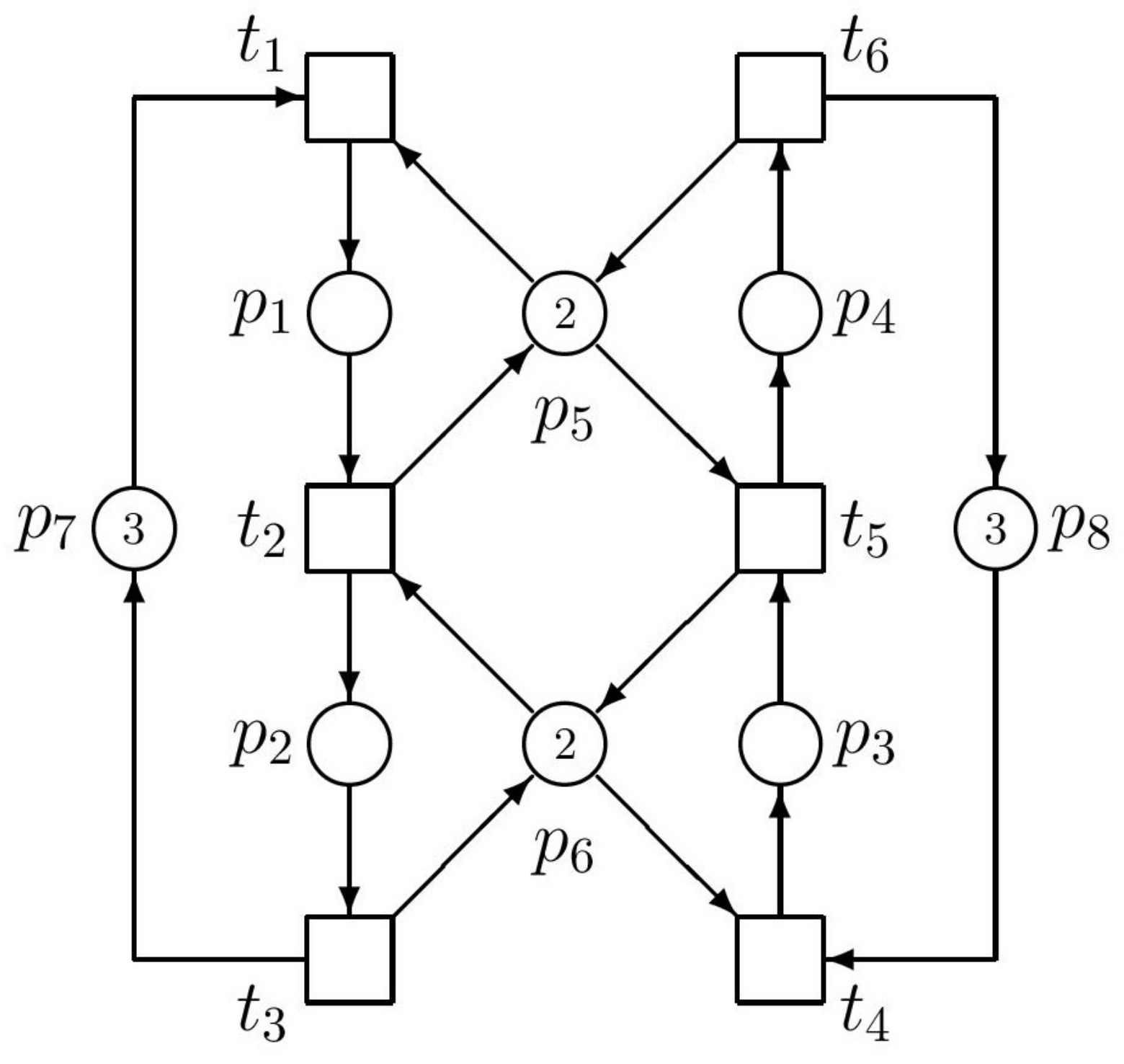
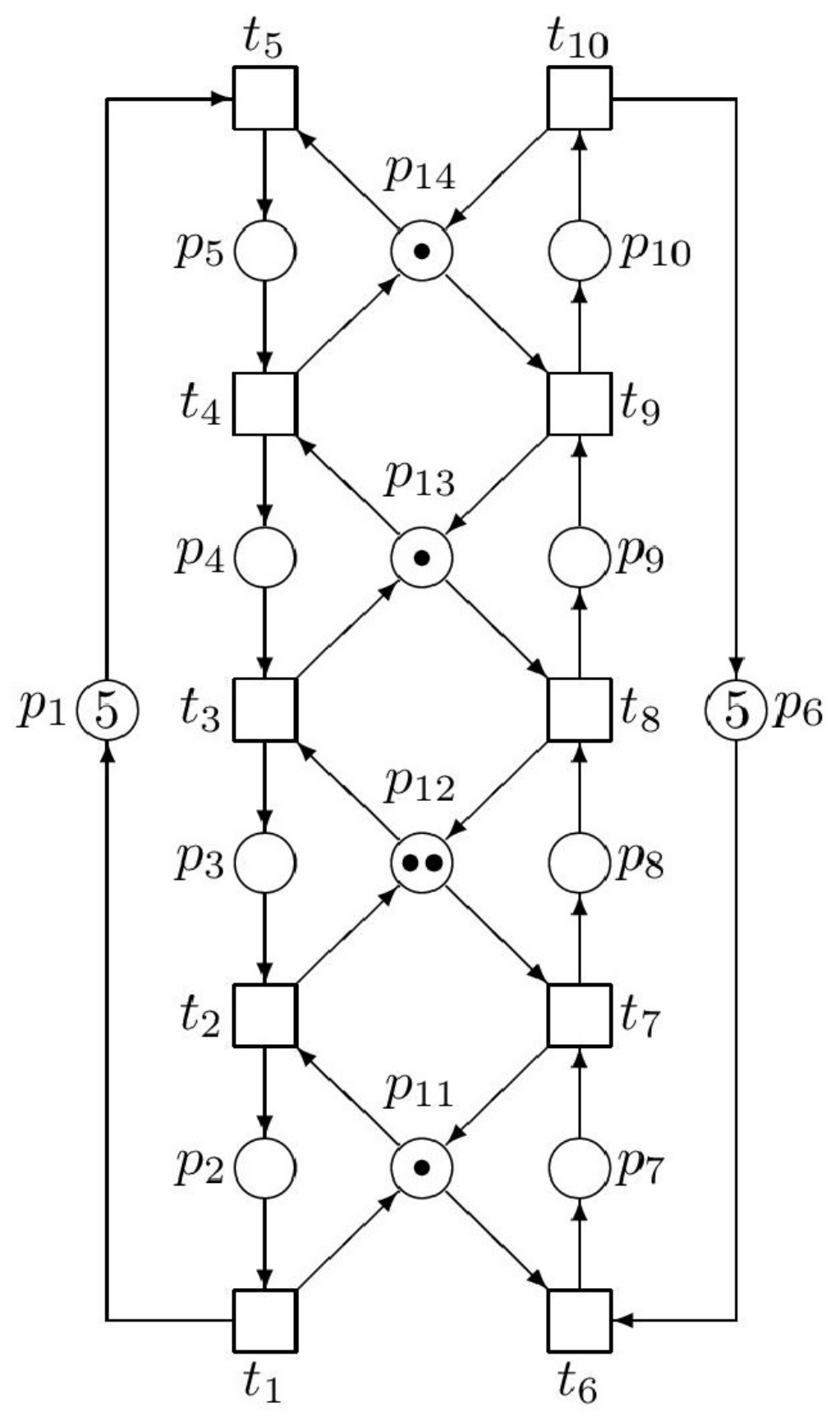
Consider the simple example of
N modeling an AMS with two production lines {
} and {
} with two common resources
and
, introduced in
Figure 1. Places
and
are idle process places,
,
,
, and
are active process places, and
and
are resource places. A token in an active process place models, e.g., a part being processed. In
Figure 1, active process places are empty till firing
and/or
. Tokens located in a resource place model, e.g., the available capacity of buffers. Tokens located in an idle place indicate the maximal number of concurrent activities that can occur in a process represented by the corresponding production line.
Parameters of
N are as follows
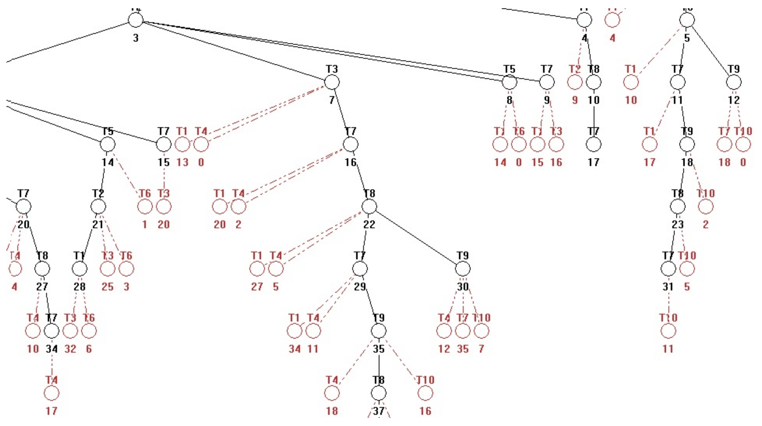
This
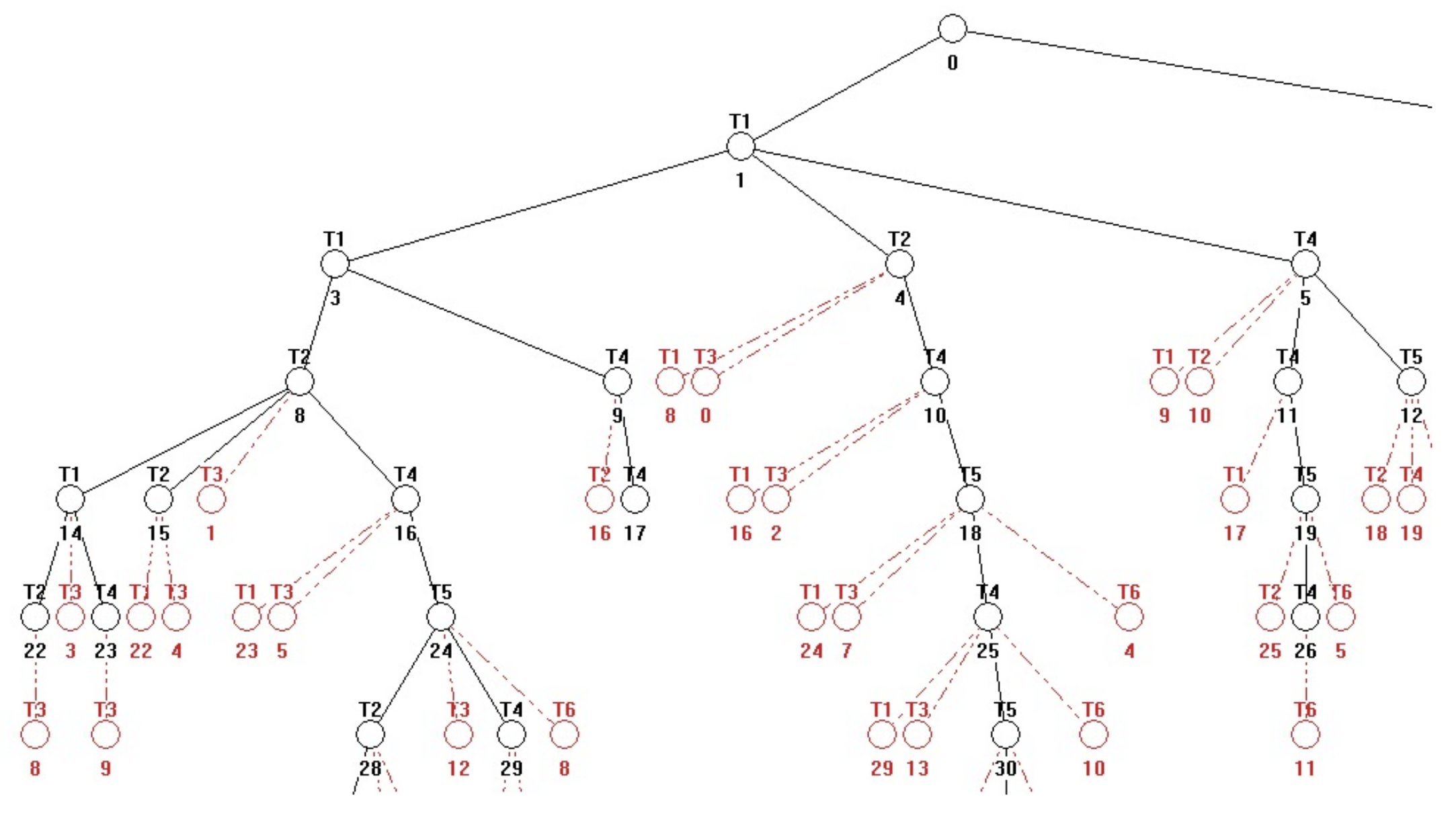
N has, at the given initial state
, the fairly branched (patulous) reachability tree (RT) with 33 nodes (including
). All RT nodes, being the reachable markings
are the columns of the following matrix (in the ascending order):
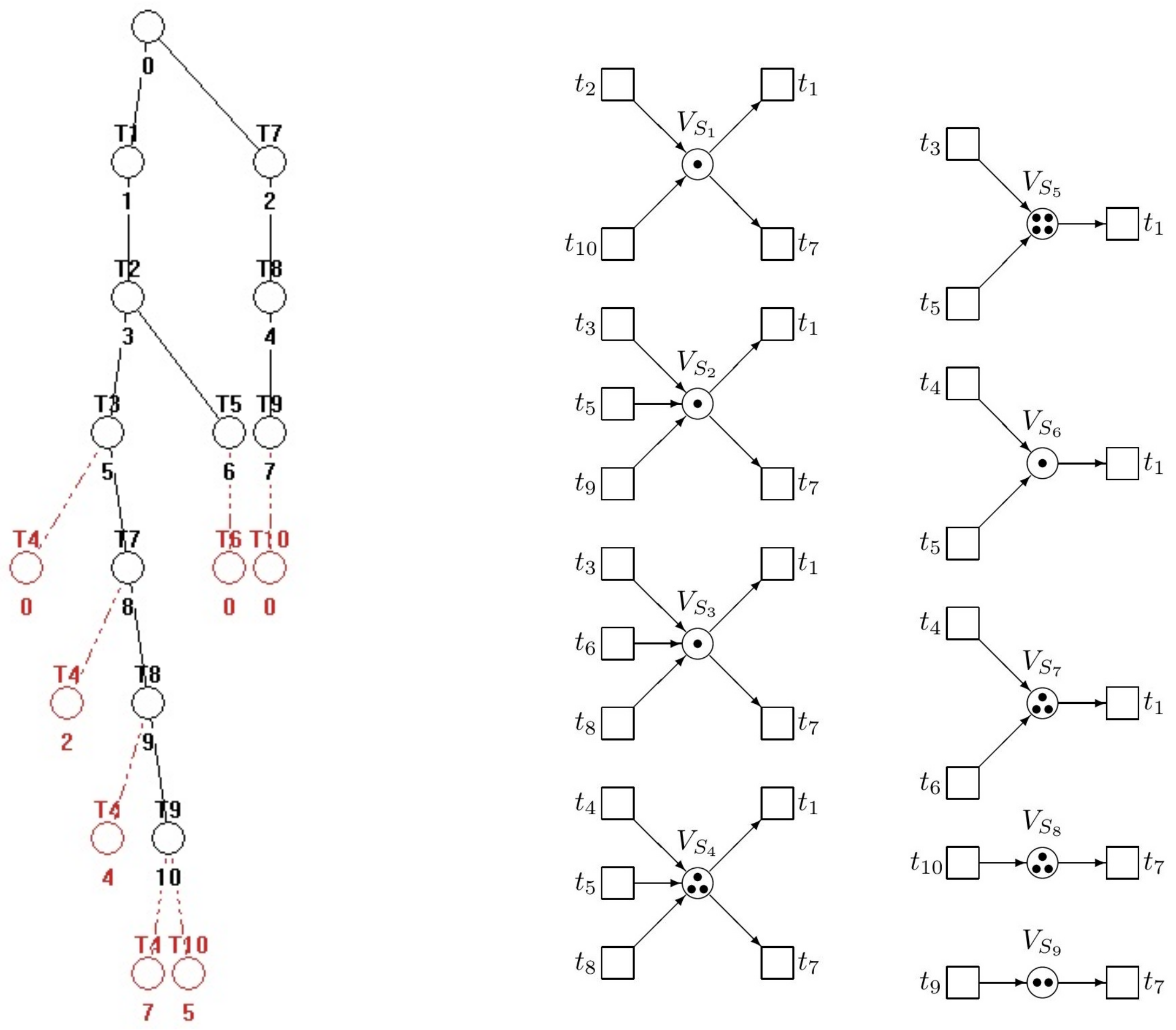
Because RT is too big, it cannot be introduced here full. In
Figure 2, at least its principal fragment is introduced.
From the RT fragment we can find the solitary deadlock
—see (
18), where it is separated. This deadlock can be reached by following paths:
Hence, we can see that in RT the node
immediately precedes the node
representing the deadlock. These nodes are marking vectors
(the 10th column of
because the first column is
) and
(the 18th column of
). After comparing entries of these vectors, from (
19) follows the restriction
(i.e., only one of them can be marked), i.e.,
and
. Consequently,
and
because in (
16)
. Hence, with respect to (
11)–(
13) we have the augmented PN
(i.e., the original uncontrolled net
N together with the net
representing the supervisor) and the augmented vector
of the initial marking as follows
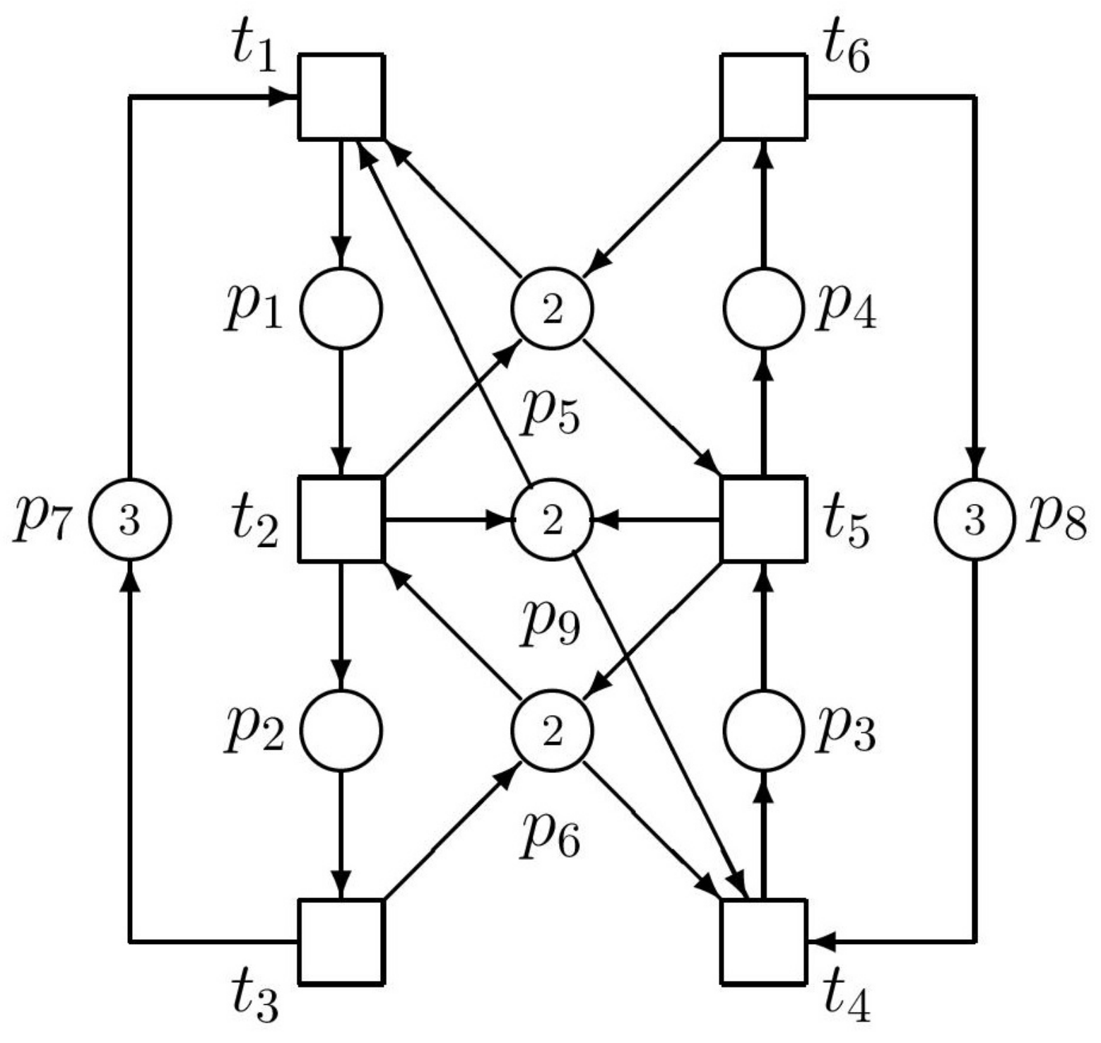
Thus, we have the supervisor represented by the single PN place
(monitor) interconnected with the original PN model as it can be seen in
Figure 3.
After computing RT of the augmented net, we can find that it contains 28 nodes and no deadlock exists there. It means that the augmented net works correctly.
4. Siphon and Trap-Based Method of Prevention Deadlocks
Such approaches are much more widespread than approaches based on P-invariants. There are many sources in literature. Let us mention at least some of them [
7,
8,
12,
13,
16,
29].
Invariants, siphons, and traps are structural entities of PN. All of them can be computed, e.g., by the Matlab-based tool presented in [
30]. The problem of deadlock prevention in a concurrent system represented by
N is equivalent to the problem of avoidance of empty siphons in the ordinary PN model of
N. When at least one empty siphon occurs in ordinary PN
N, the net is totally deadlocked [
5].
At the supervisor synthesis it is sufficient to consider only minimal siphons. It is necessary to ensure that the sum of the number of tokens in each minimal siphon S is never less than one, namely in any reachable marking M. In such a case, the general condition for ith siphon can be replaced by the condition in the form . This can be derived as follows.
Consider the following formal specification in
N
where
is a (
)-dimensional vector,
is a marking and
b is a scalar;
b and the entries of
are integers. The relation (
24) says that the weighted sum of the number of tokens in each place should be greater than or equal to a constant.
In [
6], it was proved that if a Petri net
with incidence matrix
and initial state
satisfies the following relation
then a control place
can be added, that enforces (
24). Let
(
is the set of integers) denotes the weight vector of arcs connecting
with the transitions in the net
N;
is obtained by
. In general, when there are more
than one,
with
being the matrix were rows represent particular
appertaining to particular
. The initial number of tokens in
is
or, in general,
.
The controlled Petri net is maximally permissive. The control process enforces
just enough control to avoid all illegal markings. This is the basis for deadlock prevention, i.e., for the synthesis of the control algorithm based on siphons. Thus, the place invariant guarantees that for any marking
in the set of reachable markings of
NHere, as it was defined above,
is the number of tokens in the control place
. Due to the fact that
is non-negative, the inequality in (
24) is satisfied. Equation (
25) expresses the demand that (
24) must be satisfied for
, otherwise no solution exists there.
represents the row which extends the incidence matrix
of the uncontrolled net
N with respect to the control place
. In general, for more additive places
, it can be written
where
is (
) matrix of positive integers greater than or equal to 0.
has the weighted vectors
,
, as its rows. The vector
is (
) vector of restrictions with entries being positive integers greater than or equal to 0;
is (
) vector of slacks with entries being positive integers greater than or equal to 0. Thus, we obtain the controlled PN model (with the incidence matrix
) consisting of original uncontrolled model (with the incidence matrix
) and the siphon-based controller (with the incidence matrix
) as follows
The controller consists of monitors and their interconnections with the original PN model.
Replacing
by the siphon
, or, in general, replacing
by the matrix of siphons
(where particular siphons are its rows) we obtain
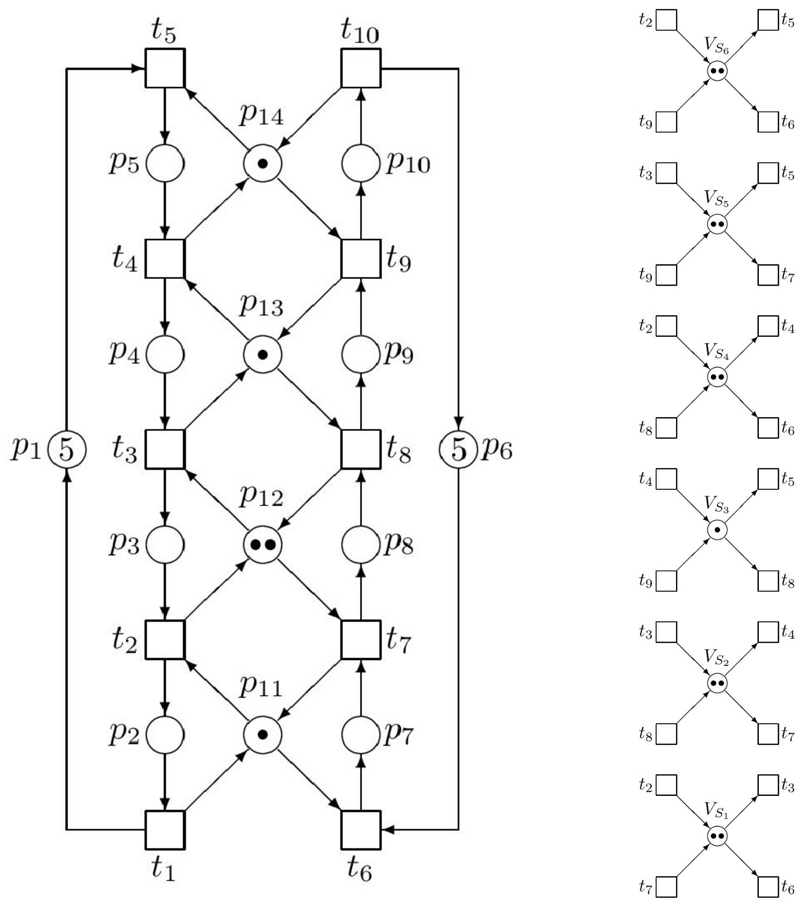
4.1. Example 2
Minimal siphons and traps of the PN model in
Figure 1 are the following
| |
| |
| |
| |
| |
Denote
and
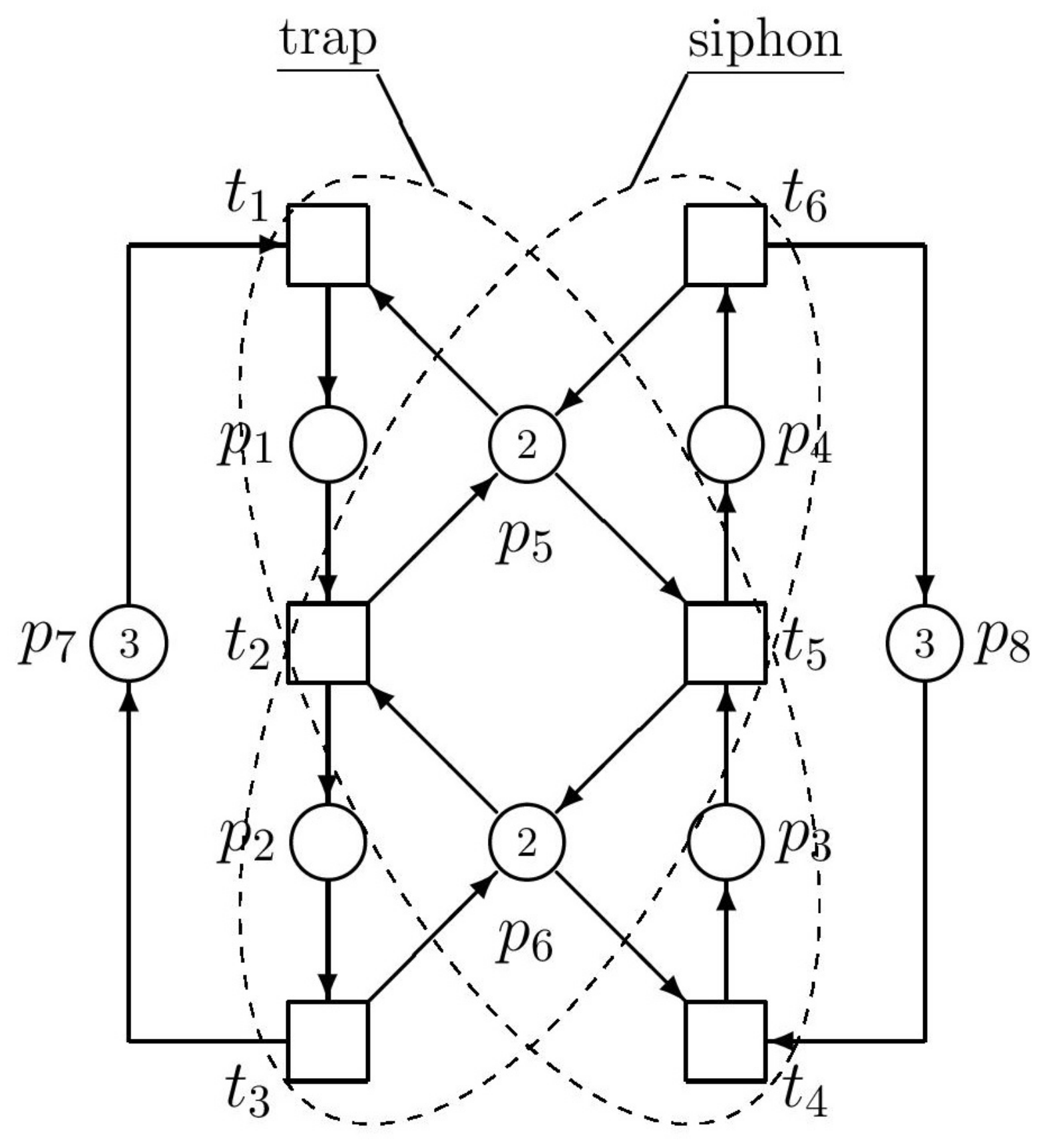
. In this simple example, the siphon and trap can be illustrated by
Figure 4. Above introduced crossed siphons are equaled to traps. Such a siphon cannot be emptied once it is initially marked (this is ensured by the corresponding marked trap). Residual siphons are strict minimal siphons (SMS). Consequently, there is only one SMS, namely
. In a vector form it is denoted as
as follows
The siphon corresponds with the
Figure 4 as well as the trap
. With respect to (
31)
what is the same structure of the supervisor like in the previous approach based on
P-invariants. Thus, the PN model of the controlled (supervised) AMS is in
Figure 3. However, it must be said that such a coincidence of the results achieved by both methods occurs only rarely, not in general.
Figure 4.
The siphon S and trap T in the PN model.
Figure 4.
The siphon S and trap T in the PN model.
4.2. Invariant-Controlled Siphons and Setting the Marking of Monitors in the Siphon-Based Approach
The control places creating the supervisor are frequently named as monitors. Denote them as ( is a number of monitors). Now it is important to find a suitable marking of the monitors . Namely, an inadequate setting of marking of monitors may cause other deadlocks in the controlled plant. In general, for setting the marking of monitors , are valid the following general rules.
Let be a strict minimal siphon (SMS) of an original (uncontrolled) ordinary net system , where . Add a monitor to to make the vector be a P-invariant of a new (controlled) net system . Here, , and , where is a row vector corresponding to adding the place . Let , where . Then S is an invariant-controlled SMS. Hence, it is always marked at any reachable marking of the net system . Namely, is a P-invariant and . Note than . Thus, S is an invariant-controlled siphon.
A siphon S is controlled in a net iff . Thus, any siphon that contains a marked trap is controlled. Namely, the marked trap can never be emptied. In ordinary PN a controlled siphon does not cause any deadlock.
A siphon
S in an ordinary PN
is [
7] invariant-controlled by
P-invariant
I under
iff and
, or equivalently
and
is the positive support of
I.
More succinctly said, a siphon S is controlled if it can never be emptied, and invariant-controlled by P-invariant I if and .
So that, to guarantee that a siphon S is always marked in a net system, it is necessary to keep at least one token being present at S at any reachable marking of the net system. Suppose that it was found such a control of a siphon S that S will never be emptied. Let is the least number of tokens being present at S. Such is called the siphon control depth variable. It is clear that the larger is, the more behavior of the modeled system will be restricted. However, it may means that more reachable states will be forbidden than it is necessary. Therefore, it is suitable when the siphon control depth variable is as small as possible, i.e., 1, if possible.
Setting the Marking of Monitors in Example 2
It is easy to check from
Figure 3 with taking into account
Figure 4 that
is
P-invariant of
. Clearly,
is invariant-controlled by
I, since
and
. Here,
, is the positive support of
I.
6. Discussion
Two methods (approaches) how to avoid deadlocks in industrial multi-agent systems were presented in this paper, namely: (i) the approach based on P-invariants, and (ii) the approach based on siphons and traps. Let us compare them now.
Both approaches have their advantages and disadvantages.
The former approach represents the procedure in exact analytical terms. The supervisor synthesis is clear and simple. It is suitable especially for the S
3PR paradigm of AMS. Thorough analysis of RT makes possible to find conditions how to mutually eliminate certain states (markings). In such a way it is possible to eliminate deadlocks. However, in a more complicated structure of the PN model with very branched RT the choice of the restriction inequality (
5) (especially the matrix
and the vector
) may be intricate or even impossible. Another disadvantage is that RT depends on the initial marking
of the uncontrolled PN. For another
RT is different.
The latter approach has not so exact analytically expressed procedure. This is due to the fact that siphons and traps are structural entities of the PN model. Their computation (notwithstanding that it may be realized by different algorithms) may sometimes take a very long time, especially in case of structurally complicated PN models. An advantage of this approach is that calculation of siphons and traps does not depend on the initial state of the PN model. This approach is able to deal with both paradigms of AMS—S3PR and S4PR.
As a summary it can be said that the weak point (shortcoming, weakness) in both approaches is computational complexity—at computing RT and handling it as well as at computation of siphons and traps—especially at large-scale and structurally complicated PN models.
Despite what has been said, the approach based on siphons and traps seems to be upon the whole more advantageous than the approach based on
P-invariants. Apart from the time-consuming calculation of siphons and traps, it is also simpler. However, as it was demonstrated by the Example 6 in the
Section 5.4, computational problems may be huge also in relatively simple and not very large PN models.
7. Conclusions
The presented paper is, in a broader sense, an overview paper concerning the deadlock prevention and avoidance in industrial MAS in general. RAS are very important subclass of AMS. Dealing with deadlocks in RAS has been the main topic of this paper. Benefits following from this are that deadlock free RAS can be designed off-line, preliminary to the construction of real manufacturing systems, still before their actual deployment in practice. Hence, this rapidly decreases a risk of defects in operation of AMS/RAS and prevents shutdowns of them. Thus, it is possible to avoid significant economic losses. Of course, another defects unrelated to deadlocks (e.g., some external disturbances) cannot be prevented in such a way. Attention has been paid to the present most frequently used RAS, in particular to their paradigms S3PR and S4PR.
A wide review of literature was introduced. A general view on formal methods used in AMS was presented in
Section 1.1. A short comment about the agent cooperation and negotiation, as well as on reentering in AMS was introduced in
Section 1.2. The most used Petri net-based paradigms of RAS were adduced in
Section 2.1. A literature overview about deadlock prevention and avoiding was referred to in
Section 2.2. Setting marking of monitors in case of the siphon-based method was described in details in
Section 4.2. Two simple illustration examples introduced in
Section 3 (Example 1) and in
Section 4 (Example 2) were supplemented by four more complicated illustrative examples in
Section 5 (Example 3–Example 6).
Two basic deadlock prevention techniques using Petri nets were presented in mathematical details, namely
P-invariant-based method and the method based on siphons and traps. Although in
Section 6 a rough comparison of both methods was introduced, in this closing section it is necessary to point out the principled difference between them. In
Table 1, the main characteristics of both methods are introduced. The ability to address the deadlock prevention in the S
3PR and S
4PR paradigms of RAS is also included there. After comparing those characteristics, the method based on siphons and traps unambiguously appears more advantageous than the method based on
P-invariants. The same result follows also from
Table 2 (where disadvantageous of both methods are introduced) because long lasting computations can be accelerated, e.g., by using more powerful computing technique and/or by finding algorithms with a less computational complexity.
However, in spite of all, it must be said that even the method based on
P-invariants should not be completely damned, especially in case of S
3PR paradigm of AMS. As it was shown in Example 6 in the
Section 5.4 this method has helped us to resolve a case where the siphon-based method was not able to give a result in a reasonable time.


