Article

Smart Embedded System for Skin Cancer Classification

by
Pedro F. Durães
1 and
Mário P. Véstias
1,2,*
1
Instituto Superior de Engenharia de Lisboa, Instituto Politécnico de Lisboa, 1500-310 Lisboa, Portugal
2
INESC-ID, 1000-029 Lisboa, Portugal
*
Author to whom correspondence should be addressed.
Future Internet 2023, 15(2), 52; https://doi.org/10.3390/fi15020052
Submission received: 19 December 2022 / Revised: 15 January 2023 / Accepted: 25 January 2023 / Published: 29 January 2023
(This article belongs to the Special Issue Deep Neural Networks on Reconfigurable Embedded Systems)

Abstract

:
The very good results achieved with recent algorithms for image classification based on deep learning have enabled new applications in many domains. The medical field is one that can greatly benefit from these algorithms in order to help the medical professional elaborate on his/her diagnostic. In particular, portable devices for medical image classification are useful in scenarios where a full analysis system is not an option or is difficult to obtain. Algorithms based on deep learning models are computationally demanding; therefore, it is difficult to run them in low-cost devices with a low energy consumption and high efficiency. In this paper, a low-cost system is proposed to classify skin cancer images. Two approaches were followed to achieve a fast and accurate system. At the algorithmic level, a cascade inference technique was considered, where two models were used for inference. At the architectural level, the deep learning processing unit from Vitis-AI was considered in order to design very efficient accelerators in FPGA. The dual model was trained and implemented for skin cancer detection in a ZYNQ UltraScale+ MPSoC ZCU104 evaluation kit with a ZU7EV device. The core was integrated in a full system-on-chip solution and tested with the HAM10000 dataset. It achieves a performance of 13.5 FPS with an accuracy of 87%, with only 33k LUTs, 80 DSPs, 70 BRAMs and 1 URAM.

1. Introduction

Convolutional neural networks (CNNs) achieve very good results in image classification, which opens new areas of applicability not possible with previous machine learning algorithms. The medical domain is one where high accuracy is fundamental; therefore, the good accuracy of CNNs can help the medical professional to elaborate on their diagnostic [1].
The analysis of healthcare data in remote scenarios depends on the availability of communication bandwidth, network reliability, and data security. To address these limitations, portable low-cost devices for medical image classification are useful whenever using a central server for data analysis is not an option. The deployment of deep learning models on handheld medical devices allows for real-time clinical insights toward a broader population.
Accurate deep learning models are very computational and memory-demanding and therefore hard to design in low-cost embedded systems with scarce resources. Different approaches were followed to run accurate deep learning models with an acceptable runtime on resource-constrained devices. One line of research consists of reducing the number and complexity of operations using data quantization [2] and data reduction or pruning [3]. Data quantization considers custom representations for the weights and the activations to reduce memory and computational footprints. Instead of using a single-precision floating-point to represent parameters and activations, data are converted to small custom floating-points, like 8-bit floating-points [4], fixed-points or integer representations with only a few bits. Data pruning reduces the number of parameters and operations by pruning some parameters or filters with a minimal accuracy impact. While effective, pruning introduces sparsity, which is hard to deal with in hardware, while quantization keeps the processing regularity but requires computing all operations. Another line of research consists of using a less complex model by trading complexity for accuracy.
In this work, a cascade inference technique was explored in order to reduce the computational requirements of deep learning models for image classification while keeping a high accuracy. The method considers two convolutional neural network models. One model has a lower complexity but is less accurate than the other. For most images, the classification can be accurately determined with the less complex model. When the model is unable to classify the image with a particular certainty, the more accurate model is used. Thus, the large model is only used for a subset of images that are harder to classify.
The idea of considering a cascade of classifiers with incremental complexity was proposed for real-time face detection [5]. In this work, several classifiers with different performances were cascaded. The prediction confidence of a particular classifier determines the execution of the next. In the case of a high prediction confidence, it stops. Otherwise, the next more confident classifier is used. In the context of convolutional neural networks (CNNs) for image classification, Kouris et al. [6] proposed a two-stage cascade CNN. The most accurate CNN is trained and the less accurate model is obtained from the first using dynamic data quantization. For each image, the system runs the inference with the less accurate model. Images not classified with a high confidence are sent to the second most accurate model. The architecture requires device reconfiguration, which is expensive in terms of performance. In [7], a multi-model inference was applied to binarized neural networks using a configurable CNN model. These works have shown good results using cascade classifiers.
To further improve the execution time and the energy consumption, a dedicated hardware accelerator in field-programmable gate arrays (FPGAs) is considered for the design of the system. FPGAs allows for the design of customized architectures in order to run deep learning models. Several FPGA-based designs for CNNs have been constructed for high-performance systems [8] and embedded systems [9]. All of these solutions use data quantization to reduce the hardware footprint, with minimal accuracy degradation.
Mapping CNN models on FPGAs is a difficult task; therefore, many tools [10] have been proposed to help in this task. A recent tool, Vitis-AI from Xilinx (https://github.com/Xilinx/Vitis-AI, accessed on 22 January 2023), was deployed to map neural network models on FPGAs using a configurable deep learning processing unit (DPU). The DPU is configured with the resources necessary to run the model and the model is optimized and compiled to run in the DPU. The Vitis-AI flow provides a fast way to deploy CNN accelerators in FPGAs, allowing the designer to explore different models and different hardware architectures to find an improved solution.
In this paper, we considered a dual-model inference technique that uses two different network models to classify skin cancer images. One of the models is more accurate, whereas the other is less complex. All images are classified with the less complex and less accurate model. Then, a confidence predictor determines which images were classified with insufficient confidence. These are sent to be classified by the second model. With a good confidence predictor, the method provides a faster classifier with a final accuracy close to that achieved by the most accurate model. Several model pairs were tested and a dual-model based on ResNet [11] was chosen. The dual model was designed and tested in FPGA using the Vitis-AI flow. Several architectures were tested with different throughputs and accuracies.
The final system was implemented in a ZYNQ UltraScale+ MPSoC ZCU104 evaluation kit with a ZU7EV device. The smaller design has a classification throughput of 13.5 FPS with an accuracy of 87%, with only 33k LUTs, 80 DSPs, 70 BRAMs and 1 URAM.
The main contributions of this work are:
1.
Tool for dual-model design: an automatic tool for generating a dual-model inference solution. It receives two trained models and determines the entropy threshold, constrained by the accuracy tolerance, and estimates of the accuracy and speedup;
2.
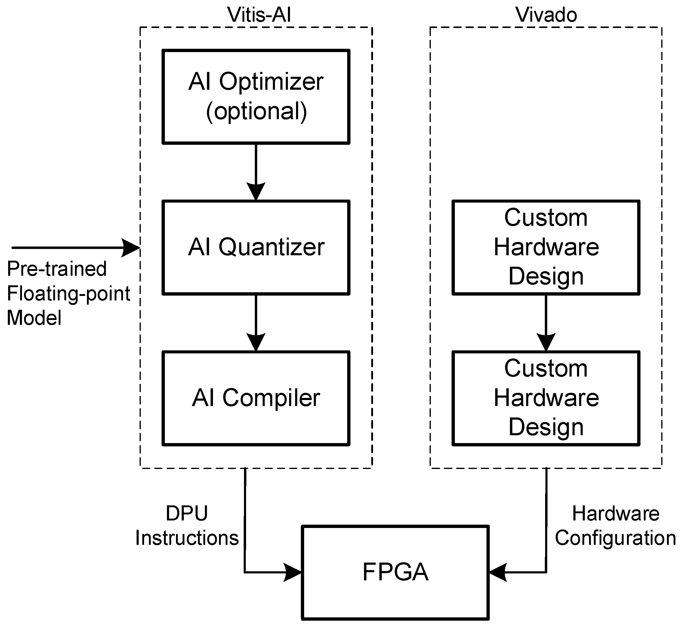
Vitis-AI integration: the integration of the dual-model inference with Vitis-AI. It automatically quantizes the solutions, compiles both models, and generates the runtime application;
3.
Design space exploration with ResNet: a systematic design space exploration of ResNet models by changing the repetition pattern of layers and the number of filters and resizing the input;
4.
System for skin cancer classification: a low-cost implementation of a system for skin cancer classification with a high accuracy.
The paper is organized as follows. Section 2 introduces the background and related work. Section 3 describes the dual-model design. Section 4 presents the results of the proposed system for skin cancer classification. Finally, Section 5 concludes the work.

2. Background and Related Work

2.1. Convolutional Neural Networks

A convolutional neural network (CNN) is a type of deep neural network used to analyze images. It has been applied successfully for image classification, image segmentation and object detection.
The main layer of a CNN is the convolutional layer. Given a set of input maps, the convolutional layer runs the convolution of several kernels of weights of size ( n o u t , i n z , k x y , k x y ) and a bias vector of size ( 1 , n o u t ) , where n o u t is the number of different filters, i n z is the depth of each filter, equal to the depth of the input image, and k x y is the size of the filter.
Each convolution between one kernel and the input maps generates an output map. After running the convolution with multiple kernels, the result is a 3D map of size ( n o u t , n y i n k x y + 1 , n x i n k x y + 1 ).
The behavior of each convolutional layer can be modified by two parameters: the stride and the padding. The stride determines the sliding size of the convolution; that is, the number of input pixels that each kernel slides over the map. In a normal convolution, where the filter slides through all input pixels, the stride is one. The stride is used to reduce the size of output maps relative to the size of the input map. Padding is used to preserve the size of the output map. One form of padding adds zeros at the border of the image.
Convolutional layers are used to extract features of an image. These features are then forwarded, for example, to a classifier to determine the class that the image belongs to in image classification problems. This classifier is usually implemented with a dense layer that determines the matrix multiplication between a matrix of weights, w, of size n i n , n o u t ), and the input map flattened to a vector of size 1 × n i n followed by an addition with a bias vector, b, with size (1, n o u t ). Its output function is A ( x . w + b ) , where A ( · ) is an activation function.
Equation (1) illustrates the multiply and accumulate operation required to calculate the n o u t outputs.
o u t j = i = 1 n i n x i · w i j + b j , o u t R n o u t
An important operation of deep neural networks is batch normalization [12], a method used to accelerate the training of the neural network model. It normalizes the layer inputs to a mean of 0 and variance of 1, and then scales and shifts the normalized inputs with learnable variables, γ and β .
During training, the training dataset is partitioned into batches. Batch normalization estimates a vector of means, μ R N , and a vector of variances, σ 2 R N , for each channel of the input image for each batch. The input shape will be ( M , C , Y , X ) , where M is the batch size and C is the number of X × Y planes.
First, as seen in Equation (2), where I represents the inputs, X × Y values are averaged per channel, resulting in an I ¯ , shaped as ( M , C ) . Then, the mean and variance values are calculated using Equations (3).
I ¯ ( m , c ) = 1 X . Y i = 1 Y j = 1 X I ( m , c , i , j )
μ ( c ) = 1 M i = 1 M I ¯ ( i , c ) σ 2 ( c ) = 1 M i = 1 M ( I ¯ ( i , c ) μ ( c ) ) 2
The mean and variance determined during training are used to normalize, scale and shift the inputs according to Equation (4), where γ and β are the variables learned during the training process and ϵ is a small constant value, commonly 10 5 , used for numerical stability [12].
I ^ = I μ σ 2 + ϵ I B N = γ · I ^ + β
Another common layer is the pooling layer that is used to downsample the input maps, reducing the size of the next input channels, with the same effect of the stride. Each window of a set elements of an input channel is replaced by the maximum (maxpooling) or the mean (average pooling) of all elements of the window.

2.2. Mapping CNNs on FPGAs

Several custom designed FPGA accelerators have already been proposed in the past using hardware description languages with very efficient core units. In [13], a CNN accelerator with an average performance of 400 GFLOPS was implemented in a low-density ZYNQ7020 FPGA. These handwritten hardware accelerators are very efficient in terms of performance and energy. However, the design of hardware accelerators using hardware description languages to run a deep learning model is a time-consuming task and difficult to redesign for other network models.
To avoid these long design times, designers started using high-level synthesis (HLS), which allows for the generation of hardware descriptions from the high-level specification of the algorithm in a programming language, like C, C++, OpenCL. Examples include the Xilinx Vivado HLS and the Intel FPGA OpenCL SDK.
Convolutional neural networks are well-defined structures with well-defined configurable layers. This regularity permits the development of domain-specific tools to map CNN on FPGA and the exploration of the design space.
The framework DNNWEAVER [14] automatically generates a Verilog description of an accelerator given a neural model and a target FPGA. The model is specified in Caffe [15] and the Verilog description uses hand-optimized templates. The framework includes an optimization tool to reorganize and batch the model operations to improve the utilization of internal resources of the FPGA.
fpgaConvNet [16] is another framework that automatically maps CNNs onto FPGAs. The tool receives a high-level description model in a custom representation and maps the layers in a streaming architecture with one processing unit per layer. It considers the most common type of layers, like convolutional, dense and pooling, and accepts application constraints, including throughput and latency. DeepBurning [17] follows a similar structure but, instead of a fixed schedule generated at compile time, like in fpgaConvNet, it requires control logic to dynamically schedule the operations.
FINN [18] was designed by Xilinx and supports the automatic mapping of neural models onto ZYNQ SoC FPGAs. The tool generates a streaming architecture in HLS and is particularly efficient for the design of low-quantization network models. The computing resources per layer can be customized to specific throughput requirements of the designer.
ALAMO [19] is a compiler that produces a configurable accelerator for the sequential implementation of layers in both FPGAs and application-specific integrated circuits (ASICs). The compiler automatically integrates computing primitives that accelerate the operations of deep neural models. It also optimizes the throughput for a given resource constraint.
HLS4ml [20] is an open-source software–hardware workflow used to automatically implement DNNs in FPGA or ASIC. The flow includes optimization techniques, like quantization and pruning, whose outcomes are supported by the automatic mapping on the target technology. The last version extends the tool to consider low-power implementations and a better reusability of the hardware. The designer controls the type of implementation to be generated, parallel or serial, and different precisions of the model are allowed. The performance, latency and resource utilization are the metrics considered in the design of the accelerator.
Vitis-AI (https://www.xilinx.com/products/design-tools/vitis/vitis-ai.html, accessed on 22 January 2023) is a development platform for Xilinx devices used to generate an accelerator for the inference of deep neural network models. It supports models specified in Pytorch, TensorFlow and Caffe. The approach considers a specialized configurable hardware core that supports the sequential execution of the most common layers. A set of custom instructions are used to dynamically configure the core to fit the specific needs of each layer. For this purpose, Vitis-AI has a compiler tool that transforms a neural network inference into a sequence of instructions. The communication between the core and the software is headed by a run-time application.
In this work, the objective is to design a low-area architecture. Therefore, streaming-like solutions are not an option since they occupy too much area and memory. Instead, a single configurable accelerator should be used. In addition, the solution should be flexible enough to allow for the execution of different models. Considering this, the Vitis-AI platform was adopted due to its flexibility and ease of utilization, the possibility to design different architectures with different performance–area ratios based on a single configurable accelerator and its support for Pytorch, the training framework adopted.

2.3. Skin Cancer Detection Using Deep Learning

The most common type of cancer is skin cancer, and it is spreading [21]. Detecting skin cancer at an early stage increases the survival rate to around 97% [22]. The medical procedure for skin cancer detection is time-consuming and aggressive to the patient when lesions must be biopsied [21].
Recently, AI-based algorithms have brought significant contributions to medical diagnosis; in particular, those based on medical imaging. Recent techniques, such as dermoscopy, have improved the visualization of lesions, improving the accuracy with which dermatological diagnosis are made. Many applications based on deep learning are already used to detect breast cancer, lung cancer, skin lesions, etc.
A dermatologist follows a sequence of steps to diagnose skin cancer, from direct observation to a biopsy. However, this is a time-consuming process that compromises an early cancer detection [23].
Image classification with deep learning has therefore been applied to help the medical diagnosis. Popescu et al. [24] considered several CNN-based models to classify images in the HAM10000 dataset. Each individual output is combined into a decision fusion module. The results report an accuracy of 86.71%, 3% higher than the best individual model. The better accuracy has a high cost in terms of computing resources and energy and, therefore, is not appropriate for portable devices. Srinivasu et al. [25] proposed a deep-learning model as a combination of MobileNet and a long short-term memory model. The combined model achieved an accuracy of 85% on the HAM10000 dataset.
In [26], Khan et al. considered a mask recurrent neural network and a pyramid neural network to classify images from the HAM10000 dataset, with a precision of 87%. The work was improved to an accuracy of 90.7% [27] using a color-controlled histogram, a new saliency segmentation technique with a CNN. Finally, a kernel extreme learning machine classifier was used.
Karl and Enrique [28] also considered the skin cancer identification problem. The solution applies transfer learning to a CNN, obtaining a validation accuracy of 87.8%. Saket et al. [29] used the MobileNet model and transfer learning to classify HAM10000 images, with a final accuracy of 83.1%. Ameri et al. [30] and Khushi et al. [31] also considered deep learning and transfer learning for skin cancer classification. The second only distinguished between melanoma and non-melanoma images, instead of classifying among the seven possible classes of HAM10000.
In general, deep neural models and transfer learning are used to train models for skin cancer classification. Most solutions have an accuracy of around 87%, with lower-complexity models such as MobileNet achieving 85% and more complex models achieving almost 91%.
In this work, the family of ResNet models was considered and explored in order to implement the classification problem with incremental inference. However, other models could be considered, such as MobileNet. The proposed incremental inference can also be run with different models. For example, a MobileNet could be used for the lowest complexity model and a ResNet for the more accurate model.

2.4. Vitis AI

The Vitis AI development environment includes optimized IP cores, tools, libraries and pre-trained models. It is designed for a high design efficiency and ease of use in order to unleash the full potential of AI acceleration on Xilinx FPGAs. With Vitis AI, the network intended for implementation on the FPGA can be quantized and pruned.
Vitis-AI compiles the model to be implemented in a programmable engine (DPU—deep learning processing unit) dedicated to the acceleration of the inference of a neural network (see Figure 1).
Vitis-AI receives a pre-trained model and applies quantization (8-bit fixed-point). Pruning can also be applied optionally. The quantized model is then compiled to the target DPU architecture to generate an executable to run in the DPU. The hardware/software system architecture with the DPU can be designed in the Vivado or Vitis frameworks.
Several parameters of the DPU can be configured to meet the performance requirements of different applications. This reduces the space occupied by the FPGA as much as possible. The set of parameters includes:
  • Number of cores: A DPU instance can include up to four different cores. The greater the number of cores, the greater the implementation performs, but the amount of resources used increase accordingly;
  • Architecture: Different types of architectures based on the level of parallelism. A number of designs are available based on the number of operations that they can perform per clock cycle: B512, B800, B1024, B1152, B1600, B2304, B3136 and B4096. This value is directly correlated with the level of parallelism. In particular, the higher the parallelism, the higher the number of executable operations and necessary resources;
  • RAM usage: To increase performance, on-chip RAM memory is used to store weights, bias, and intermediate results. When instantiating the DPU module, it is possible to choose the amount of RAM that will be reserved for the CNN. This can be done by selecting between the high RAM usage and low RAM usage option;
  • Channel augmentation: An approach that exploits the fact that, in some models, the number of input channels is lower than the parallelism between the channels in the architecture. By enabling this option when this condition is met, the performance can be improved at the cost of using more resources;
  • Depth-wise convolution: With standard convolution, each input channel needs to perform some operations with one specific kernel. Then, all of the results of all of the channels are combined to obtain the final result. When depth-wise convolution is enabled, the convolution operation is split into two parts: depth-wise and point-wise. The former allows for processing the input channels in parallel, whereas the latter performs convolution with a 1 × 1 kernel. This combines the results of the previous step to obtain the final value. With this approach, the parallelism of the depth-wise convolution is lower than that of pixel parallelism, allowing for more than one activation map to be evaluated per clock cycle.
DPU implementations can be customized to find the best balance between resources and performance by combining the above features. As soon as the configuration process is complete, it is necessary to save the enabled options so that the compiler can correctly select the instructions. This step is automatically performed after the synthesis of the DPU.

2.5. Embedded Systems for Portable Health Devices

Portable health devices are changing people’s lives by providing a monitoring and prevention tool [32]. The recent advances in deep learning and its applicability in the health domain have changed these health devices from passive, monitoring solutions to smart active real-time analysis of many health aspects. Running complex and accurate models on embedded and portable systems is challenging. In addition, many of these solutions must be customized to the users’ needs. Therefore, it is important to provide accessible tools and devices that allow for the deployment of smart custom health devices.
The system proposed in this paper is an effort made toward this type of solutions. It proposes a solution to increase the classification throughput while keeping the high accuracy, and a user-friendly design tool to design and map the dual model in an FPGA for a low-cost, low-power custom embedded solution.

3. Dual-Model Design

The objective of using two models incrementally during inference is to have a system with a performance and energy consumption close to that of the smaller model and an accuracy close to that of the larger model. The pair of models determines the performance, energy and accuracy of the final system.
An important component of the dual-model inference is the confidence predictor, which determines the confidence of image classification. An image classified with low confidence needs to be classified again with the more accurate model. The confidence predictor requires a function to determine the confidence of a classification and a threshold that establishes the border between confident and non-confident.
Some works consider the softmax output probabilities and calculate the difference between the highest probability and the accumulation of a subset of the remaining probabilities to assess the confidence of the model outcome [6]. This metric, however, is relatively weak in determining the robustness of the model. Instead, entropy is considered to be a more robust metric [33]. Both methods were analyzed and tested in the context of this work and the entropy metric provided better results. In addition, calculating the entropy for a small set of classes is quick.
In this work, the confidence of a classification, c o n f t o p 1 , was calculated as the absolute value of the entropy of the probability output array of the final layer as follows:
C o n f t o p 1 = | i p i × l o g ( p i ) |
where p i is the probability associated with a class. The classification of an image is considered confident if C o n f t o p 1 t h e n t r o p y , where t h e n t r o p y is the entropy threshold of the confidence. The threshold determines the ratio between the accuracy and inference runtime. As the threshold is reduced, the number of images that need to be classified with the more accurate model increases, which increases the accuracy of the dual model. However, since the more accurate and slower model is executed more times, the average runtime of the dual-model inference increases.
Given a pair of models and an accuracy tolerance, Tacy (relative to the accuracy of the most accurate model), a tool was developed to find the confidence threshold with an accuracy within the accuracy error and a lower inference runtime. The final dual model should be faster and within the accuracy tolerance.
The tool developed in Python receives two trained models with different accuracy levels and the accuracy range. It then finds the fastest multi-model configuration with an accuracy within the accuracy range, according to the design flow illustrated in Figure 2.
The design flow has the following steps:
1.
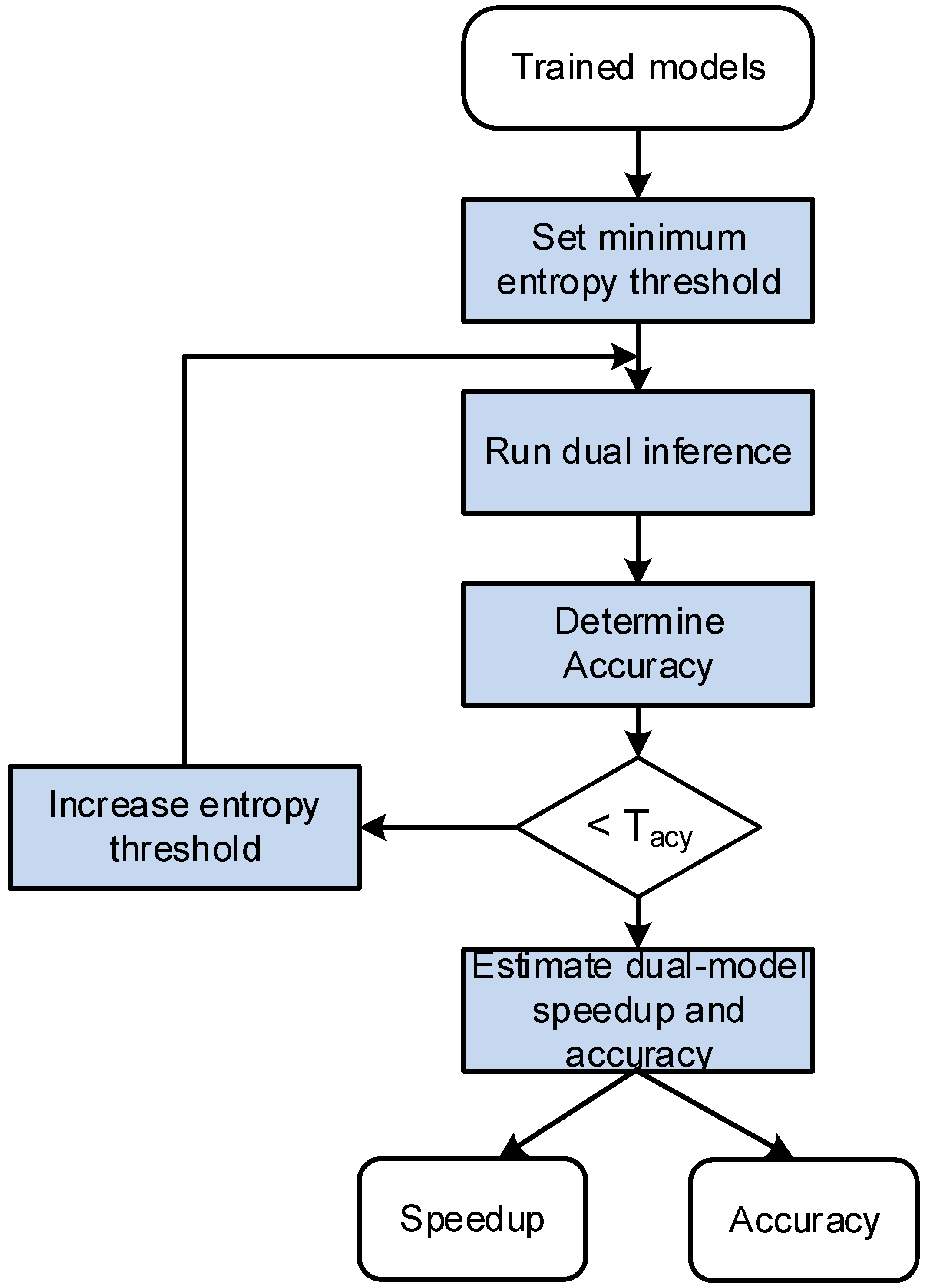
Trained Models—The models are previously trained;
2.
Set minimum entropy threshold—The minimum initial entropy threshold and the entropy increment are defined. As explained above, this threshold is used by the confidence predictor. In this work, both parameters were initialized at 0.1;
3.
Run dual inference—The dual-model inference is run with the entropy threshold set previously. The task runs the inference with the smaller model and the training dataset. For each sample, it finds the entropy. If the entropy is higher than the entropy threshold, it runs the second model. This process allows us to determine the accuracy of the dual model;
4.
Determine accuracy—The accuracy corresponds to the number of samples correctly classified by the first model and by the second model, whenever it runs, divided by the total number of samples. If the accuracy is within the accuracy tolerance, the entropy threshold is increased by 0.1 and the process repeats;
5.
Estimate speedup and accuracy—The speedup is estimated as follows:
M 2 O P S M 1 O P S + M 2 O P S × S 2
where M X O P S is the number of operations of the model, and S X is the percentage of inputs executed by model X. The accuracy is given by the previous step.

4. Results

The dual-model design flow was integrated with the Vitis-AI platform. The deep learning framework used was Pytorch, with all code developed in Python. The tool was then applied to the design of an FPGA-based system for skin cancer classification. The models were trained in an NVIDIA RTX2080Ti GPU with 12 GB of memory, and the system was implemented in a ZYNQ UltraScale+ MPSoC ZCU104 evaluation kit with a ZU7EV device.

4.1. HAM10000 Dataset

The training of neural networks for the automated diagnosis of pigmented skin lesions is hampered by the small size and lack of diversity of available dataset of dermatoscopic images. It was decided to use the HAM10000 dataset [34] as it consists of a collection of dermatoscopic images from a variety of populations, acquired and stored through various methods. Upon completion, the final dataset consists of 10,015 dermatoscopic images, which can be used for academic machine learning experiments. In addition, it is the dataset used in most of the previous works about this subject.
In more than half of the cases, histopathology confirms the diagnosis, and, for the remainder, follow-up examination, expert consensus or in vivo confocal microscopy was used [34].
Additionally, the dataset includes a metadata file where each case is identified by a diagnosis representation, which includes all of the important classifications in pigmented lesions and correlates them with the dataset images. The seven categories and their corresponding abbreviations that are evaluated by our network are listed in Table 1.
There is also an unbalanced sample size across the classes, with 67% of the samples coming from the “melanocytic nevi” or “nv” class, followed by 11% for the “melanoma” class and the remaining five classes accounting for the remaining 22%. Asymmetry occurs as a result of how common some of these diseases are, as well as how different populations are affected by them. “Benign keratosis-like lesions” are a good example, and are more prevalent among older people.

4.2. Single Network Model

Several known CNN models can be utilized to classify skin cancer lesions. The most adequate for the problem at hand depends on the tradeoffs between the classification accuracy, complexity and facility to be quantized. Three variants of ResNet (ResNet18, ResNet50 and ResNet101) were considered for this purpose. The metrics used to compare the models were accuracy, precision, recall, and F1-score. These metrics are defined as follows:
A c c u r a c y = T P + T N T P + F P + F N + T N
P r e c i s i o n = T P T P + F P
R e c a l l = T P T P + F N
F 1 - s c o r e = 2 × R e c a l l × P r e c i s i o n R e c a l l + P r e c i s i o n
where
1.
True Positive (TP): Correctly predicted positive values;
2.
True Negative (TN): Correctly predicted negative values. Both predicted and actual values are negative;
3.
False Positive (FP): The predicted value is positive but the correct value is negative;
4.
False Negative (FN): The predicted value is negative but the correct value is positive.
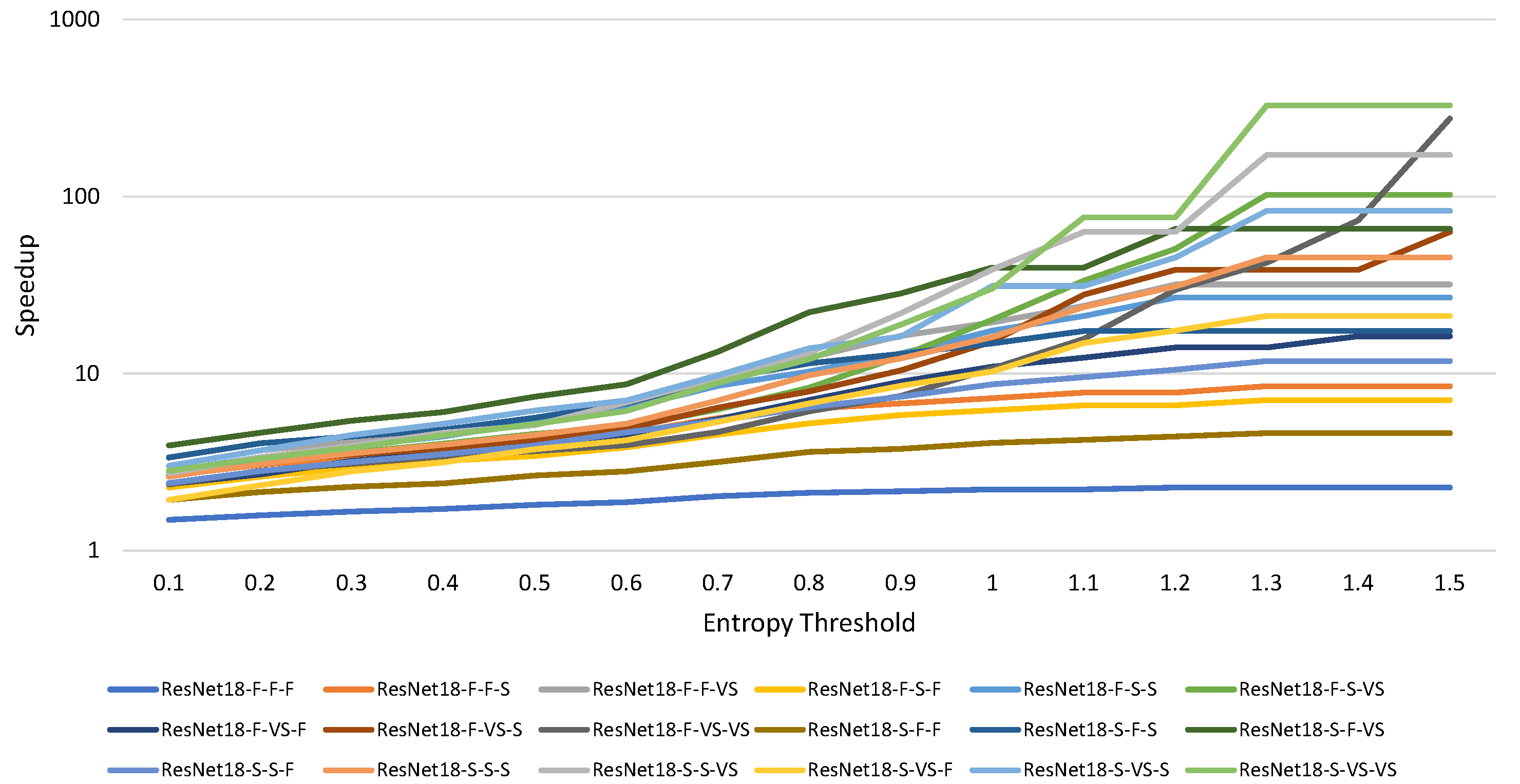
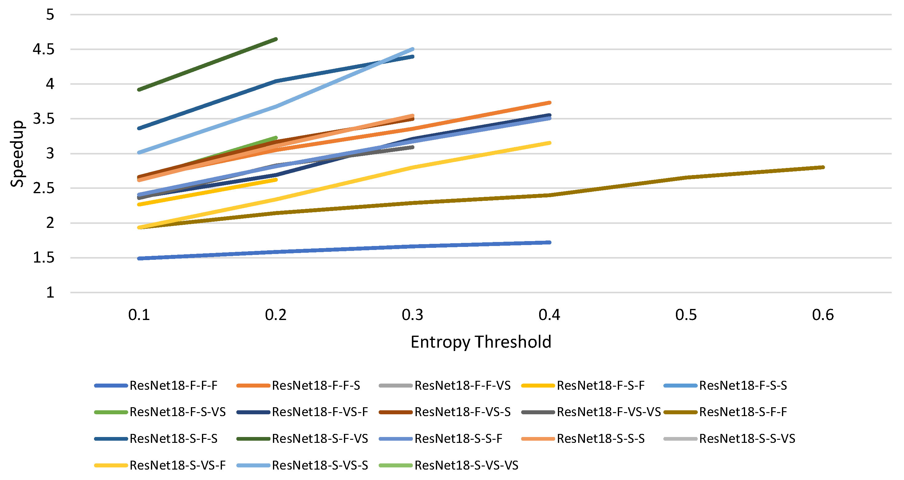
Accuracy is the most intuitive measure and is simply a ratio of correctly predicted observations to total observations. This metric is enough for symmetric datasets where values of false positives and false negatives are almost the same. The precision determines how much of the images identified as positive detections are correct. Recall determines how many positive cases were detected out of all of the positive cases. Finally, the F1-score is useful when there is an uneven class distribution.
The four network models were trained for 50 epochs with the HAM10000 dataset and the results of the four metrics were determined (see results in Table 2). In the first experiment, all images used in the network were resized to 224 × 224 .
The table includes the number of parameters ( P a r a m ) and the number of floating-point operations (FLOPS) of a single inference. As can be seen from the results, ResNet18 is close to the results of ResNet50, using only half of the parameters and less than half of the operations.
Since the results obtained with the models are close to each other, smaller variants of ResNet18 model were considered. These are identified as ResNet18-X-Y-M:
1.
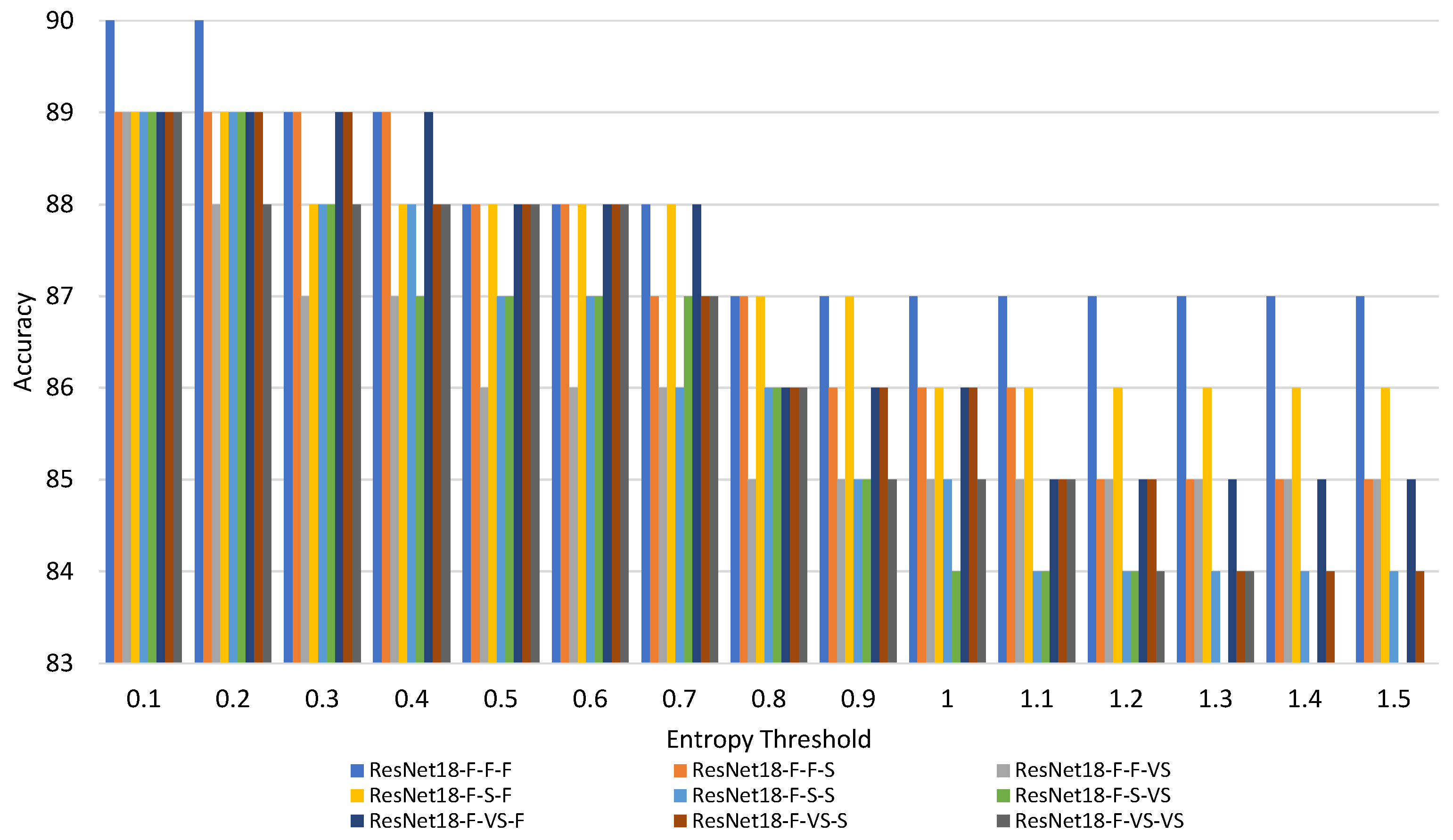
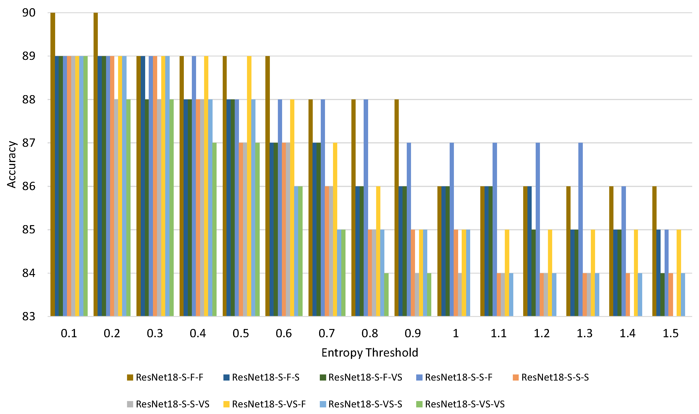
X: Indicates the repetition pattern of the basic block. Two repetition patterns are considered: (F) the original ResNet18 repetition pattern, [2, 2, 2, 2], and (S) a reduced repetition pattern, [1, 1, 1, 1];
2.
Y: Indicates the number of filters. Three different variations are considered: the original (F), one with half of the filters in all layers (S) and another with a quarter of the filters in all layers (VS);
3.
M: Indicates the size of the images. Three different resizes are considered: 224 × 224 (F), 112 × 112 (S) and 56 × 56 (VS).
All variants were trained and evaluated with the HAM10000 dataset. The dataset was divided into two parts: 80% of the images for training and 20% for evaluation. The models were trained for 50 epochs with a batch size of 32 using the Adam optimization algorithm and a cross entropy loss function. The learning rate was initially set to 0.001 and a cosine annealing learning rate adjustment strategy was used. The results of the four metrics were determined (see results in Table 3).
As can be seen from the results in the table, there is a small accuracy penalty (up to 5%) for the less accurate model compared to ResNet50 due to the large reduction in the number of parameters and operations of the model. For example, ResNet18-S-VS-VS needs 73 × fewer parameters and around a 5 × lower number of operations compared to ResNet50. These results are very important for the dual model since there is a notable reduction in the complexity of the smaller model compared to the larger one, with only a 5% reduction in accuracy.

4.3. Dual Model

After training all variants of ResNet, the design flow for the dual model design was applied, considering all variants as the smaller model and ResNet50 as the larger model. The accuracy and the theoretical speedup were determined for all cases (see Figure 3, Figure 4 and Figure 5).
As expected, the accuracy decreases as we increase the entropy threshold, since the confidence of the smaller model increases, which consequently increases the number of images wrongly classified. On the other side, the speedup increases since fewer images are sent for reclassification with the larger model.
Considering the accuracy, it is interesting to observe that the dual model is able to improve the accuracy of the ResNet50 model and still achieve some speedup. For example the combination of ResNet18-F-F-F with ResNet50 achieves an accuracy of 90% with a speedup of 1.5. To further understand why this happens, a detailed analysis of the outcomes of both models was carried out. This could only happen if the lower-accuracy model was correctly classifying some instances that were incorrectly classified by the higher-accuracy model. This fact was observed, and it also slightly compensates for some false positives. This observation is also valid for other entropy thresholds but, as we increase this threshold, the false positives also increase, and the peak accuracy is no longer observed.
High speedups are possible using the very small models. However, these models lose some accuracy. In fairness, in the comparison, only those dual models with the same accuracy as or a higher accuracy than model ResNet50 were considered (see Figure 6).
The highest speedup (×4.7) is achieved with ResNet-S-F-VS, with an accuracy of 89%. A similar analysis can be performed for any accuracy. For example, with an accuracy of 88%, architecture ResNet18-S-F-VS has a speedup of ×7.4 compared to ResNet50.

4.4. Performance of the Accelerator

The models were quantized and mapped in a ZYNQ UltraScale+ MPSoC ZCU104 platform using Vitis-AI.
The first implementation was with a single model without model reduction, ResNet18-F-F-F. The system was executed with different DPU configurations running at 300 MHz. The area occupation and the throughput (frames per second—FPS) are reported in Table 4 for different DPU configurations. The DPU reference indicates the number of operations per second (OPSs).
As expected, smaller DPUs require fewer resources but are also slower. The throughput reduces proportionally with the number of parallel operations.
All dual models were tested in software to measure the accuracy and to later be compared with the onboard results. The results show a small range of results between 86.4% and 87.1%, with the mean being 86.8%. Therefore, the accuracy degradation caused by quantization is very small.
Considering that the application is to be run in an embedded system, the following experiments considered only the hardware solution with a B512 DPU.
All dual models using the ResNet50 as the more accurate model were generated. Dual models with the same accuracy as or higher accuracy than ResNet50 after quantization were considered to run and test on the board. All dual models were compiled using the developed flow and run on the board. A script was written to automatically run all dual models serially in the DPU and to save the results. The synthesis tool reports a power ranging from 3 to 4 W for the whole FPGA. An extra 1 W was considered for the access to the external memory of the board. Thus, a total maximum of 5 W is reported for the system. The comparison metrics were the accuracy, the throughput and the energy per frame (see Table 5).
From the results, it is possible to identify two solutions with an accuracy higher than ResNet50 and a higher performance. The best dual model, with an accuracy of 88%, includes the architecture ResNet18-S-F-F. With an accuracy of 87%, the best dual model (ResNet18-S–F-VS/ResNet50) achieves a performance of 13.5 FPS (speedup of × 4.3 ).
As far as we know, there are no previous FPGA implementations for the classification of the HAM10000 dataset. There are a few FPGA implementations for skin cancer identification, with only two classes (cancer/no cancer) using an SVM classifier [35].

5. Conclusions and Future Work

This paper describes the design of a low-cost system for skin cancer classification implemented in an FPGA. The deep learning model considers two models with different accuracies and complexities. The more accurate model only runs in the case of a low confident classification of the less complex model.
The models were quantized and mapped to the FPGA using a Vitis-AI design flow. The system achieves 13.5 FPS with an accuracy of 87% with minimal resources, and 6.2 FPS with an accuracy of 88%. The proposed solution is accurate and can run in low-density devices with an acceptable throughput. It helps in achieving solutions with the same accuracy as highly accurate models with a higher throughput or a smaller device.
Only networks within the ResNet family were considered in this work. However, other models, like MobileNet, can be considered. The dual-model technique is now being applied to an object detection problem.

Author Contributions

Conceptualization, P.F.D. and M.P.V.; methodology, P.F.D. and M.P.V.; software, P.F.D.; validation, P.F.D. and M.P.V.; formal analysis, P.F.D.; investigation, P.F.D. and M.P.V.; resources, P.F.D. and M.P.V.; data curation, P.F.D.; writing—original draft preparation, P.F.D.; writing—review and editing, M.P.V.; visualization, P.F.D. and M.P.V.; supervision, M.P.V.; project administration, M.P.V.; funding acquisition, M.P.V. All authors have read and agreed to the published version of the manuscript.

Funding

This work was supported by national funds through Fundação para a Ciência e a Tecnologia (FCT) with reference UIDB/50021/2020 and IPL/2022/eS2ST_ISEL through Instituto Politécnico de Lisboa.

Institutional Review Board Statement

Not applicable.

Informed Consent Statement

Not applicable.

Conflicts of Interest

The authors declare no conflict of interest.

References

  1. Egger, J.; Gsaxner, C.; Pepe, A.; Pomykala, K.L.; Jonske, F.; Kurz, M.; Li, J.; Kleesiek, J. Medical deep learning—A systematic meta-review. Comput. Methods Programs Biomed. 2022, 221, 106874. [Google Scholar] [CrossRef] [PubMed]
  2. Gholami, A.; Kim, S.; Dong, Z.; Yao, Z.; Mahoney, M.W.; Keutzer, K. A Survey of Quantization Methods for Efficient Neural Network Inference. arXiv 2021, arXiv:2103.13630. [Google Scholar]
  3. Alqahtani, A.; Xie, X.; Jones, M.W. Literature Review of Deep Network Compression. Informatics 2021, 8, 77. [Google Scholar] [CrossRef]
  4. Wu, C.; Wang, M.; Chu, X.; Wang, K.; He, L. Low-Precision Floating-Point Arithmetic for High-Performance FPGA-Based CNN Acceleration. ACM Trans. Reconfigurable Technol. Syst. 2021, 15, 1–21. [Google Scholar] [CrossRef]
  5. Viola, P.; Jones, M.J. Robust Real-Time Face Detection. Int. J. Comput. Vis. 2004, 57, 137–154. [Google Scholar] [CrossRef]
  6. Kouris, A.; Venieris, S.I.; Bouganis, C. CascadeCNN: Pushing the Performance Limits of Quantisation in Convolutional Neural Networks. In Proceedings of the 2018 28th International Conference on Field Programmable Logic and Applications (FPL), Dublin, Ireland, 26–30 August 2018; pp. 155–1557. [Google Scholar] [CrossRef] [Green Version]
  7. De Sousa, A.L.; Véstias, M.P.; Neto, H.C. Multi-Model Inference Accelerator for Binary Convolutional Neural Networks. Electronics 2022, 11, 3966. [Google Scholar] [CrossRef]
  8. Guo, P.; Ma, H.; Chen, R.; Li, P.; Xie, S.; Wang, D. FBNA: A Fully Binarized Neural Network Accelerator. In Proceedings of the 2018 28th International Conference on Field Programmable Logic and Applications (FPL), Dublin, Ireland, 27–31 August 2018; pp. 51–513. [Google Scholar] [CrossRef]
  9. Véstias, M.P. A Survey of Convolutional Neural Networks on Edge with Reconfigurable Computing. Algorithms 2019, 12, 154. [Google Scholar] [CrossRef] [Green Version]
  10. Venieris, S.; Kouris, A.; Bouganis, C. Toolflows for Mapping Convolutional Neural Networks on FPGAs: A Survey and Future Directions. ACM Comput. Surv. 2018, 51, 1–39. [Google Scholar] [CrossRef] [Green Version]
  11. He, K.; Zhang, X.; Ren, S.; Sun, J. Deep Residual Learning for Image Recognition. In Proceedings of the 2016 IEEE Conference on Computer Vision and Pattern Recognition (CVPR), Las Vegas, NV, USA, 27–30 June 2016; pp. 770–778. [Google Scholar] [CrossRef] [Green Version]
  12. Ioffe, S.; Szegedy, C. Batch Normalization: Accelerating Deep Network Training by Reducing Internal Covariate Shift. arXiv 2015, arXiv:1502.03167. [Google Scholar]
  13. Véstias, M.P.; Duarte, R.P.; de Sousa, J.T.; Neto, H.C. A fast and scalable architecture to run convolutional neural networks in low density FPGAs. Microprocess. Microsyst. 2020, 77, 103136. [Google Scholar] [CrossRef]
  14. Sharma, H.; Park, J.; Mahajan, D.; Amaro, E.; Kim, J.K.; Shao, C.; Mishra, A.; Esmaeilzadeh, H. From high-level deep neural models to FPGAs. In Proceedings of the Microarchitecture (MICRO), 2016 49th Annual IEEE/ACM International Symposium on Microarchitecture, Taipei, Taiwan, 15–19 October 2016; IEEE: Piscataway, NJ, USA, 2016; pp. 1–12. [Google Scholar]
  15. Jia, Y.; Shelhamer, E.; Donahue, J.; Karayev, S.; Long, J.; Girshick, R.; Guadarrama, S.; Darrell, T. Caffe: Convolutional Architecture for Fast Feature Embedding. arXiv 2014, arXiv:1408.5093. [Google Scholar]
  16. Venieris, S.I.; Bouganis, C.S. fpgaConvNet: A Framework for Mapping Convolutional Neural Networks on FPGAs. In Proceedings of the 2016 IEEE 24th Annual International Symposium on Field-Programmable Custom Computing Machines (FCCM), Washington, DC, USA, 1–3 May 2016; pp. 40–47. [Google Scholar] [CrossRef] [Green Version]
  17. Wang, Y.; Xu, J.; Han, Y.; Li, H.; Li, X. DeepBurning: Automatic generation of FPGA-based learning accelerators for the Neural Network family. In Proceedings of the 2016 53nd ACM/EDAC/IEEE Design Automation Conference (DAC), Austin, TX, USA, 5–9 June 2016; pp. 1–6. [Google Scholar] [CrossRef]
  18. Blott, M.; Preußer, T.B.; Fraser, N.J.; Gambardella, G.; O’Brien, K.; Umuroglu, Y. FINN-R: An End-to-End Deep-Learning Framework for Fast Exploration of Quantized Neural Networks. arXiv 2018, arXiv:1809.04570. [Google Scholar] [CrossRef]
  19. Wilson, Z.T.; Sahinidis, N.V. The ALAMO approach to machine learning. arXiv 2017, arXiv:1705.10918. [Google Scholar] [CrossRef] [Green Version]
  20. Vloncar; Summers, S.; Duarte, J.; Tran, N.; Kreis, B.; Jngadiub; Ghielmetti, N.; Hoang, D.; Kreinar, E.J.; Lin, K.; et al. Fastmachinelearning/hls4ml: Coris (v0.6.0). arXiv 2021, arXiv:1804.06913. [Google Scholar]
  21. Tavakolpour, S.; Daneshpazhooh, M.; Mahmoudi, H. Skin Cancer: Genetics, Immunology, Treatments, and Psychological Care. In Cancer Genetics and Psychotherapy; Springer International Publishing: Cham, Switzerland, 2017; pp. 851–934. [Google Scholar] [CrossRef]
  22. Niino, M.; Matsuda, T. Age-specific skin cancer incidence rate in the world. Jpn. J. Clin. Oncol. 2021, 51, 848–849. [Google Scholar] [CrossRef]
  23. Wolner, Z.J.; Yélamos, O.; Liopyris, K.; Rogers, T.; Marchetti, M.A.; Marghoob, A.A. Enhancing Skin Cancer Diagnosis with Dermoscopy. Dermatol. Clin. 2017, 35, 417–437. [Google Scholar] [CrossRef]
  24. Popescu, D.; El-khatib, M.; Ichim, L. Skin Lesion Classification Using Collective Intelligence of Multiple Neural Networks. Sensors 2022, 22, 4399. [Google Scholar] [CrossRef]
  25. Srinivasu, P.N.; SivaSai, J.G.; Ijaz, M.F.; Bhoi, A.K.; Kim, W.; Kang, J.J. Classification of Skin Disease Using Deep Learning Neural Networks with MobileNet V2 and LSTM. Sensors 2021, 21, 2852. [Google Scholar] [CrossRef]
  26. Khan, M.A.; Zhang, Y.D.; Sharif, M.; Akram, T. Pixels to Classes: Intelligent Learning Framework for Multiclass Skin Lesion Localization and Classification. Comput. Electr. Eng. 2021, 90, 106956. [Google Scholar] [CrossRef]
  27. Khan, M.A.; Sharif, M.; Akram, T.; Damaševičius, R.; Maskeliūnas, R. Skin Lesion Segmentation and Multiclass Classification Using Deep Learning Features and Improved Moth Flame Optimization. Diagnostics 2021, 11, 811. [Google Scholar] [CrossRef]
  28. Thurnhofer-Hemsi, K.; Domínguez, E. A Convolutional Neural Network Framework for Accurate Skin Cancer Detection. Neural Process. Lett. 2021, 53, 3073–3093. [Google Scholar] [CrossRef]
  29. Chaturvedi, S.S.; Gupta, K.; Prasad, P.S. Skin Lesion Analyser: An Efficient Seven-Way Multi-class Skin Cancer Classification Using MobileNet. In Advances in Intelligent Systems and Computing; Springer: Singapore, 2020; pp. 165–176. [Google Scholar] [CrossRef]
  30. Ameri, A. A Deep Learning Approach to Skin Cancer Detection in Dermoscopy Images. J. Biomed. Phys. Eng. 2020, 10, 801–806. [Google Scholar] [CrossRef] [PubMed]
  31. Khushi, M.; Shaukat, K.; Alam, T.M.; Hameed, I.A.; Uddin, S.; Luo, S.; Yang, X.; Reyes, M.C. A Comparative Performance Analysis of Data Resampling Methods on Imbalance Medical Data. IEEE Access 2021, 9, 109960–109975. [Google Scholar] [CrossRef]
  32. Mukherjee, S.; Suleman, S.; Pilloton, R.; Narang, J.; Rani, K. State of the Art in Smart Portable, Wearable, Ingestible and Implantable Devices for Health Status Monitoring and Disease Management. Sensors 2022, 22, 4228. [Google Scholar] [CrossRef] [PubMed]
  33. Tornetta, G.N. Entropy Methods for the Confidence Assessment of Probabilistic Classification Models. Statistica 2021, 81, 383–398. [Google Scholar] [CrossRef]
  34. Tschandl, P. The HAM10000 Dataset, a Large Collection of Multi-Source Dermatoscopic Images of Common Pigmented Skin Lesions, Harvard Dataverse, V3; Medical University of Vienna: Vienna, Austria, 2018. [Google Scholar] [CrossRef]
  35. Afifi, S.; GholamHosseini, H.; Sinha, R. A system on chip for melanoma detection using FPGA-based SVM classifier. Microprocess. Microsyst. 2019, 65, 57–68. [Google Scholar] [CrossRef]
Figure 1. Project flow using Vitis-AI.
Futureinternet 15 00052 g001
Figure 2. Design flow used to find the best dual model.
Futureinternet 15 00052 g002
Figure 3. Accuracy of the dual model for different combinations of a small model with ResNet50. The small models in the graphic are all variants of ResNet18 described above restricted to the repetition pattern of the original ResNet18.
Futureinternet 15 00052 g003
Figure 4. Accuracy of the dual model for different combinations of a small model with ResNet50. The small models in the graphic are all variants of ResNet18 described above restricted to the reduced repetition pattern of ResNet18.
Futureinternet 15 00052 g004
Figure 5. Speedup of the dual model for different combinations of a small model with ResNet50.
Futureinternet 15 00052 g005
Figure 6. Speedup of the dual model for different combinations of a small model with ResNet50.
Futureinternet 15 00052 g006
Table 1. Image classes of HAM10000 dataset.
Lesion NameLesion Abreviation
Actinic keratoses and intraepithelial carcinomaakiec
basal cell carcinomabcc
benign keratosis-like lesionsbkl
dermatofibromadf
melanomamel
melanocytic nevinv
vascular lesionsvasc
Table 2. Training results for three variants of ResNet.
ModelParam ( × 10 6 )FLOPS ( × 10 9 )AccuracyPrecisionRecallF1-Score
ResNet1811.181.830.880.870.880.86
ResNet5023.54.130.890.880.880.87
ResNet10144.57.610.900.900.890.88
Table 3. Training results for the four network models.
ModelParam ( × 10 6 )MOPS ( × 10 9 )Accuracy
ResNet18-F-F-F11.181.830.88
ResNet18-F-F-S11.180.490.86
ResNet18-F-F-VS11.180.130.85
ResNet18-F-S-F2.820.580.84
ResNet18-F-S-S2.820.150.85
ResNet18-F-S-VS2.820.040.84
ResNet18-F-VS-F0.720.250.87
ResNet18-F-VS-S0.720.070.85
ResNet18-F-VS-VS0.720.020.84
ResNet18-S-F-F4.900.900.88
ResNet18-S-F-S4.900.240.86
ResNet18-S-F-VS4.900.060.87
ResNet18-S-S-F1.250.350.86
ResNet18-S-S-S1.250.090.85
ResNet18-S-S-VS1.250.020.84
ResNet18-S-VS-F0.330.200.86
ResNet18-S-VS-S0.330.050.86
ResNet18-S-VS-VS0.330.010.84
Table 4. Occupation of resources and throughput for different architectures of the DPU running the inference of ResNet18-F-F-F.
DPULUTFFDSPBRAMURAMFPS
B409654533999525282541220
B230446718723143041661121
B10243869651848144102151
B51233374395408070124
Table 5. Accuracy and performance of dual models running in the FPGA.
Param ( × 10 6 )Performance (FPS)Energy/Frame (J)
Model Acc = 88%Acc = 87%Acc = 87%
ResNet5023.53.11.61
ResNet18-F-F-F34.74.65.01.00
ResNet18-F-F-S34.710.80.46
ResNet18-F-F-VS34.78.80.57
ResNet18-F-S-F26.37.60.66
ResNet18-F-S-S26.39.80.51
ResNet18-F-S-VS26.39.40.53
ResNet18-F-VS-F24.210.30.49
ResNet18-F-VS-S24.210.10.50
ResNet18-F-VS-VS24.26.80.74
ResNet18-S-F-F28.46.28.10.62
ResNet18-S-F-S28.412.70.39
ResNet18-S-F-VS28.413.50.37
ResNet18-S-S-F24.810.20.49
ResNet18-S-S-S24.810.30.49
ResNet18-S-S-VS24.87.90.63
ResNet18-S-VS-F23.810.80.46
ResNet18-S-VS-S23.813.10.38
ResNet18-S-VS-VS23.88.20.61
Disclaimer/Publisher’s Note: The statements, opinions and data contained in all publications are solely those of the individual author(s) and contributor(s) and not of MDPI and/or the editor(s). MDPI and/or the editor(s) disclaim responsibility for any injury to people or property resulting from any ideas, methods, instructions or products referred to in the content.

