A Digital Twin Framework Embedded with POD and Neural Network for Flow Field Monitoring of Push-Plate Kiln

Abstract

The push-plate kiln is a kind of kiln equipment widely used in the oxygen-free sintering of high-temperature alloy materials. Its flow field monitoring has an important application value for the manufacturing industry. However, traditional simulation methods cannot meet the requirements of real-time applications due to the high computational cost and being time-consuming. The rapid development of artificial intelligence technology will empower the traditional manufacturing industry. In this paper, we propose a data-driven digital twin framework for real-time flow field prediction by combining the CFD modeling simulation, IoT, and deep learning technologies. The framework integrates geometric, rule, physical, and neural network models to achieve the real-time simulation of physical and twin objects. The proper orthogonal decomposition (POD) and multiscale convolutional neural network (MCNN) are innovatively embedded into the framework. The POD is used to map high-dimensional data to low-dimensional features, and the MCNN is used to construct models predicting low-dimensional features for fast flow field prediction. The effectiveness of the proposed model is verified by the push-plate kiln case. The results show that the digital twin can quickly predict multi-physics fields based on the perceptual data to achieve the real-time evaluation of the operating state of the push-plate kiln.

1. Introduction

By integrating advanced information technology, the Cyber-Physical System (CPS) builds a complex system of efficient coordination between the physical and information space, and realizes on-demand response, rapid iteration, and dynamic optimization of the system operation [1]. In recent years, the development of multi-physics solvers, the Internet of Things, big data, and artificial intelligence have enabled us to make digital twins (DT) of large-scale physical systems [2,3], using sensor and simulation data to solve problems, such as control, monitoring, and improved decision-making. These technologies have promoted the transformation of the manufacturing industry to digitalization and intelligence.

The push-plate kiln is a continuous heating and sintering equipment that arranges the required temperature to meet the product’s heat demand according to the sintered product’s process requirements. Its working process is a typical multidisciplinary coupling process involving the related theoretical knowledge, such as physics, mechanics, and heat transfer [4,5]. The state of its internal temperature field and pressure field has an important application value for the remote monitoring and real-time regulation of the production process. The failure of the kiln will lead to a huge loss of productivity and profits. However, the traditional manufacturing process is not transparent, and the degree of digitalization is low. The flow field distribution in the whole kiln cannot be seen. The concept of the digital twin provides an effective technical tool for the modeling, analysis, and monitoring of the push-plate kiln.

A digital twin Is essentially a simulation model of the physical object. Unlike static simulations, it can evolve in real-time by receiving data from the physical object, thus remaining consistent with the physical object throughout its lifecycle [6]. Digital twins—precise, virtual copies of machines or systems—are revolutionizing the industry [7]. Onaji et al. [8] proposed a conceptual framework for digital twins in manufacturing, including physical entities, virtual models, intelligence layers, data layers, and enterprise layers. This framework enables the interconnection and ultra-high synchronization with physical assets. Li et al. [9] established a digital twin-driven framework consisting of a conceptual layer, an information layer, and a method layer. Liu et al. [10] proposed a digital twin modeling method based on biomimicry principles, which adaptively builds a digital twin of the machining process. However, the CFD simulation digital twin model for key equipment is still lacking.

High-precision simulation is the foundation for realizing the digital twin. With the development of computer technology and numerical computing technology, computational fluid dynamics (CFD) provides an alternative method to study the fluid flow in complex systems and is widely used in many fields, including aerospace engineering [11], environmental science [12], biomedicine [13], and industrial design [14]. Refaey et al. [4] used the ANSYS FLUENT software package to simulate the convective heat and fluid flow in the cooling zone of the tunnel kiln. Compared with the physical manufacturing system, the cost and security of CFD are significantly reduced, and it is an important tool to solve the early design and engineering problems of product and production development. The high-fidelity modeling and the simulation of important equipment, high confidence simulation prediction, and the high real-time data interaction are challenges in the process of establishing digital twins in the production process [15]. The computational process of high-precision numerical simulation requires a lot of computational resources, especially when the number of flow fields to be solved is huge. In engineering, the time consumption is often unacceptable.

In recent years, the combination of CFD and machine learning has promoted the development of CFD, brought new perspectives and research methods to this field, and made it gain new vitality and good development prospects. Machine learning requires a lot of data. Combining CFD with high-performance computers to perform a large number of calculations and then transforming it into a database for modeling is a relatively big impetus to the CFD technology. Molinaro et al. [16] used polynomial regression, multivariate adaptive regression splines, random forests, and fully connected neural networks for the data-driven modeling of simulation digital twins. Aversano et al. [17] used the POD-Kriging method to build a digital twin furnace operating under flameless combustion conditions to predict the combustion data under new operating conditions. However, digital twins need to rely on means, including simulation, actual measurement, and data analysis, to sense the state of physical entities and monitor devices in real-time.

This paper aims to build a digital twin framework based on the Internet of Things, CFD simulation modeling, and artificial intelligence for the real-time state monitoring of the push-plate kiln. The framework is the integration of the geometric, rule, physical, and neural network models. In this paper, a data-driven model (POD-MCNN) embedded with POD and multiscale convolutional neural network is proposed for the first time to realize the fast off-line prediction of the flow field. We use POD to map the high-dimensional flow field data to low-dimensional features and to use the multiscale convolutional neural network for surrogate modeling. The multiscale convolution kernel can be used to extract features of different fineness and improve the feature learning ability of the model. Our model does not need the pooling operation, which allows the convolution layer to retain the extracted data features and Improve the accuracy of the network.

The rest of the paper is organized as follows: Section 2 presents related work. Section 3 introduces the proposed digital twin framework and workflow for high-dimensional CFD data prediction, and emphatically introduced the neural network model POD-MCNN. Section 4 presents the push-plate kiln structure and gives the experimental details, discussing the performance of the proposed digital twin. Finally, Section 5 concludes the paper and suggests possible future directions.

2. Related Work

2.1. Digital Twin

With the development of digitalization and simulation technology, the digital twin technology has become an emerging research hotspot in various industries. The prototype of the digital twin, the “mirror space model” (Figure 1), was first introduced by Michael Grieves at the University of Michigan in 2003 in a product lifecycle management (PLM) course. The concept was subsequently enriched during collaborations with NASA and the U.S. Air Force. Elements, such as model-based product performance prediction and optimization, have been enhanced [18,19].

Subsequently, there have been extensive research discussions on the digital twin concept in academia and industry. In 2011, NASA and the U.S. Air Force Research Laboratory defined the concept of a digital twin as a simulation model integrating multi-physics, multi-scale, and probabilistic simulations, which can be used to predict the health status and the remaining service life of an aircraft. In 2012, Glaessgen et al. [20] believed that the digital twin is a complex system that integrates multi-physics, multi-scale, and multi-probability simulations, based on physical models, historical data, and sensors to update data in real-time. In 2017, Grieves et al. [21] further explained the digital twin as the virtual information structure of the product. By building a digital twin, all the information about the actual inspection product can be obtained. In 2018, Tao et al. [22] defined digital twins as an integral part of PLM, using physical, virtual, and interactive data in the product life cycle to map products in real-time.

In recent years, digital twins have been increasingly researched in the industrial sec-tor [2,3,8,9,10]. Yi et al. [23] proposed a three-layer intelligent assembly application framework based on DT. Zhang et al. [24] proposed a DT-based method to design production lines and verified the effectiveness of the method with a glass production line as an example. Wang et al. [25] propose a new framework of the data-driven intelligent customization enhanced by digital twins and apply it to common elevator customization problems.

2.2. Modeling Method

In solving fluid flow and heat transfer problems, the widely used modeling approach is the traditional CFD flow field calculation [4,5], which is based on the basic principle of numerically solving the differential equations, controlling the fluid flow to derive the discrete distribution of the fluid flow field over a continuous region [26].

When the calculation conditions change, the traditional CFD modeling method needs to perform complex and time-consuming CFD calculations again, which not only consumes a lot of computing resources, but also causes low efficiency. In fact, the flow field as a system has its characteristics, which are ignored by the practice of re-running the CFD calculation every time.

With the advent of the artificial intelligence era, data-driven modeling approaches have made greater progress. Initially, these methods were fruitful in the fields of computer vision [27], speech recognition [28], image recognition [29], and natural language processing [30]. In that context, machine learning, especially deep learning methods, were gradually used for the flow field reconstruction [31], flow display [32], flow field feature extraction [33], etc. Zhu et al. [34] implemented a data-driven turbulence modeling using the RBF neural network with three subsonic flow field sample data of the NACA0012 airfoil. Gao et al. [35] proposed a physically constrained CNN architecture for learning the solutions of parametric partial differential equations over irregular regions. Thuerey et al. [36] used the Unet architecture for predicting the airfoil pressure and velocity distributions on the surface.

Compared with traditional modeling and simulation methods, neural network-based methods are computationally less expensive and predict very fast. Hartmann et al. [37] proposed that model reduction is a key technique for transferring highly detailed and complex simulation models to other domains and life cycle stages. Using reduced-order models can effectively remove redundant features from data and reduce the degrees of freedom, increasing the speed of model execution, while maintaining the required accuracy and predictability, providing solutions for the development of digital twins. Proper Orthogonal Decomposition (POD) analyzes the main features of the flow field by mapping the high-dimensional flow field data to a low-dimensional orthogonal space to achieve the dimensionality reduction in the flow field [38].

2.3. Research Gaps

Most of the previous studies focused on the overall structure of the manufacturing system, described the entire manufacturing process in a digital way, and established a 3D factory production line. The real-time monitoring data can be obtained quickly through sensors, or the system has no real-time requirements for the simulation. So many scholars have studied it and proposed different twinning schemes. However, the digital twinning simulation based on CFD simulation needs a lot of time and is difficult to meet the real-time requirements. In recent years, the development of artificial intelligence has made it possible. How to apply it to the establishment of digital twins has not been widely studied. The real-time simulation of the flow field in the push-plate kiln during the production process is the focus of the discussion of the data-driven digital twin in this paper. The main research contents of this paper are:

• Design a CFD digital twin framework for the push-plate kiln, and propose geometric, rule, physical, and neural network sub-models to realize the real-time interaction with physical entities.
• High-precision simulation requires a lot of computing resources and takes a long time to solve. Leverage deep learning techniques to predict CFD solutions under a wider range of operating conditions.
• To predict high-dimensional CFD data, a reduced-order model based on POD and a multiscale convolutional neural network are developed to improve the analysis efficiency of CFD, so that the model can quickly obtain the CFD solution.

3. Methodology

3.1. Framework

The digital twin model developed in this paper is used to receive real-time production line operating condition data, and to predict and generate high-dimensional CFD data of the internal flow field of the push-plate kiln in real-time for the visual monitoring of the production line.

The digital twin system architecture can be summarized as the professional analysis layer, virtual-real twin layer, and basic support layer, according to technical characteristics (Figure 2). The technical support for building a digital twin includes the Internet of Things, Computer Aided Engineering (CAE), artificial intelligence, etc. In the virtual-real twin layer, the physical entity provides the shape and size information and the operation data information for the simulated digital twin. The real-time operation data is transmitted through the MQTT protocol, and the twinned object generates the CFD flow field solutions in real time. The CFD prediction results of the twin model are displayed through the visual analysis module, providing services for the decision-making and the control of physical entities.

The twin of the physical entity is the integration of the geometric model, rule model, physical model, and neural network model. The purpose of the geometric model is to create a virtual geometry for the physical object and to generate a mesh file for the physical model for the subsequent process solving. The purpose of establishing a rule model is to establish rules for the simulation boundary conditions of the physical model. Physical models are used to simulate calculations and generate CFD big data. The generated data cannot be fed directly into the neural network. It needs to be post-processed to extract the data we need. Finally, the neural network model performs POD dimensionality reduction in high-dimensional data, as well as MCNN training and prediction.

3.2. Workflow

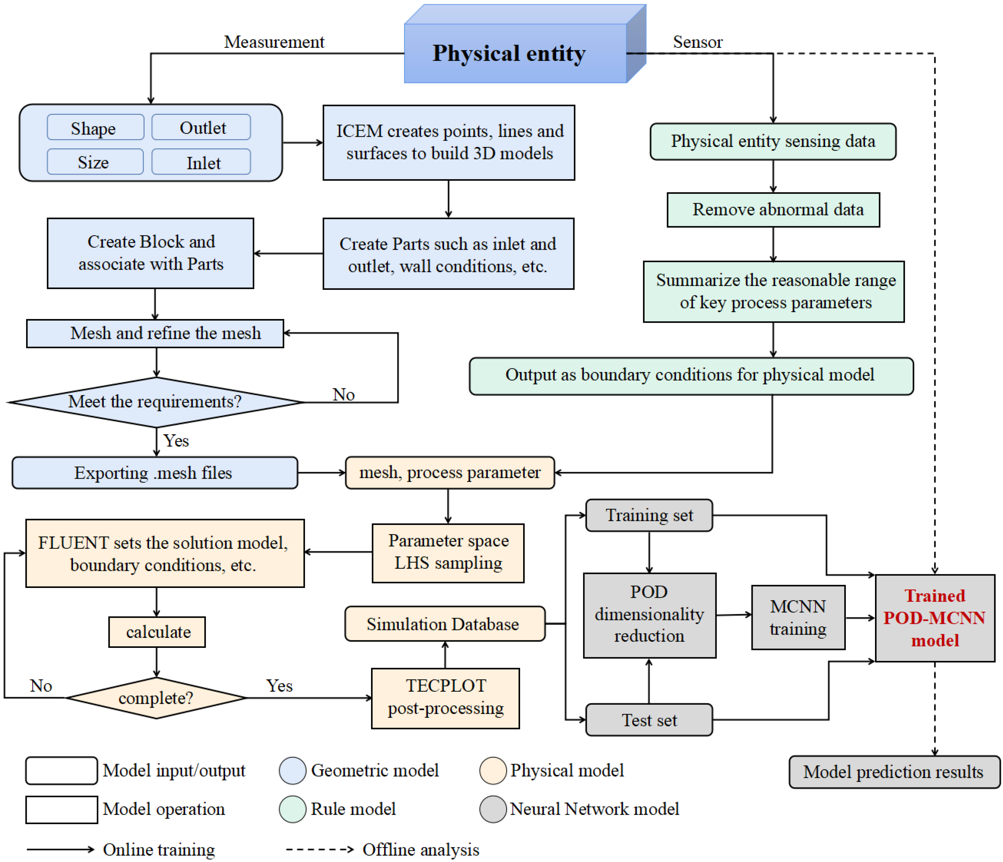
The digital twin model can be divided into two stages: online training and offline analysis. During the online training, through the cooperation of four sub-models, the nonlinear fitting of the neural network is performed on the flow field of the big data. In the offline analysis, it is only necessary to input the condition parameters into the trained model, and the twin model can follow the field data of the physical world for real-time updates to provide real-time monitoring and evaluation of the equipment.

The workflow of the system is shown in Figure 3. The process of creating the CFD digital twin follows the following steps:

• Geometric model

The geometric model of the physical entity is created and meshed using the ANSYS ICEM CFD pre-processing software to restore the physical entity 1:1 ratio and make it reflect its shape, size, boundaries, etc. In the subsequent simulation, the geometric model achieves a complete mirror image of the actual device. The model finally outputs a mesh file.

2.

Rule model

The production operation has a certain process. Based on the historical data from the sensors during the operation of the real physical entity, the process curve for the field operation of the push-plate kiln can be obtained. Then, summarize the normal values of each variable in the production process to determine the variation interval of each parameter.

3.

Physical model

Based on the geometric model and the rule model, use the ANSYS FLUENT solver to simulate the physical process, select an appropriate physical solution model, and set the behavior rules for the parameters, according to the rule model. The behavior rules are reflected in various parameter settings in the software, such as boundary conditions. In this part, the FLUENT automation script is used to generate the flow field data and the TECPLOT is used to post-process the data.

4.

Neural Network Model (POD-MCNN)

The neural network model is the key module to realize CFD offline dynamic analysis. In this part, the flow field big data generated by the physical model are split into training and test sets for the design and training of the neural network model. A well-trained model can respond quickly to the input parameters and output the corresponding CFD results. The detailed process of building the neural network model is described in Section 3.3.

3.3. POD-MCNN Model

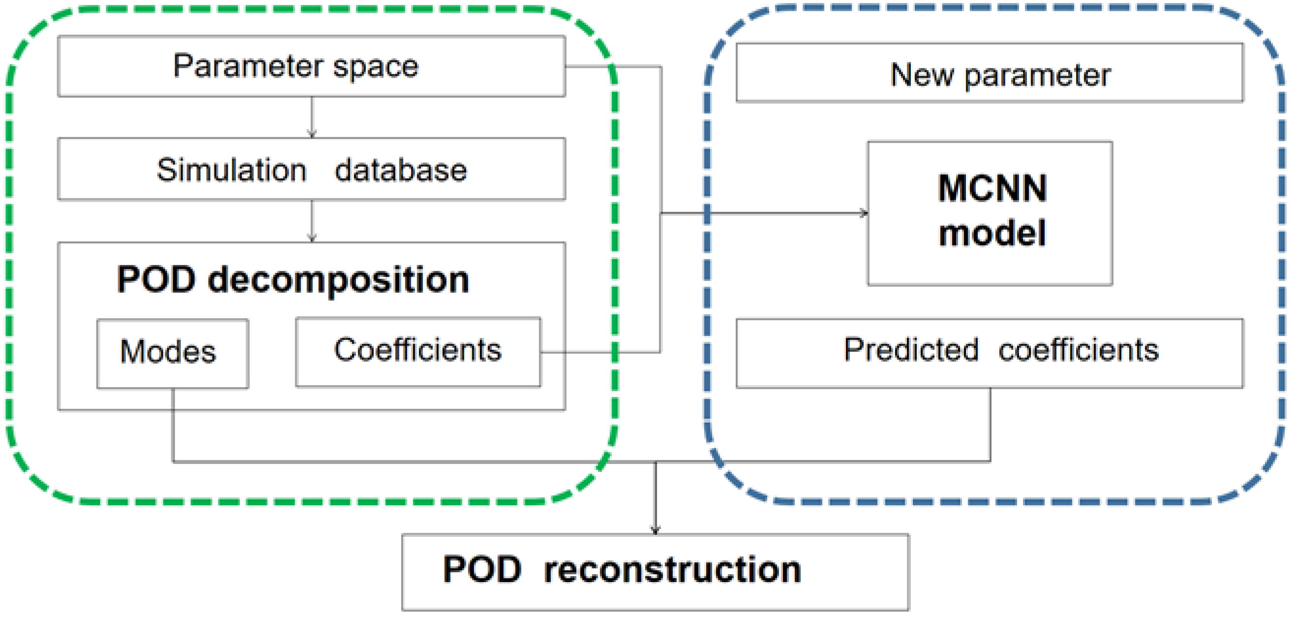
Combining the advantages of POD and CNN, we propose a fast computation method for the flow field, which enables the digital twin to provide a wider range of operating conditions than the simulation and uses it for the real-time monitoring of the temperature and pressure fields of the push-plate kiln. The process is shown in Figure 4. The method can be summarized in three steps: POD dimensionality reduction, MCNN prediction, and POD reconstruction. First, the physical field features of the simulation database are extracted by POD to map the high-dimensional flow field to the low-dimensional space. Then, a surrogate model of input parameters and low-dimensional flow field features is established by a multiscale convolutional neural network to respond to the new input parameters. Finally, data are reconstructed by the basic modes and MCNN prediction data.

3.3.1. POD Extraction of Physical Field Features

The parameter space $C^{\left(i\right)}$ is obtained by the Latin hypercube sampling of each process parameter. The temperature and pressure field data are $X=\left[x_1,x_2,\cdots ,x_r\right]\in {\mathrm{R}}^{\mathrm{n}\times \mathrm{r}}$, where n is the number of nodes in the computational domain and r is the number of samples in the parameter space. The flow field data are high-dimensional, so it is unrealistic to directly map the input parameters $C^{\left(i\right)}$ to the flow field data $X^{\left(i\right)}$ through the neural network. Therefore, it is necessary to use POD to reduce the dimension of the flow field data.

The mean value of the temperature and pressure field is calculated as:

$$\overline{x}=\frac{{{\displaystyle \sum }}_{i=1}^r{X}^{\left(i\right)}}{r}$$

(1)

The standardized sample data are:

$$\overline{X^{\left(i\right)}}=X^{\left(i\right)}-\overline{x}$$

(2)

First, calculate its covariance matrix and n eigenvalues for the standardized sample data, $\overline{X}$, and arrange them from large to small. Then, take the eigenvectors $q^{\left(1\right)},q^{\left(2\right)},\cdots ,q^{\left(m\right)}$ corresponding to the first m eigenvalues to form the mapping matrix U:

$$U={[q^{\left(1\right)},q^{\left(2\right)},\cdots ,q^{\left(m\right)}]}^T$$

(3)

where each eigenvector represents a fundamental mode of the flow field. The reduced order matrix $Y\in R^{m\times r}$ can be obtained with:

$$Y=U\overline{X}$$

(4)

When m is taken to a suitable value, it is guaranteed that:

$$X^{\left(i\right)}\approx U^{\prime }{Y}^{\left(i\right)}+\overline{x}$$

(5)

where $U^{\prime }$ denotes the pseudo-inverse matrix of U. The m-dimensional data $Y^{\left(i\right)}$ can be used to characterize the high-dimensional flow field data $X^{\left(i\right)}$ with a low error rate. By POD modeling, the basic modes and the corresponding coefficient matrix can be obtained, where the basic modes are used for the flow field reconstruction and the coefficient matrix is used for MCNN modeling and flow field prediction, together with the parameter space matrix.

3.3.2. Surrogate Modeling with Multiscale Convolutional Neural Networks

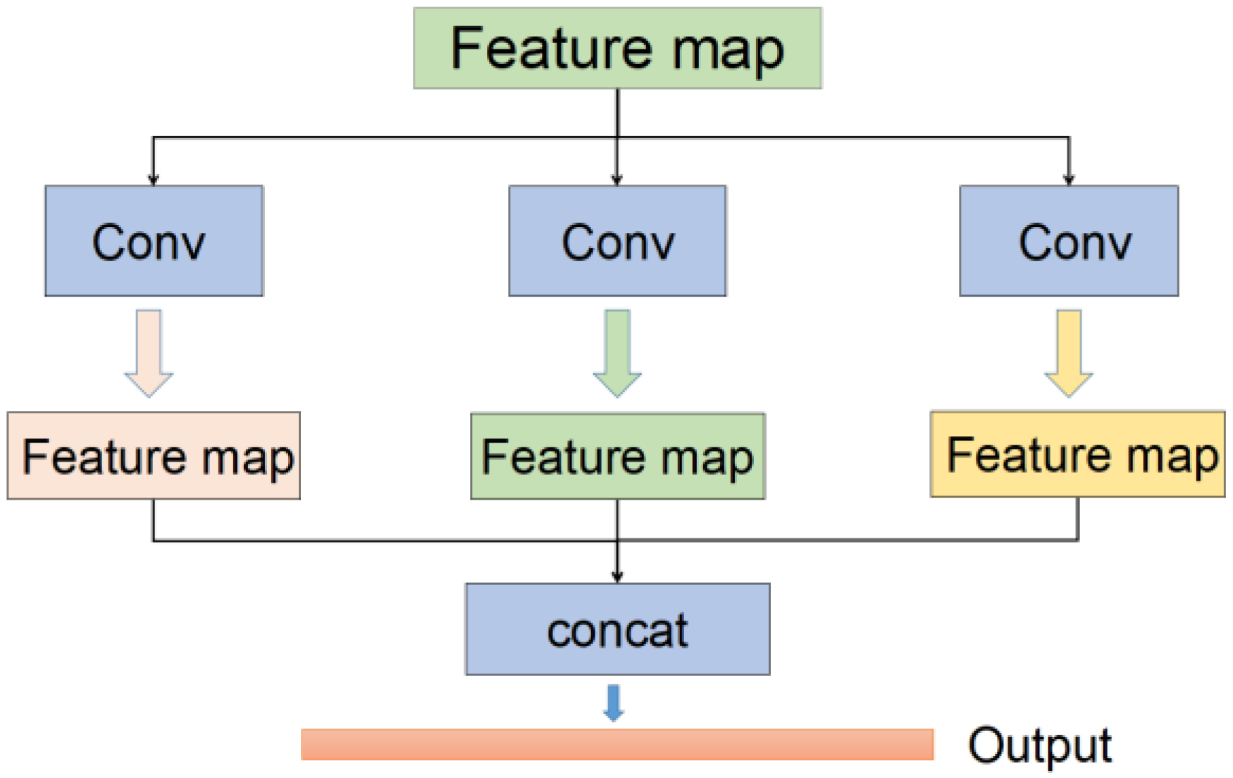
The multiscale convolutional neural network model (MCNN) is designed to accomplish the task of mapping input parameters $C^{\left(i\right)}$ to basic mode coefficient matrices $Y^{\left(i\right)}$. The same feature map will have different expression forms under two different scale spaces. The single-scale convolution process uses the same scale convolution kernel to ex-tract features from the input. It is easy to ignore other precision features, resulting in in-complete feature expression information. In contrast, the multiscale convolutional neural network can use multiple convolution kernels to perform convolution at different scales, with the input to extract features of different scales. Then, these features are fused to achieve the purpose of complementary information. The structure of the network containing three parallel multiscale convolutional layers is shown in Figure 5.

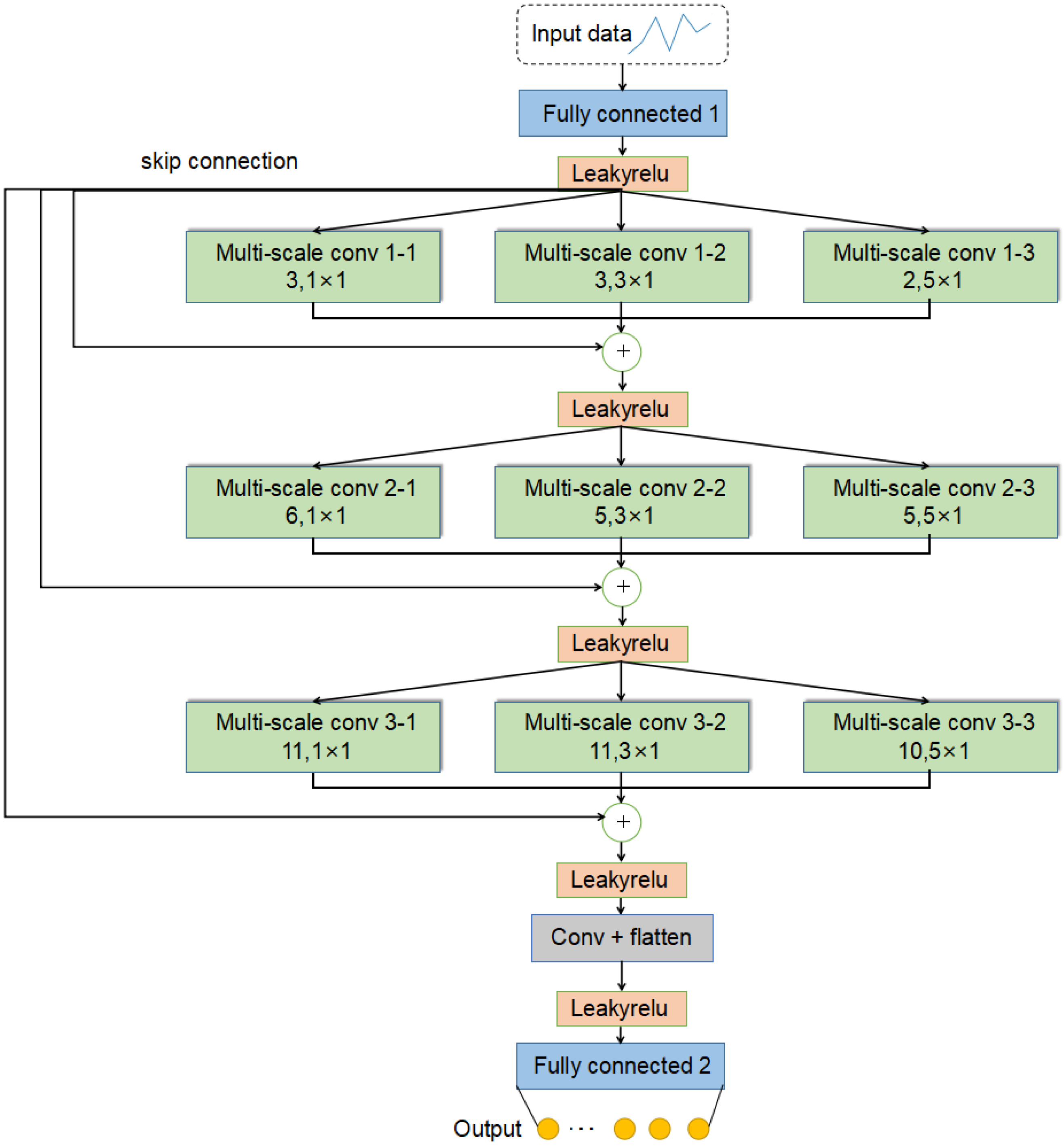
The model input $C=\left(c_1,c_2,\dots ,c_n\right)$ is the parameter obtained from the physical entity sensors through the MQTT protocol. In order to eliminate the influence of the different dimensions between the parameters and speed up the network gradient descent to find the optimal solution, C is standardized. After that, the input parameters are preprocessed through the fully connected neural network $C^{\prime }=f\left(C\right)$, and the low-dimensional input signal is increased in dimension, which is beneficial to extracting the multiscale features of the input signal through the multiscale convolution operation.

The features extracted by convolution kernels at different scales are different. Convolutions with larger kernel sizes have larger receptive fields but are not sensitive to detailed features. Convolutions with smaller kernel sizes can capture detailed features more effectively. Three multiscale convolutional layers are designed in our model, and each layer contains three kernel scales of 1 × 1, 3 × 1, and 5 × 1. These convolutional kernels are used for the multiscale feature extraction of the upper layer output. In addition to the size F of the kernel, the convolutional output is also affected by the kernel step size S, the number of channels n, and the padding size P. The padding operation is to add zeros around the boundaries of the input matrix. The size of the output matrix after the convolution operation can be calculated as:

$$N_{l+1}=\frac{\left(N_l-F+2P\right)}{S}+1$$

(6)

where $N_l$ is the size of the lth layer feature map and $N_{l+1}$ is the size of the l + 1 th layer feature map.

To ensure the high nonlinearity of the proposed model, we use a multi-layer deep structure for our neural network [39]. In addition, the model also fuses the original features with multiscale features through skip connections as the input of the next layer. The features extracted by the multiscale convolutional layer are finally outputted through the fully connected layer. Figure 6 shows the structure of MCNN and

Table 1. Main parameters of multi-scale convolutional neural network.

Layer Name	Output Shape	Kernel Size	Numbers of Kernel	Stride	Padding
Fully connected 1	64	-	-	-	-
Multi-scale conv 1-1	3 × 4	1	3	1	0
Multi-scale conv 1-2	3 × 64	3	3	1	1
Multi-scale conv 1-3	2 × 64	5	2	1	2
Concat	9 × 64	-	-	-	-
Multi-scale conv 2-1	6 × 64	1	6	1	0
Multi-scale conv 2-2	5 × 64	3	5	1	1
Multi-scale conv 2-3	5 × 64	5	5	1	2
Concat	17 × 64	-	-	-	-
Multi-scale conv 3-1	11 × 64	1	11	1	0
Multi-scale conv 3-2	11 × 64	3	11	1	1
Multi-scale conv 3-3	10 × 64	5	10	1	2
Concat	33 × 64	-	-	-	-
Conv + flatten	256	3	2	1	-
Fully connected 2	10	-	-	-	-

lists the main parameters of the network.

The activation function enhances the nonlinear expression ability of the network. LeakyRelu is chosen as the activation function:

$$LeakyRelu\left(x\right)=\{\begin{array}{c}x,x>0\\ ax,x\le 0\end{array}$$

(7)

where $a$ is taken as 0.01. LeakyRelu addresses the possible neuron death problem in Relu. It has a small positive slope in the negative region so that it can perform backpropagation even for negative input values, and solved the problem that the gradient of the Relu activation function disappears.

In general, convolutional neural networks have a pooling layer after convolution. The pooling layer in CNN can reduce the dimensionality of features to some extent, but this is not a necessary operation for CNN [40]. In this experiment, there are not many features after convolution. There is no need to reduce the dimensionality. The pooling process will cause the lack of features extracted by the convolutional layer, which will affect the model’s performance. Therefore, our MCNN structure does not use pooling layers.

3.3.3. Training of Multi-Scale Convolutional Neural Networks

For such a deep model, all operational layers can be considered as the complex function $G$. The network output is:

$$\widehat{Y}=G\left(C,\theta \right)$$

(8)

where $\theta$ are the parameters to be learned in the network. The training of the model is an iterative process driven by model attrition. The parameters of the model are updated by minimizing the difference between the network output and the true value and propagating the error back to each layer of the network. The loss function of our model consists of data loss and a regularizing term. The mean square error is used for the data loss, and the L2-norm is used for the regularizing term. The purpose of including the regularizing term is to prevent the model from overfitting, which leads to the degradation of the generalization performance:

$$L\mathrm{oss}=\frac{1}{N}{\displaystyle \sum }_{n=1}^N{(\widehat{Y}-Y)}^2+\lambda {\displaystyle \sum }_i^M{\theta }_i^2$$

(9)

where $\widehat{Y}$ is the network output; $Y$ is the ground truth; $\lambda$ is the regularization coefficient, which is used to control the strength of regularization; ${\theta }_i\in \theta$ is the parameter to be learned in the network.

During the training process, the purpose of the network is to find a set of optimal parameters $\theta$ to minimize the loss function, denoted as:

$$\theta =\underset{\theta }{argmin}\left(\frac{1}{N}{\displaystyle \sum }_{n=1}^N{(\widehat{Y}-Y)}^2+\lambda {\displaystyle \sum }_i^M{\theta }_i^2\right)$$

(10)

To efficiently train the model, we adopted a mini-batch-based learning strategy, and the batch size was set to 64. The mini-batch training has been shown to effectively improve the generalization performance and significantly reduce the memory cost [41], using the Adam optimization algorithm as the optimization algorithm for the model.

3.3.4. Flow Field Prediction

For a new input parameter, the MCNN model can predict the basic mode coefficients $Y^s$, and then perform POD reconstruction on $Y^s$ to obtain the predicted flow field data.

$$X^s=U^{\prime }{Y}^s+\overline{x}$$

(11)

The results can be directly used as high-precision flow field data to realize the real-time response to the CFD digital twin to the input parameters.

4. Experiments

Section 4.1 presents the structure of the push-plate kiln. Section 4.2 conducts POD flow field decomposition and reconstruction experiments to select an appropriate number of basic modes. Section 4.3 demonstrates the performance of the proposed method on the test data, new data, and failure data. Section 4.4 analyzes the speedup of neural networks compared with CFD simulations. Section 4.5 provides a comparison of different models. The experiments validate the performance of CFD digital twins.

4.1. Push-Plate Kiln

4.1.1. Structure

The push-plate kiln (Figure 7) is heated by electricity. The effective size of the inner space of the furnace body is XYZ = 40,000 mm × 1100 mm × 455 mm. Because the kiln is long, the model is shown properly scaled. Figure 7a shows the geometry of the kiln interior space. According to the temperature, the kiln can be divided into the preheating zone, high temperature zone, and cooling zone. Figure 7b,c show the front and side views of the kiln. The outer wall of the kiln is made of heat-insulating material. There are several electric heating rods above and below the kiln body for heating the push-plate kiln. During the production process, a large amount of nitrogen will be blown into the kiln from the end of the kiln through the pipe, and flow out from the outlet. After an extensive analysis of the historical data of the production line, we found that the temperature values and inlet gas velocity values of the six process critical points have a great impact on the temperature and pressure in the kiln during the production process, so we chose these seven parameters as the variable parameters for generating the simulation dataset.

This paper aims to use CFD digital twins to quickly generate the flow field solution of region 4. In the working process of the push-plate kiln, the heat transfer process in the kiln is a complex heat transfer process, which have the comprehensive functions of heat conduction, convective heat transfer, and radiation heat transfer. To generate the simulation database, we sample the parameter space 1000 times using Latin hypercube sampling (LHS). CFD simulations were performed using Ansys Fluent 19.3 automation scripts, and 1000 CFD flow field solutions were obtained.

4.1.2. CFD Simulation

1.

Mathematical model

CFD is the sub-branch of CAE dealing with fluid flow and thermal processes, wherein the transport of mass, momentum, and energy is modelled via the following equations [19]:

$$\frac{\partial \rho }{\partial t}+\frac{\partial \left(\rho u_j\right)}{\partial x_j}=0$$

(12)

$$\frac{\partial \left(\rho u_i\right)}{\partial t}+\frac{\partial \left(\rho u_i{u}_j\right)}{\partial x_j}=-\frac{\partial p}{\partial x}+\frac{\partial }{\partial x_j}\left(\mu \frac{\partial u_i}{\partial x_j}\right)+S_U$$

(13)

$$\frac{\partial \left(\rho \Phi \right)}{\partial t}+\frac{\partial \left(\rho \Phi u_j\right)}{\partial x_j}=\frac{\partial }{\partial x_j}\left(\mathsf{\Gamma }\frac{\partial \left(\rho \Phi \right)}{\partial x_j}\right)+S_{\Phi }$$

(14)

where $u_i$ and $P$ are the velocity and the pressure, and $\rho$ and $\mu$ are the fluid density and viscosity, respectively. In the scalar equation, $\varphi$ denotes a generic passive scalar (temperature or concentration), and $\mathsf{\Gamma }$ is the diffusivity coefficient. The last terms in Equations (13) and (14) account for sources of momentum and any other quantity, e.g., energy.

2.

Grid generation and solution calculation

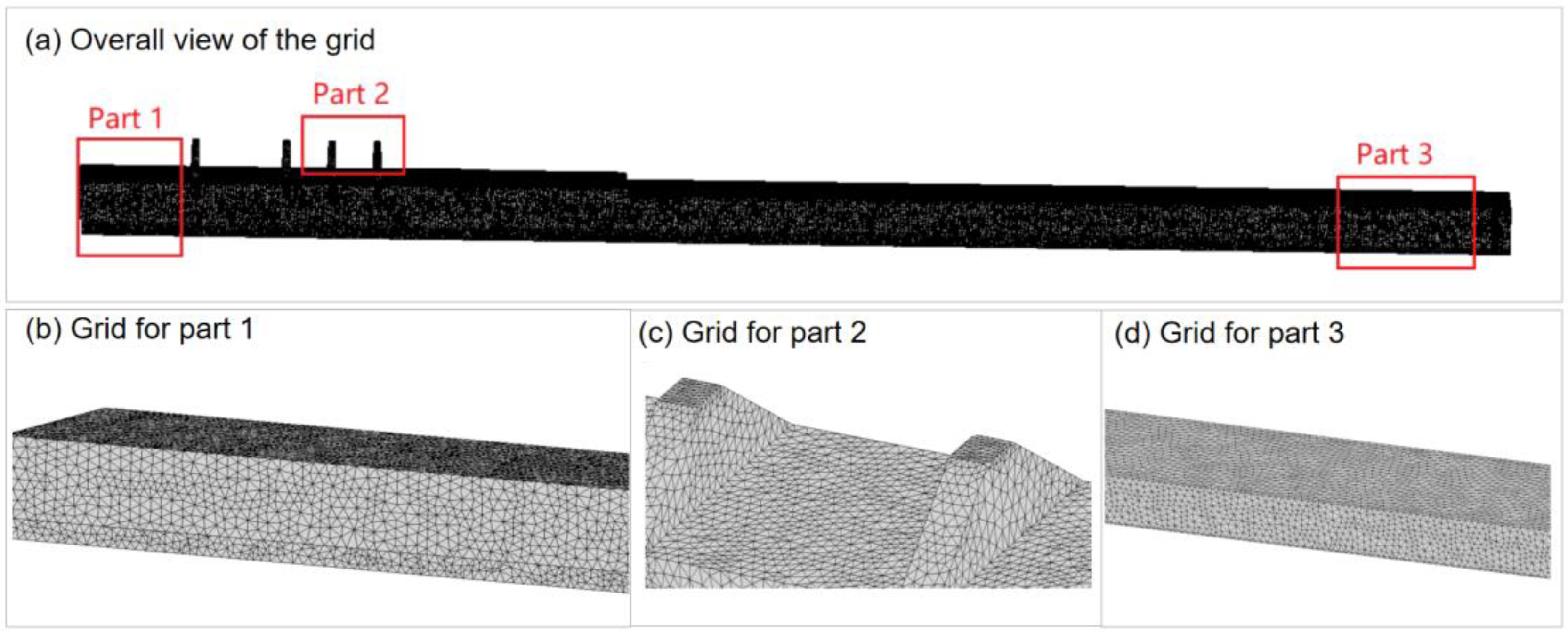
The geometry of the pusher kiln is divided into unstructured meshes. Figure 8a shows the overall view of the mesh, and Figure 8b–d shows the enlarged images of the three parts of the mesh, respectively. The grid consists of approximately 147 k cells.

The airflow adopts the standard k-e model, and the radiation model adopts the discrete coordinate (DO) method.

4.2. POD Flow Field Decomposition and Reconstruction Experiments

The basic modes and corresponding eigenvalues can be obtained by the POD analysis of the simulation data, first arranging the eigenvalues according to the numerical value. The ratio of the sum of eigenvalues corresponding to the q-order fundamental mode to the sum of all eigenvalues is defined as the energy ratio of the q-order fundamental mode. It represents the amount of information contained in the q-order basic mode, which can be used to determine how many modes can contain most of the information in the original flow field. Figure 9 shows the changing trend of the energy contained in the n-order (n < 15) POD basic modes, the abscissa is the order of the basic modes, and the ordinate is the energy ratio.

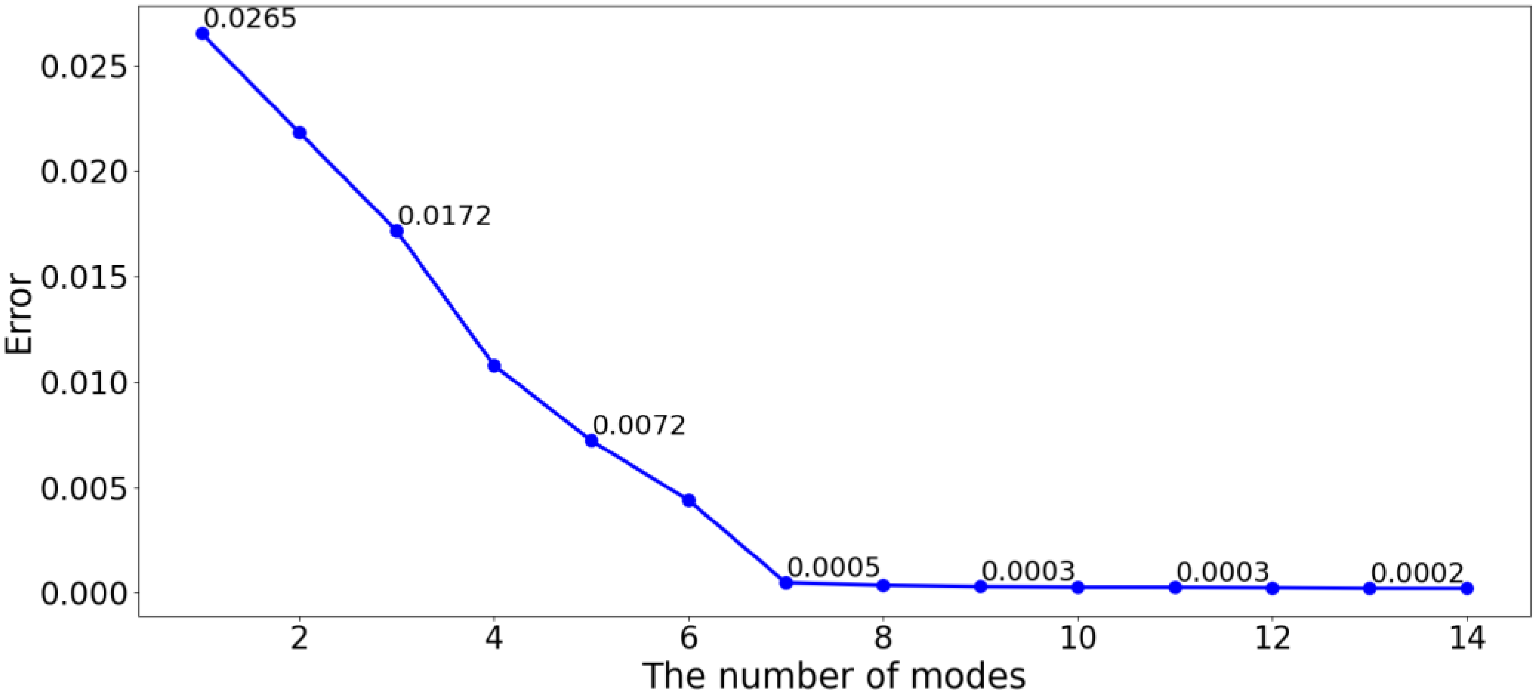
As shown in Figure 9, the energy of the ten basic modes accounts for more than 99.95%, indicating that the flow field characteristics are mainly concentrated in the first ten POD basic modes.

In order to quantitatively analyze the reconstruction effect, 90% of the dataset is used as the training sample for the POD reduction, and the remaining 10% is used as the test sample for POD reconstruction. The reconstruction error of a single test sample is defined as:

$$e=\frac{{{\displaystyle \sum }}_{i=1}^N\left|\frac{\left(a_{pre}^i-a_{real}^i\right)}{a_{real}^i}\right|}{N}$$

(15)

where $a_{pre}^i$ is the predicted data of the ith grid point, $a_{real}^i$ is the real data of the ith grid point calculated by CFD with high accuracy, and $N$ is the number of grid points.

The overall error for all test samples is defined as follows, where T is the number of test samples:

$$E\mathrm{rror}=\frac{{{\displaystyle \sum }}_{k=1}^T{e}^k}{T}$$

(16)

Figure 10 shows the relationship between the number of basic modes and reconstruction error. Obviously, the flow field features are mainly concentrated in the first ten orders. Therefore, after the error analysis of POD reconstruction, the number of basic modes is selected as 10.

4.3. POD-MCNN Model Performance

All experiments were conducted on the same computer equipped with Intel E5 2678V3 processor and NVIDIA RTX 3090 graphics processor. The mean absolute error (MAE) was used to measure the model prediction accuracy, defined as:

$$MAE=\frac{1}{N}{\displaystyle \sum }_{i=1}^N\left(\left|a_{\mathit{pre}}^i-a_{real}^i\right|\right)$$

(17)

4.3.1. Reconstructed Performance on Test Data

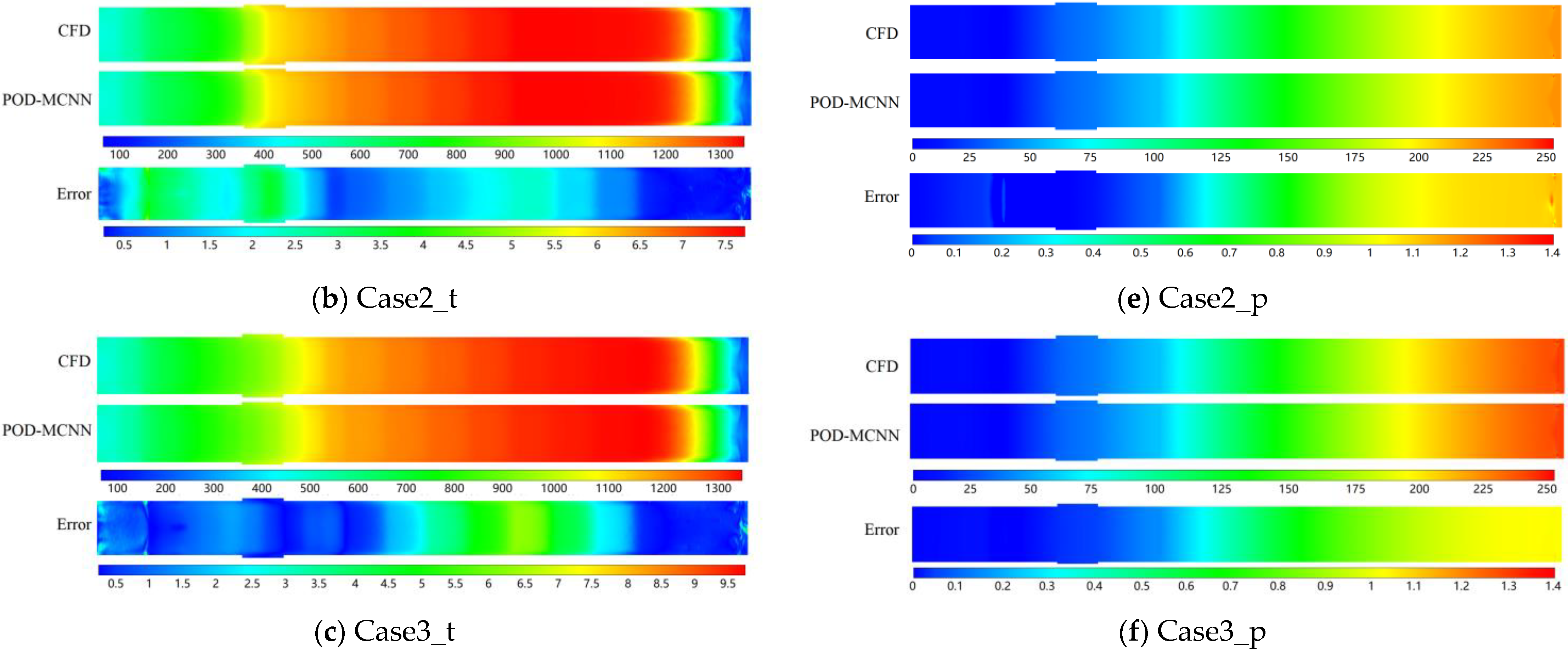
In this section, we evaluate the predictive performance of the network model on the test data. Three cases are selected in the test set to test the model. Figure 11 shows the network model prediction results, numerical simulation results, and absolute error distribution at Z = 350 mm under the three cases. It is obvious that the CFD results and the neural network output look very consistent, so we plot the error. In the error chart, the bluer the color, the smaller the error, and the redder the color, the greater the error.

In addition to this, we calculated the mean absolute error between the predicted results and the CFD calculated results. The results are shown in

Table 2. MAE for three cases on the test data.

Case	MAE t	MAE p
case 1	0.9144	0.4492
case 2	1.5922	0.7042
case 3	1.7068	0.3887

. It can be seen from the data in Table 2 that the average temperature MAE of the three cases is only 1.4045 and the average pressure MAE is only 0.5140, and the error is negligible in engineering applications. The network model performs well on the flow field prediction task on the test data.

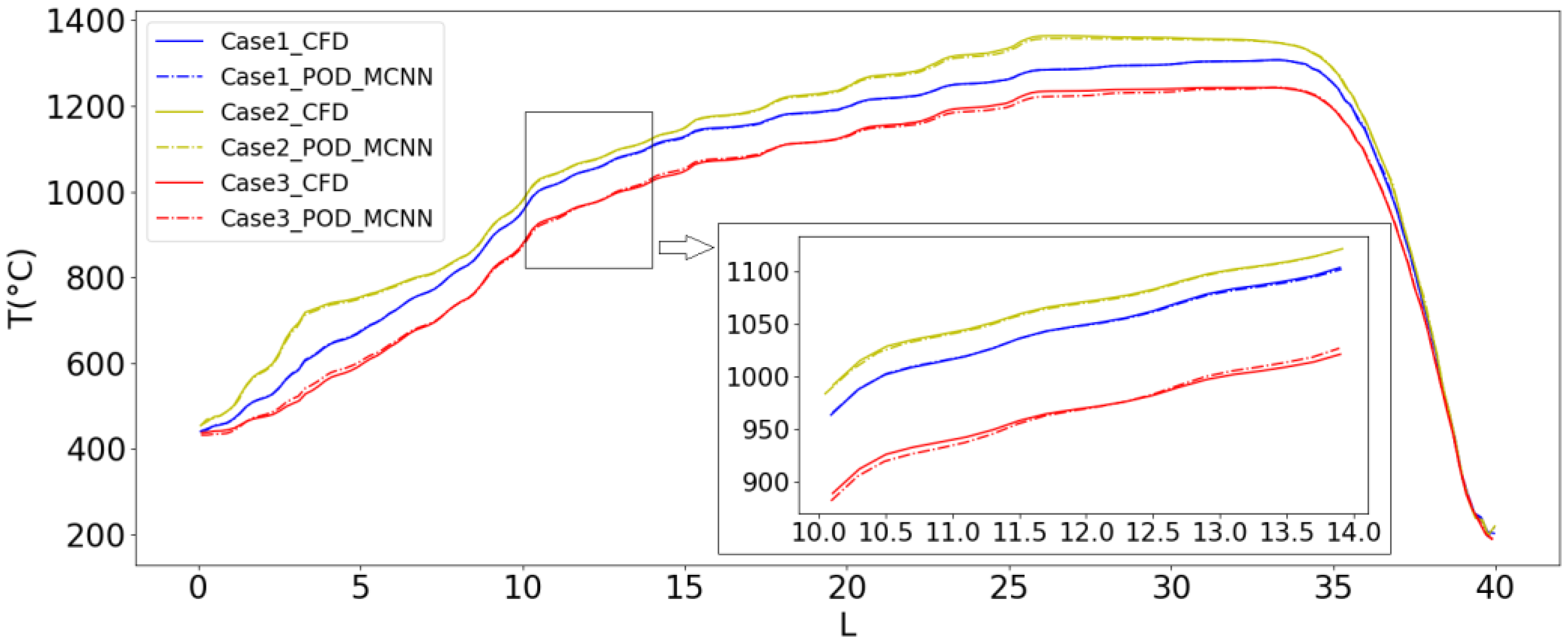
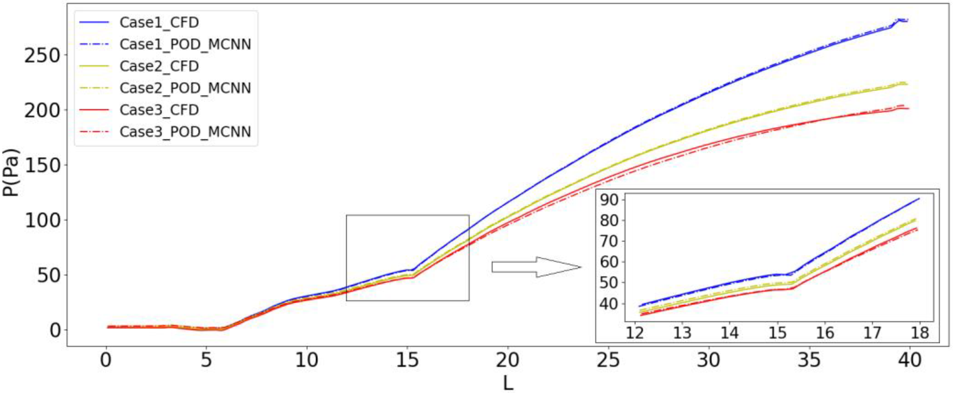
For a working push-plate kiln, the trend of temperature changes is important. Figure 12 and Figure 13 show the comparison between the neural network prediction results and the CFD results of the temperature and pressure trend at Z = 350 mm and Y = 550 mm. It can be seen from the figure that the data trend of the model output is consistent with that of the CFD simulation and almost overlaps.

After training, the model performs well on the temperature and pressure field prediction tasks of the test data, and can predict the flow field data of the test set accurately.

4.3.2. Reconstructed Performance on New Data

To evaluate the interpolation performance of the model, we generated three new cases to test the model. The parameter selection of case1 and case2 is still in the parameter space, but the parameter selection of case3 is not. It can be seen from the data in

Table 3. MAE for three cases on the new data.

Case	MAE t	MAE p
case 1	1.3420	0.4836
case 2	2.5835	0.8289
case 3	3.9226	1.6723

that the MAEs of case1 are 1.3420 and 0.4836. Therefore, the prediction accuracy of the model on new data in the parameter space is not necessarily worse than that of the test set. The MAEs of case3 are 3.9226 and 1.6723, and its error is relatively high because the parameter selection of case3 is not within the parameter range.

Figure 14 and Figure 15 show the comparison between the neural network prediction results and the CFD results of the temperature and pressure trend at Z = 350 mm and Y = 550 mm for three cases on new data. It can be seen from the figure that the data trend of the model output is consistent with that of the CFD simulation.

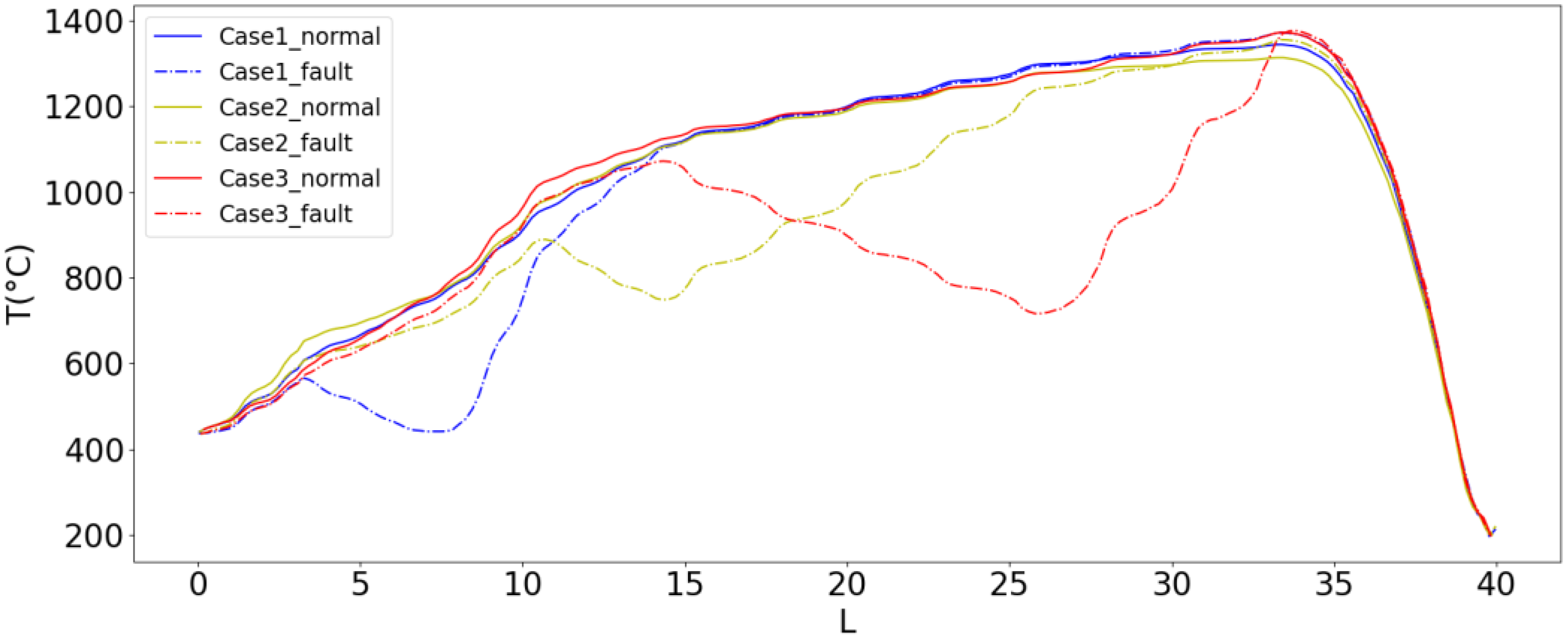
4.3.3. Reconstructed Performance on Fault Data

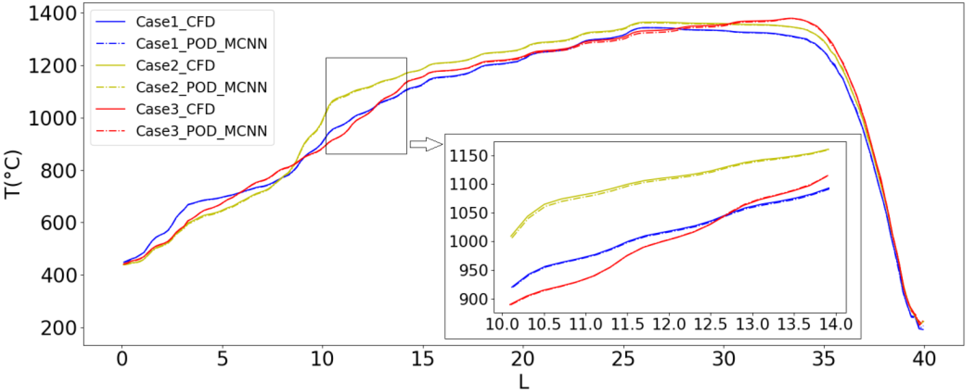
During the use of the push-plate kiln, it does not always work normally, and some-times malfunctions occur. The heating rod has a service life. With the continuous increase in the service time, the heating rod may not be able to provide the set high temperature. When the heating rod is damaged, the temperature will drop sharply, and the data transmitted by MQTT will be significantly less than the normal value of the process. At this time, the heating rod needs to be replaced manually. To evaluate the predictive performance of the model when the failure occurs, we selected three cases (

Table 4. Fault location for three cases.

Case	Fault Location
case 1_fault	preheating zone
case 2_fault	high-temperature zone
case 3_fault	high-temperature zone

) to test the model. The failure of case1 occurs in the preheating zone, and the failures of case2 and case3 occur in the high-temperature zone.

After the model prediction, we extracted temperature trend data (Figure 16). Obviously, when a failure occurs at a critical position in the process, the prediction results of the model will also have a large change. It helps workers in the field detect abnormal conditions and make timely treatment.

4.4. Time Speedup

Table 5. Model time speedup performance.

Method	Time Consumption	Speedup
CFD	1470 s	7350
POD-MCNN	0.2 s

shows the time consumption comparison between CFD numerical calculation and our model. For the prediction of unknown parameters, the trained model takes only 0.2 s to get the result, while CFD simulation takes 1470 s, greatly saving computational cost and time consumption.

4.5. Performance Comparison of Different Models

We compare the MCNN model with other models that demonstrate the importance of various parts of our approach. The three comparison models are the multiscale pooled convolutional neural network (MPCNN), the convolutional neural network with single-scale (CNN), and the fully connected neural network (FNN). The three models can be interpreted as degenerate versions of the MCNN model. MSCNN retains the pooling operation of convolutional neural networks, CNN uses a convolution kernel of one size, and FNN does not use convolution operations.

The training process adopts the same batch size, training times, initial learning rate, and weight decay as the MCNN training. Using the mean squared error on the test set to measure the prediction accuracy of the model:

$$MSE=\frac{1}{N}{\displaystyle \sum }_{n=1}^N{(\widehat{Y}-Y)}^2$$

(18)

where $\widehat{Y}$ is the predicted value of the network output and $Y$ is the true label value. The experimental results are shown in

Table 6. Performance comparison of different models.

Network Model	Number of Parameters	Mean Square Error
FNN	8 k	0.00343
CNN	6 k	0.00264
MPCNN	6 k	0.00306
MCNN	6 k	0.00223

. The proposed model has the smallest mean square error on the test set. Using convolution instead of the full connection greatly reduces the number of parameters of the network. At the same time, the over-fitting phenomenon is improved, and the error is reduced by 35%. Using multi-scale instead of single-scale convolution makes the features extracted by the convolution more abundant, and the error is reduced by 15.5%. Discarding the pooling operation keeps all the features extracted by multi-scale convolution, and the error is reduced by 27.2%.

In conclusion, we use a multiscale convolutional neural network for surrogate modeling. Using multi-scale convolution kernels can extract features of different finesse and improve the feature learning ability of the model. No pooling operation is required in the model, which allows the data features extracted by the convolutional layers to be pre-served, giving the network higher accuracy. Based on high-fidelity simulation and artificial intelligence technology, DT can follow the data of the physical world for real-time updates, providing a data basis for the monitoring, evaluation, optimization, and maintenance of field equipment.

5. Conclusions

In this article, we proposed a CFD digital twin framework. This framework is based on the IoT, CFD simulation, and artificial intelligence technology. It builds the twinned object of the physical entity through the integration of geometric models, rules models, physical models, and neural network models. Digital twins are designed to receive the operating data of physical entities and predict the CFD flow field in real-time to monitor the production status. It allows onsite staff to quickly obtain the CFD simulation results without CFD professional knowledge.

Combined with the characteristics of POD and CNN, we proposed the POD-MCNN model. It performs well for testing data, new data, and fault data. When the key process parameters are abnormal, the model output is also obviously abnormal. It enables on-site workers to adjust the abnormal temperature in time. The model response only requires 0.2 s, which can provide a rapid response at the production site. The speed is greatly accelerated, saving CFD computing costs significantly. Compared with other models, this model has the highest accuracy in predicting the flow field of the push-plate kiln. Through the standardized interface, the data generated by the simulation digital twin can be embedded into the visualization software such as unity to provide the real-time monitoring and evaluation of equipment.

In summary, the simulation digital twin development method proposed in this paper has good accuracy and generalization. Note that the twins in this paper are only used for 3D visual monitoring. The work that can be further explored includes combining the knowledge of production experts and guiding the parameters of the production process through the digital twin.