Reinforcement Learning vs. Computational Intelligence: Comparing Service Management Approaches for the Cloud Continuum

Abstract

Modern computing environments, thanks to the advent of enabling technologies such as Multi-access Edge Computing (MEC), effectively represent a Cloud Continuum, a capillary network of computing resources that extend from the Edge of the network to the Cloud, which enables a dynamic and adaptive service fabric. Efficiently coordinating resource allocation, exploitation, and management in the Cloud Continuum represents quite a challenge, which has stimulated researchers to investigate innovative solutions based on smart techniques such as Reinforcement Learning and Computational Intelligence. In this paper, we make a comparison of different optimization algorithms and a first investigation of how they can perform in this kind of scenario. Specifically, this comparison included the Deep Q-Network, Proximal Policy Optimization, Genetic Algorithms, Particle Swarm Optimization, Quantum-inspired Particle Swarm Optimization, Multi-Swarm Particle Optimization, and the Grey-Wolf Optimizer. We demonstrate how all approaches can solve the service management problem with similar performance—with a different sample efficiency—if a high number of samples can be evaluated for training and optimization. Finally, we show that, if the scenario conditions change, Deep-Reinforcement-Learning-based approaches can exploit the experience built during training to adapt service allocation according to the modified conditions.

1. Introduction

In the last few years, the research community has observed a reshaping of network infrastructures, with a growing interest and adoption of the Cloud Continuum (CC) paradigm. The CC brings together an assortment of computational and storage resources, spreading them across different layers, resulting in the establishment of a unified ecosystem [1]. In this way, users would rely not only on the resources available at the Edge, but could also exploit computing resources provided by Fog or Cloud providers. Consequentially, the CC opens new possibilities for distributing the load of computationally intensive services such as Machine Learning applications, online gaming, Big Data management, and so on [2,3]. It is important to note that all these new innovative options and the inclusion of a plethora of new devices in the ecosystem create a large number of potential threads, which require the adoption of new effective strategies and countermeasures [4]. In such a distributed and heterogeneous environment like the one that the CC brings to the table, effective service management becomes crucial to ensure seamless service delivery and resource optimization.

However, efficiently coordinating resource allocation, exploitation, and management in the CC represents quite a challenge [5]. There is a need for service fabric management solutions capable of efficiently allocating multiple service components using a limited pool of devices distributed throughout the CC, also considering the peculiar characteristics of the resources available at each layer. In addition, the significant dynamicity of the CC scenario calls for adaptive/intelligent orchestrators that can autonomously learn the best allocation for services.

The increasing use of Artificial Intelligence (AI) techniques has led to different and potentially very promising approaches [6], including self-learning ones. Among those, Reinforcement Learning (RL) is the one that for sure has accumulated most of the attention in the research community [7]. RL is a promising Machine Learning area that has gained popularity in a wide range of research fields such as Network Slicing [8], Network Function Virtualization [9], and resource allocation [10]. More specifically, Deep Reinforcement Learning (DRL) has recently emerged as a compelling technique increasingly proposed in service management research [11]. DRL approaches aim to extensively train an intelligent orchestrator to make it capable of effective service management decision-making in various conditions.

Computational Intelligence (CI) solutions represent another promising approach, leveraging smart and gradient-free optimization techniques that can explore a relatively large solution space efficiently [12]. Leveraging CI, it is possible to realize orchestrators that can explore relatively quickly even large solution spaces, thus being able to effectively operate in dynamic conditions with a reactive posture with a minimal re-evaluation lag. Advanced Computational Intelligence solutions seem to be well suited for expensive [13] and dynamic optimization problems [14,15].

Although some metaheuristic performance analyses in Fog environments have been conducted in recent times [16], establishing which of these solutions represents the most-suitable one for service management in the Cloud Continuum is still an open research question. In this paper, we aimed to investigate that question and, towards that goal, compared two DRL techniques, namely the Deep Q-Network (DQN) and Proximal Policy Optimization (PPO), with five Computational Intelligence techniques, namely Genetic Algorithms (GAs), Particle Swarm Optimization (PSO), Quantum-inspired Particle Swarm Optimization (QPSO), Multi-Swarm PSO (MPSO), and the Grey-Wolf Optimizer (GWO), to evaluate their performance for service management purposes.

First, we conducted simulations to train and test these techniques in a realistic Cloud Continuum scenario characterized by limited computing resources at the Edge and Fog layers and unlimited resources at the Cloud. Then, we evaluated the same techniques with a what-if scenario analysis that simulated the outage of Cloud resources. To find a new service allocation, we exploited the experience of the DRL agents without retraining, while for the CI approaches, we performed another optimization run. The results highlighted that PPO was capable of dealing with the modified scenario by distributing the service instances to the Edge and the Fog layer, without retraining the agent, while the DQN was not capable of achieving comparable results. On the other hand, CI algorithms require a cold restart to find an optimal relocation for service component instances.

The remainder of the paper is structured as follows. Section 2 lays out relevant efforts. Section 3 discusses service management in the Cloud Continuum. Then, in Section 4, we present the CI and DRL algorithms that we selected for the comparison outlined in this work. Section 5 describes the methodologies used in this manuscript to solve the service management problem. Then, Section 6 presents the experimental evaluation in which we compared the selected CI and DRL algorithms. Finally, Section 7 concludes the manuscript and outlines potential future works.

2. Related Work

Services and resource management in the Cloud Continuum comprise a challenging research topic that calls for innovative solutions capable of managing the multiple layers of computing resources. The work presented in [17] proposes a resource orchestration framework called ROMA to manage micro-service-based applications in a multi-tier computing and network environment that can save network and computing resources when compared to static deployment approaches. In [18], Pereira et al. propose a hierarchical and analytical model to overwhelm the resource availability problem in Cloud Continuum scenarios. They present multiple use cases to demonstrate how their model can improve the availability and scalability in Edge–Cloud environments. Moreover, the authors in [19] describe a model-based approach to automatically assign multiple software deployment plans to hundreds of Edge gateways and connected Internet of Things (IoT) devices in a continuously changing cyber–physical context.

In recent years, the advent of the Cloud Continuum paradigm has called for new resource management proposals and methodologies to evaluate them. Currently, simulation is one of the most-adopted evaluation techniques in the literature for evaluating the performance of different techniques in Edge–Fog–Cloud scenarios. The authors in [20] propose a simulation approach at different scales to evaluate their Quantum-inspired solution to optimize task allocation in an Edge–Fog scenario. Specifically, they use the iFogSim simulation toolbox [21] for their experiments and make a comparison between their concept and state-of-the-art strategies, showing improvement in prediction efficiency and error reduction. In [22] Qafzezi et al. present an integrated system called Integrated Fuzzy-based System for Coordination and Management of Resources (IFS-CMR), evaluating it by simulation. Thanks to its three subsystems, it integrates Cloud–Fog–Edge computing in Software-Defined Vehicular Ad hoc Networks with flexible and efficient management of the abundance of resources available. The authors in [23] suggest STEP-ONE, a set of simulation tools to manage IoT systems. Specifically, it relies on the Business Process Model and Notation standards to handle IoT applications, defined as a plethora of processes executed between different resources. After an in-depth analysis of the most-relevant simulators in the Edge–Fog scenario and an accurate description of each component of STEP-ONE, they define a hypothetical smart city scenario to evaluate its capabilities at choosing the right process placement strategy. In [24], Tran-Dang et al. present Fog-Resource-aware Adaptive Task Offloading (FRATO), a framework to select the best offloading policy adaptively and collaboratively based on the system circumstances, represented by the number of resources available. In their experiments, they conduct an expanded simulative analysis adopting FRATO to compare several offloading strategies and determine their performance by measuring the service provisioning delay in different scenarios.

Computational Intelligence and RL approaches have been widely adopted to solve service and network management problems. In [25], the authors propose ETA-GA, a Genetic-Algorithm-based Efficient Task Allocation technique, which aims at efficiently allocating computing tasks—according to their data size—among a pool of virtual machines in accordance with the Cloud environment. Furthermore, in [26], Nguyen et al. present a model of a Fog–Cloud environment and apply different metaheuristics to optimize several constraints, such as power consumption and service latency. Through simulation, they legitimize their modeling and prove that approaches based on GAs and PSO are more effective than the traditional ones in finding the best solution to their constraints. The authors in [27] use PSO to solve a joint resource allocation and a computation offloading decision strategy that minimizes the total computing overhead, completion time, and energy consumption. In [28], Li et al. propose a custom PSO algorithm to decide on a computing offloading strategy that aims at reducing system delay and energy consumption. Lan et al. adopt a GA to solve a task caching optimization problem for Fog computing networks in [29]. The authors in [30] propose DeepCord, a model-free DRL approach to Coordinate network traffic processing. They define their problem as a partially observable Markov decision process to exploit their RL approach and demonstrate that it performs much better than other state-of-the-art heuristics in a testbed created using real-world network topologies and realistic traffic patterns. In [31], Sindhu et al. design an RL approach to overcome the shortcomings of Task-Scheduling Container-Based Algorithms (CBTSAs) applied in the Cloud–Fog paradigm to decide the scheduling workloads. By exploiting the Q-Learning, State–Action–Reward–State–Action (SARSA) [32], and Expected SARSA (E-SARSA) [33] schemes, they show that their enhanced version of the CBTSA with intelligent resource allocation achieves a good balance between cost savings and schedule length than previous ones. In [34], the authors present an RL approach influenced by evolution strategies to optimize real-time task assignment in Fog computing infrastructures. Thanks to its ability to avoid incorrect convergence to local optima and the parallelizable implementation, the algorithm proposed overcomes greedy approaches and other conventional optimization techniques. To better visualize the contributions of related efforts, we report a summary in

Table 1. Summary of related efforts.

Reference	Main Contribution	Evaluation/Results
[17]	Resource orchestration for micro-service-based 5G applications	Savings in network and computing resources
[18]	Hierarchical availability model for Edge–Fog–Cloud continuum	Demonstrated improved availability
[19]	Model-based approach for software deployment in Edge gateways	Support for software assignment and deployment in IoT–Edge–Cloud continuum through a fleet concept
[20]	Quantum computing-inspired solution for task allocation	Improvement in prediction efficiency and error reduction
[22]	IFS-CMR: Integrated Fuzzy logic System for Cloud–Fog-Edge computing	Efficient coordination and management in Software-Defined Vehicular Networks
[23]	STEP-ONE: Simulation tools for IoT systems	Evaluation of a monitoring application in a smart city scenario
[24]	FRATO: Framework for Adaptive Task Offloading	Comparative analysis of offloading strategies
[25]	ETA-GA: Genetic Algorithm approach for Task Allocation	Efficient allocation in a simulated Cloud environment
[26]	Metaheuristics for multi-objective task-scheduling problem	Metaheuristics outperformed more-traditional methods
[27]	PSO for resource allocation and offloading strategy for multi-user multi-MEC servers in heterogeneous networks	Minimized computing overhead
[28]	Custom PSO for computing offloading strategy in MEC scenarios	Reduced delay and efficient load balancing of the MEC server
[29]	GA for task caching optimization and mixed-integer nonlinear programming for the maximization of the total utility of the system in Fog computing	Effectiveness of the proposed scheme
[30]	DeepCord: DRL for service Coordination based on real-world conditions	Superior throughput and network utility on realistic network topologies
[31]	RL for task scheduling in a Cloud–Fog ecosystem	Enhanced CBTSA with intelligent resource allocation
[34]	RL for real-time task assignment in Fog computing	Overcomes greedy and conventional methods

.

Although there are many other different works that analyze several CI and RL approaches in depth, there is still a lack of comparative studies that highlight their main differences, advantages, and disadvantages. This work aimed to address this gap by using a simulation-driven approach that brings together both the CI and RL methodologies to find the best solution of a resource optimization problem in a CC scenario.

3. Cloud Continuum

The Cloud Continuum is a term to indicate a plethora of interconnected computing resources deployed at the Edge, Fog, and Cloud computing layer, such as the one shown in Figure 1. Specifically, at the Edge layer, computing resources are mainly represented by MEC servers at Base Stations (BSs), which are responsible for connecting users to the MEC server and the rest of the core network. MEC servers are the closest resources to users that can reach them in a short communication time, i.e., 1–10 ms, thus making them the most-suitable resources for running latency-sensitive applications. On top, the Fog layer can provide higher computing capabilities at a slightly increased communication latency. Finally, at the top layer of the Cloud Continuum, the Cloud layer provides a possibly unlimited amount of resources to run batch processing or applications that do not mandate strict latency requirements.

Concerning the service management perspective, we assumed that there could be multiple service providers that need to install one or more MEC applications using the resources available in the Cloud Continuum. Service providers would ask an infrastructure provider to deploy and manage their applications. Therefore, the infrastructure provider needs to accommodate all provisioning requests using a pool of computing resources distributed throughout the Cloud Continuum. To do so, the infrastructure provider needs to find a proper allocation that can accommodate as many services as possible considering the current conditions, e.g., the resource availability, and the heterogeneity of the computing resources. In addition, the infrastructure provider should also find an allocation that can maximize the performance of the given services.

This is a challenging problem that requires considering the different characteristics of the computing layers, e.g., latency requirements of mission-critical applications, and the limited resources available at the Edge.

The Computational Intelligence and Reinforcement Learning Approaches to Cloud Continuum Optimization

CI and RL are well-used techniques to solve complex service management problems. CI techniques, such as metaheuristics, represent a common solution to explore the search space of NP-Hard problems. Within the resource-management field, these methods have accomplished remarkable results thanks to their capability of efficiently exploring large and complex spaces [35,36]. In particular, CI can provide feasible and robust solutions that are particularly advantageous compared to more-traditional ones [37], which have been effective in some cases, but often struggled with barriers like scalability.

CI represents gradient-free (or black-box) optimization solutions, which perform on a relatively large number of samples across a wide portion of the search space to identify the global optimum. As a result, they cannot be directly applied to a real system, but instead, require some sort of a system model that can be used for evaluation. This is depicted in Figure 2, which provides a model of how CI solutions could be applied to optimize a Cloud Continuum system. As one can see, the real system is paired with a system model, which plays the role of the objective (or target) function to be provided to the CI method.

Let us note that CI solutions play particularly well with the Digital Twin (In this manuscript, we adopted the definition by Minerva et al. [38], which uses the term Digital Twin to refer to the ensemble of the Physical Object (PO), the logical object(s), and the relationship between them.) concept and its application, which researchers and practitioners are increasingly turning their attention to [39], effectively enabling a variant of the model described above, which we depict in Figure 3 [40]. In these cases, the Digital Twin plays the dual role of providing an accurate virtual representation of a physical system and of automatically reconfiguring the real system to operate in the optimal configuration found by the CI solution.

CI solutions essentially build the knowledge of the target function by collecting the outcomes of their sampling in a memory pool that evolves over time to explore the most-promising parts of the search space, usually through algorithms that leverage metaphors from the evolutionary and biological world. This scheme has proven very effective in the optimization of static systems, but requires some additional attention in systems with strong dynamical components, as is often the case in the Cloud Continuum [36,41]. In fact, applying CI solutions to solve dynamic and expensive optimization problems opens the problem of which parts (if any) of the memory need to be invalidated and discarded. This is an open problem that is receiving major attention in the scientific literature [14,15,42].

RL instead takes a significantly different approach. It implements a trial-and-error training phase in which a software agent learns how to improve its behavior by interacting with an environment through a series of actions and receiving a reward that measures how much the decision made by the agent is beneficial to attaining the final goal. Each environment is described as a set of possible states, which reflect all the observations of the agent.

The purpose of RL is to find the optimal policy to be used by the agent for selecting which action to take in each given state. More specifically, we want to learn the set of parameters $\theta$ for a policy ${\pi }_{\theta }$ that maximizes the expected reward:

$$\underset{\theta }{max}J\left({\pi }_{\theta }\right)={\mathbb{E}}_{\tau \sim {\pi }_{\theta }}\left[R\left(\tau \right)\right]$$

(1)

As a result, the reward model is central to the performance of RL solutions, and its correct definition represents a key challenge. Needless to say, there is an interesting ongoing discussion about how to design effective reward models [7,43].

While it is not an optimization solution per se, RL is a rather flexible framework that can be adapted to several different situations. It was developed by design to consider changing environments and does not present the same memory invalidation issues of CI methods in dynamic scenarios. The premise is that policies produced by robust and well-trained RL solutions are applicable to a wide range of conditions. In case of changes in the behavior of the real system, a simple re-evaluation of the policy in an updated state should identify the actions that can be taken to optimize the system configuration—without the need to invalidate (large portions or the entirety of) the acquired knowledge base, as might be the case with CI solutions. RL also has the desirable property of being applicable to directly interact with—and learn from—a real system, as depicted in Figure 4.

However, RL is notoriously considered to be sample-inefficient. In addition, traditional RL algorithms, such as SARSA and Q-Learning, also present scalability issues. They are particularly difficult to adopt in reasonably complex (and realistic) use cases, because of their tabular representation of the functions that map the effectiveness of each possible action in each possible state—which requires a very large amount of experience to be effectively exploited.

Modern Deep Reinforcement Learning (DRL) solutions were proposed to address the scalability issues of traditional RL. With the introduction of neural networks, DRL is capable of effectively dealing with high-dimensional or dynamic problems that are common in most real-world scenarios. More specifically, neural networks act as approximators of the policy (or, more precisely, of the value function V or of the state value function Q that underlies the definition of an RL policy) and have been demonstrated to be very effective in many approaches introduced in the last few years, such as Deep Q-Networks (DQNs) [44] and Trust Region Policy Optimization (TRPO) [45].

Finally, let us note that the research community is paying ever-increasing attention to offline Reinforcement Learning [46,47]. Offline RL represents a promising approach that aims at increasing the sample efficiency of RL through the adoption of a two-phase learning process. First, the RL solution learns in offline mode either from an existing knowledge base of past experiences (such as a trace log) or from a system model (or a Digital Twin). The offline learning phase generates a reasonably effective policy that represents a good starting point to be later fine-tuned during an online training phase in which the RL solution interacts directly with a real system, as depicted in Figure 5. Offline RL is outside the scope of this paper because it is still maturing and the choice of the knowledge base to adopt for a fair and meaningful evaluation, especially in comparison with CI-based approaches, represents a non-trivial issue per se. Nevertheless, we are seriously considering the evaluation of offline RL solutions in Cloud Continuum contexts for future work.

4. Selection of Computational Intelligence and Reinforcement Learning Solutions

There are many CI- and RL-based solutions in the literature, with different characteristics and suitability to specific applications. In this section, we motivate and discuss the selection of five different methods. More specifically, we will focus our investigation on five CI-based solutions: GA, PSO, QPSO, a variant of PSO, MPSO, and GWO, and two DRL-based approaches: DQN and PPO.

The GA represents a robust and flexible optimization solution that can be applied to a wide range of problems, including service management ones [25,48]. While their relatively slow convergence rate in some cases has made them less popular than other CI solutions in recent years, we chose to consider GAs as they represent an important baseline—a gold standard, so to speak. PSO is a simple CI solution that has proven incredibly effective in a wide range of problems, despite requiring careful attention to the parameter setting to facilitate convergence [49]. QPSO is a heavily revised version of PSO inspired by Quantum mechanics, which in our experience has consistently demonstrated solid performance [36,50]. We decided to include PSO and QPSO as relatively simple, robust, and fast-converging CI solutions.

Also, due to the popularity of these approaches within the related literature, we decided to consider the DQN and PPO as representative algorithms for the off-policy and on-policy approaches of RL, respectively. Considering both approaches allows a comprehensive evaluation of RL and could provide valuable insights with respect to different aspects, such as sample efficiency. In Section 6, we will give further details about the specific implementations of the algorithms that we used.

4.1. Genetic Algorithms

The GA is a metaheuristic inspired by biological evolution. The GA considers a population of individuals, which represent candidate solutions for the optimization problem. Each individual has a genotype, which represents its specific coordinate on the search space, and a phenotype, i.e., the evaluation of the objective function in the corresponding coordinate, which represents a “fitness” value capturing how well the individual adapts to the current environment. By evolving populations through selection and recombination, which generate new individuals with better fitness values, the GA naturally explores the search space in an attempt to discover global optima.

More specifically, as the pseudo-code in Algorithm 1 illustrates, the GA implements several phases, beginning with the initial setup of a population. Then, the population is evolved through a number of generations—each one created through a process that involves the selection of individuals for mating and the recombination and mutation of genetic material.

Algorithm 1 Genetic Algorithm.

1: procedure GA (target_function, conf) 2:     $P\leftarrow initialize\_random\_population\left(conf\right)$ 3:     $generation\leftarrow 1$ 4:     $fittest\leftarrow evaluate\_population(P,target\_function)$ 5:     repeat 6:         $P_{next}\leftarrow \varnothing$ 7:         $parents\leftarrow select\_parents(P,conf)$ 8:         for all $p_1,p_2\in parents$ do 9:            $c_1,c_2\leftarrow crossover(p_1,p_2,conf)$ 10:            $P_{next}\leftarrow mutate(c_1,conf),mutate(c_2,conf)$ 11:         end for 12:         $P\leftarrow P_{next}$ 13:         for all $m\in P$ do 14:            $m.fitness\leftarrow target\_function(m.genotype)$ 15:         end for 16:         $fittest\leftarrow {argmax}_{m\in P}m.fitness$ 17:         $generation\leftarrow generation+1$ 18:     until $generation\ge conf.max\_generations$ 19:     return $fittest.genotype,fittest.fitness$ 20: end procedure

Newer generations have a different genetic material, which has the potential to create fitter individuals. With an exchange or recombination of different genes, the evolutionary processes implemented by the GA promote the generation of improved solutions, and their propagation to future generations, at the same time introducing new genes, maintaining a certain degree of diversity in the population—thus preventing premature convergence. This enables the exploration of the search space in a relatively robust and efficient fashion.

The GA presents many customization and tuning opportunities. In fact, the genotype of individuals can be represented in many different ways, such as bitstrings, integers, and real values, and the choice of chromosome encoding represents a crucial aspect of the search performance and convergence speed of the GA [48]. In addition, the GA can use different selection, recombination, and mutation operators. The binary tournament is the most-used selection scheme due to its easy implementation, minimal computational overhead, and resilience to excessively exploitative behaviors, which other selection operators often exhibit [51]. Popular recombination operators include 1-point, 2-point, and uniform crossover, and a plethora of random mutation operators have been proposed in the literature, ranging from bit flip mutation to geometrically distributed displacements with hypermutation [35].

Choosing the specific operators and parameters that control the selection and mutation processes, it is possible to easily modulate the behavior of GAs, making them more explorative or exploitative. Both choices are dependent also on the problem domain and the representation of the chromosomes. The final goal of the GA is to converge to an optimal population, which means that it is not able to produce new offspring notably different from the previous.

4.2. Particle Swarm Optimization and Quantum-Inspired Particle Swarm Optimization

PSO is another metaheuristic consisting of a particle swarm that moves in the search space of an optimization problem and is attracted by global optima. PSO evaluates the objective function at each particle’s current location in a process known as Swarm Intelligence. Each member of the swarm can be a candidate solution, and the way to aggregate the information between all members is the key to better guiding the search in the subsequent steps [52]. Through the years, PSO has drawn much attention thanks to its ease of implementation and the relatively small number of parameters that have to be tuned to obtain a very good balance between exploration and exploitation. However, finding the proper value for each parameter is not a trivial assignment, and many research efforts have been made to reach the current state-of-the-art [53,54].

More specifically, PSO is a relatively simple algorithm, inspired by the behavior of bird flocks [50], based on the exploration of the search space by a swarm of M interacting particles. At each iteration t, each particle i has:

• A current position vector $X_i\left(t\right)=(X_{i,1}\left(t\right),\dots ,X_{i,N}\left(t\right))$, whose components represent the decision variables of the problem;
• A velocity vector $V_i\left(t\right)=(V_{i,1}\left(t\right),\dots ,V_{i,N}\left(t\right))$, which captures the movement of the particles;
• A particle attractor $P_i\left(t\right)=(P_{i,1}\left(t\right),\dots ,P_{i,N}\left(t\right))$, representing the “highest” (best) position that the particle has encountered so far.

The particle movement is, therefore, governed by the following equations:

$$\begin{array}{cc}\hfill V_{i,j}(t+1)=& V_{i,j}\left(t\right)+\hfill \\ \hfill & C_1\ast r_{i,j}\left(t\right)\ast (P_{i,j}\left(t\right)-X_{i,j}\left(t\right))+\hfill \\ \hfill & C_2\ast R_{i,j}\left(t\right)\ast (G_j\left(t\right)-X_{i,j}\left(t\right))\hfill \\ \hfill X_{i,j}(t+1)=& X_{i,j}\left(t\right)+V_{i,j}(t+1)\hfill \end{array}$$

(2)

in which $G\left(t\right)$ is the swarm attractor, representing the “highest” (best) position that the entire swarm has encountered so far, $r_{i,j}\left(t\right)$ and $R_{i,j}\left(t\right)$ are random sequences uniformly sampled in $(0,1)$, and $C_1$ and $C_2$ are constants.

A well-known evolution of PSO is represented by QPSO. In QPSO, all particles have a quantum behavior instead of the classical Newtonian random walks considered by classical PSO. QPSO significantly simplifies the configuration process of PSO, reducing the number of configuration parameters required to only one, i.e., the $\alpha$ contraction–expansion parameter [55], which represents a single “knob” that enables adjusting the balance between the local and global search of the algorithm. Furthermore, QPSO has been demonstrated to overcome the weaknesses of PSO in the resolution of several benchmarks [56], which instead tends to be stuck in local minima. The steps required to implement QPSO are illustrated in Algorithm 2.

Algorithm 2 Quantum-inspired Particle Swarm Optimization.

1: procedure QPSO (target_function, conf) 2:     $particles\leftarrow initialize\_random\_swarm\left(conf\right)$ 3:     $iteration\leftarrow 1$ 4:     $best\leftarrow null$ 5:     repeat 6:         for all p in $particles$ do 7:            $p.val\leftarrow target\_function(p.pos)$ 8:            if $p.val>p.bestval$ then 9:                $p.bestpos\leftarrow p.pos$ 10:                $p.bestval\leftarrow p.val$ 11:            end if 12:            if $p.val>swarm\_bestval$ then 13:                $swarm\_bestpos\leftarrow p.pos$ 14:                $swarm\_bestval\leftarrow p.val$ 15:            end if 16:         end for 17:         $mean\_bestpos\leftarrow \frac{1}{M}{\sum }_{i=1}^{M}particles\left[i\right].bestpos$ 18:         $\overrightarrow{\varphi }\leftarrow rand\left(\right)$ 19:         $\overrightarrow{u}\leftarrow rand\left(\right)$ 20:         $s\leftarrow rand\left(\right)$ 21:         $attr\leftarrow \overrightarrow{\varphi }\ast p.bestpos+(1-\overrightarrow{\varphi })\ast swarm\_bestpos$ 22:         $\delta \leftarrow \alpha \ast |p.pos-mean\_bestpos|\ast ln(1/\overrightarrow{u})$ 23:         $p.pos\leftarrow attr+sign\left(rand\right()-0.5)\ast \delta$ 24:         $iteration\leftarrow iteration+1$ 25:     until $iteration>conf.max\_iterations$ 26:     return $swarm\_bestpos,swarm\_bestval$ 27: end procedure

4.3. Multi-Swarm Particle Optimization

While PSO has been successfully applied in a wide range of applications, it has proven to be less effective in dynamic environments, where it suffers from outdated memory and lack of diversity issues [57]. To address these shortcomings, researchers have started investigating Multi-Swarm PSO (MPSO) constructions [58].

More specifically, MPSO exploits two principle mechanisms for maintaining diversification—and, as a result, avoiding premature convergence and implementing effective exploration throughout the entire search space—in the optimization process: multiple populations and repulsion. Instantiating more than one swarm allows MPSO to simultaneously explore different portions of the search space, thus allowing it to achieve very good performance in the case of multiple optima, i.e., for so-called multi-peak target functions. In addition, MPSO adopts two layers of repulsion: among particles belonging to the same swarm and among all the swarms, to maintain diversity in the exploration process and to avoid premature convergence.

In this context, a particularly successful multi-swarm PSO construction has proven to be the one based on the atom analogy [57]. Taking loose inspiration from the structure of an atom, each swarm is divided into a relatively compact nucleus of neutral (or positively charged) particles and a loose nebula of negatively charged particles that float around the nucleus. This is obtained by moving the neutral portion of the particles according to classical PSO dynamics, i.e., as defined in Equation (2), and the negatively charged rest of the swarm according to quantum-inspired dynamics (Some versions of MPSO use Coulomb-force-inspired repulsion between charged particles, but QPSO dynamics has proven to be computationally simpler and at least just as effective [58]), i.e., as defined in Lines 17–23 of Algorithm 2.

In addition, swarms have and their diversity is preserved by two mechanisms: exclusion and anti-convergence, which lead to a continuous birth-and-death process for swarms. Exclusion implements local diversity, preventing swarms from converging to the same optimum (or peak). If a swarm $S_A$ comes closer than a predefined exclusion radius $r_{excl}$ to another swarm $S_B$, it is killed and a new randomly initialized swarm $S_C$ takes its place. Anti-convergence, instead, implements global diversity, by ensuring that at least one swarm is “free”, i.e., patrolling the search space instead of converging to an optimum. Towards that goal, MPSO monitors the diameter of each swarm, and if all of them fall below a threshold (which is typically dynamically estimated to suit the characteristics of the optimization problem), it kills and replaces one swarm.

Since they have been specifically designed for dynamic optimization problems and are currently considered state-of-the-art solutions in this context [14], MPSO techniques represent a particularly promising candidate for our investigation.

4.4. Grey-Wolf Optimization

GWO is another nature-inspired optimization algorithm based on the leadership hierarchy and hunting mechanism of grey wolves in the wild [59]. The algorithm simulates the social hierarchy and hunting behavior of grey wolves when searching for prey. In GWO, the search agents are grey wolves, which are categorized into four groups: alpha, beta, delta, and omega, which help to guide the pack’s movements.

From a mathematical perspective, the algorithm starts by initializing a population of grey wolves, where each wolf represents a potential solution in the search space. The fitness of each solution is evaluated using a problem-specific objective function. Based on their fitness, the three best solutions are selected as the leading wolves: alpha is the best solution, while beta and delta are the second- and the third-best ones, respectively.

All other candidate solutions are considered as omega, and they will follow the leading wolves in their hunting process. Their position update equations are as follows:

$$\begin{array}{c}{A}^1=2a\times \mathrm{rand}\left(\right)-a\\ C^1=2\times \mathrm{rand}\left(\right)\\ D^{\alpha }=|C^1\times \alpha -X_i|\\ X^1=\alpha -A^1\times D^{\alpha }\end{array}$$

(3)

Similar equations are used to calculate $X^2$ and $X^3$ based on the positions of the beta and delta wolves, respectively. The new position of each wolf is then updated as follows:

$$X_i=(X^1+X^2+X^3)/3$$

(4)

Conceptually, the leading wolves delineate the boundaries of the search space, which typically is defined as a circle. However, the same considerations are still valid if we consider an n-dimensional search space, with a hyper-cube or hyper-sphere instead of a circle. A and C are the components that encourage the wolves to search for fitter prey, helping them avoid becoming stuck in local solutions. Different from A, C does not have any component that decreases linearly, emphasizing ($C>1$) or de-emphasizing ($C<1$) the exploration of each wolf not only during the initial iterations. The algorithm repeats the hunting process for a predefined number of iterations or until convergence is achieved. The alpha wolf represents the optimal solution found by the GWO algorithm. Readers can find a description of the above steps in Algorithm 3.

Similar to PSO, this metaheuristic has no direct relationships between the search agents and the fitness function [59]. This means that penalty mechanisms can be adopted effectively for modeling constraints, thus making GWO particularly suitable for this investigation.

Algorithm 3 Grey-Wolf Optimization (GWO).

1: Initialize the grey wolf population $X_i$ (i = 1, 2, …, n) 2: Initialize a, A, and C, 3: Compute the fitness of each agent 4: $X_{\alpha }$ = best solution found by a wolf 5: $X_{\beta }$ = second-best solution found by a wolf 6: $X_{\delta }$ = third-best solution found by a wolf 7: while t < Max number of iterations do 8:     for each wolf $X_i$ do 9:         Update the position of $X_i$ by Equation (4) 10:     end for 11:     Update a, A, and C 12:     Compute the fitness of each agent 13:     Update $X_{\alpha },X_{\beta },and{X}_{\delta }$ 14:     $t=t+1$ 15: end while 16: Return  $X_{\alpha }$

4.5. Deep Q-Networks

Traditionally, the Q-Learning algorithm builds a memory table, known as the Q-Table, to store Q-Values for all possible state–action pairs. This value represents the return obtained by executing the action $A_t$ at the time step t, which differs from the one indicated by the current policy, and then, following the policy from the next state onward. After each iteration, the algorithm updates the table using the Bellman Equation:

$$Q(S_t,A_t)=(1-\alpha )Q(S_t,A_t)+\alpha \times (R_t+\lambda \times \underset{a}{max}Q(S_{t+1},a))$$

(5)

where S and A are, respectively, the state (or observation) and the action that the agent takes at the time step t, R is the reward received by the agent by taking the action, $\alpha$ is the learning rate, and $\lambda$ is the discount factor, which assigns more value to the immediate rewards, making them more important [60]. Basically, the agent updates the current Q-Value with the best estimated future reward, which expects that the agent takes the best current known action. Although this algorithm is simple and quite powerful to create an RL agent, it struggles in dealing with complex problems composed of thousands of actions and states. A simple Q-Table would not suffice to manage reliably thousands of Q-Values, especially regarding memory requirements.

Deep Q-Learning overcomes the limitations of Q-Learning by approximating the Q-Table with a deep neural network, which optimizes memory usage and gives a solution to the curse-of-dimensionality problem, forming a more-advanced agent called the Deep Q-Network (DQN) [44]. Specifically, the deep neural network receives a representation of the current state as the input, approximates the value of the Q-Value function, and finally, generates the Q-Value for all possible actions as the output. After each iteration, the agent updates the network weights through the Bellman Equation (5). Towards that goal, the DQN first calculates the loss between the optimal and predicted actions:

$$L\left(\theta \right)=L(R_t+\gamma \underset{a}{max}Q(S_t,a),Q(S_t,A_t))$$

where $\gamma$ is the learning rate parameter. The policy parameters are then updated through backpropagation:

$$\theta =\theta -\alpha \nabla L\left(\theta \right).$$

Several types of loss functions have been proposed in the literature, including the mean-squared error and cross-entropy loss.

The trial-and-error mechanism of RL could make off-policy algorithms such as the DQN relatively slow in the training process. To address this problem, the DQN usually relies on experience replay, a replay buffer where it stores experience from the past [61]. This approach collects the most-recent experiences gathered by the agent through its actions in the previous time steps. After each training iteration, the agent randomly samples one or more batches of data from the experience replay buffer, thus making the process more-stable and prone to converge.

Several optimizations have been proposed for the DQN. To stabilize training, DQN solutions often leverage a separate “target” network $Q^{tar}$ to evaluate the best actions to take. $Q^{tar}$ is updated less frequently than the policy network Q, and often through soft (Polyak) updates. Equally often, DQN solutions adopt prioritized experience replay, which assigns higher probabilities to actions that lead to higher rewards when sampling from the experience replay buffer. Finally, different DQN variants have been proposed to mitigate the reward overestimation tendencies of the algorithm [62], such as the Dueling-DQN [63] and Double-DQN [64].

Despite the DQN being one of the first Deep Q-Learning approaches, it is still very widely proposed and highly regarded in the scientific literature, as it has consistently demonstrated a remarkable effectiveness in solving a large number of problems at a reduced implementation complexity.

4.6. Trust Region Policy Optimization and Proximal Policy Optimization

Different from the off-policy nature that characterizes the DQN, Trust Region Policy Optimization (TRPO) is an on-policy RL algorithm that aims to identify the optimal step size in policy gradient descent for convergence speed and robustness purposes [45]. Specifically, TRPO searches for the best way to improve the policy by satisfying a constraint (called the Trust Region), which defines the highest accepted distance between the updated policy and the old one, thus tackling the problems of performance collapse and sample inefficiency typical of policy gradient RL algorithms. To do so, it defines the following surrogate objective:

$$\underset{\theta }{max}{\mathbb{E}}_t\left[{\displaystyle \frac{{\pi }_{\theta }\left(A_t\right|S_t)}{{\pi }_{{\theta }_{old}}\left(A_t\right|A_t)}}{\widehat{A}}^{{\pi }_{{\theta }_{old}}}(S_t,A_t)\right]$$

(6)

where ${\theta }_{old}$ represents the vector of policy parameters before the update and ${\widehat{A}}^{{\pi }_{{\theta }_{old}}}$ is an estimator of the advantage function from the older policy ${\pi }_{{\theta }_{old}}$. It is possible to prove that applying specific constraints to this equation, i.e., bounding the Kullback–Leibler divergence between ${\pi }_{\theta }$ and ${\pi }_{{\theta }_{old}}$, guarantees a monotonic policy improvement and allows the reuse of off-policy data in the training process, making TRPO more-stable and sample-efficient than previous policy-gradient-based RL algorithms [65].

Unfortunately, since TRPO requires a constrained optimization at every update, it could become too complex and computationally expensive (Theoretically, it is possible to transform the constrained optimization step into an unconstrained optimization one through a penalty-based approach. However, in turn, this raises the need to identify a proper penalty coefficient $\beta$ to consider—which is very difficult in practice). These drawbacks call for simpler and more-effective methods for policy gradient descent. Towards that goal, Schulman et al. in [66] introduce the Proximal Policy Optimization (PPO) algorithm. There are two main variants of PPO: PPO-Penalty and PPO-Clip [66,67,68]. PPO-Penalty optimizes a regularized version of Equation (6), introducing an adaptive regularization parameter $\lambda$ that depends on ${\pi }_{\theta }$. On the other hand, PPO-Clip calculates a clipped version of the term:

$${\displaystyle \frac{{\pi }_{\theta }\left(A_t\right|S_t)}{{\pi }_{{\theta }_{old}}\left(A_t\right|S_t)}}$$

and considers as a learning objective the minimum between the clipped and the unclipped versions. This ensures that the update from ${\pi }_{{\theta }_{old}}$ to ${\pi }_{\theta }$ remains controllable, preventing excessively large parameter updates, which could cause massive changes to the current policy, resulting in a performance collapse. More specifically, PPO-Clip leverages a modified version of the surrogate function in Equation (6) as follows:

$$\underset{\theta }{max}{\mathbb{E}}_t[min({\displaystyle \frac{{\pi }_{\theta }\left(A_t\right|S_t)}{{\pi }_{{\theta }_{old}}\left(A_t\right|A_t)}}{\widehat{A}}^{{\pi }_{{\theta }_{old}}}(S_t,A_t),clip({\displaystyle \frac{{\pi }_{\theta }\left(A_t\right|S_t)}{{\pi }_{{\theta }_{old}}\left(A_t\right|A_t)}},1-ϵ,1+ϵ){\widehat{A}}^{{\pi }_{{\theta }_{old}}}(S_t,A_t))]$$

(7)

where function $clip(x,1-ϵ,1+ϵ)$ clips x within the interval $[1-ϵ,1+ϵ]$, with $ϵ$ being a hyperparameter that defines the clipping neighborhood.

Thanks to a more-elegant and -computationally efficient behavior than TRPO, PPO is a particularly interesting solution for deep RL applications. PPO-Clip is arguably the most-interesting variant of PPO: it has proven to be remarkably simple and stable and to work consistently well in a wide range of scenarios, outperforming other algorithms, such as Advantage Actor–Critic [66]. It, thus, represents a very solid candidate to consider in our investigation. For simplicity, in the rest of the manuscript, we use the term PPO to refer to the PPO-Clip algorithm.

5. Service Management in the Cloud Continuum

To address service management in the Cloud Continuum, we describe an optimization problem that aims at finding the proper deployment for a pool of services with different importance. Specifically, we need to activate multiple instances of these services on the resources available throughout the CloudContinuum. Once these instances are activated on a proper device, they will start processing requests. To evaluate the performance of a given deployment configuration, this work adopted the Percentage of Satisfied Requests (PSR), i.e., the ratio between the number of users’ requests that were successfully executed and the total number of requests that were generated in a given time window t.

Specifically, $\mathbb{C}=\{c_1,c_2,\dots ,c_n\}$ is the set of application components that must be allocated by the infrastructure provider on the Cloud Continuum. Each application component has fixed resource requirements $a_{res}$ measured as the number of CPU or GPU cores that should be available for processing on servers. For simplicity, this work assumed that resource requirements for each application $c_i\in C$ are immutable. This assumption is consistent with the related literature [69] and also with modern container-based orchestration techniques, which allow users to specify the number of CPU and GPU cores to assign to each container.

We modeled each application instance as an independent M/M/1 First-Come First-Served (FCFS) queue that processes requests in a sequential fashion. In addition, we considered that queues would have a maximum buffer size, i.e., queues can buffer up to a maximum number of requests. As soon as the buffer is full, the queue will start dropping incoming requests.

We define the computing resources with the set of devices $\mathbb{D}=\{d_1,d_2,\cdots ,d_n\}$, where each $d_i^k\in D$ has an associated type $k\in \{\mathrm{Cloud},\mathrm{Fog},\mathrm{Edge}\}$ to described the server’s characteristics and location. In addition, each device $d_i\in \mathbb{D}$ is assigned with $D_i^{res}$ resources, where $res$ represents the number of computing CPU or GPU cores. Moreover, we assumed that servers at the same computing layer would have an equal computing capacity; thus, servers at the upper computing layers would have higher capacity. At a given time t, the number of resources requested by applications allocated on servers cannot exceed the servers’ capacity $D_i^{res}$.

5.1. Problem Formulation

In this work, we followed the infrastructure provider perspective, which needs to find a deployment for the application components $c\in C$ that maximizes their performance. The infrastructure provider needs to solve the following optimization problem:

$$\begin{array}{cc}\mathrm{arg\; max}& f\left(\mathrm{x}\right)\\ C,D& \end{array}$$

(8)

where C represents the applications that need to be deployed, D is the set of devices where to allocate applications, and x is the service component deployment. Finally, the objective function $f\left(x\right)$ is defined as follows:

$$f\left(x\right)=\sum _{k=1}^n{\Theta }_k\times PSR(c_k,x)$$

(9)

where each ${\Theta }_i$ component is a weight factor that identifies the criticality of a specific application $c_i\in C$ and $PSR(c_i,x)$ is the percentage of satisfied requests for application $c_i$ using configuration x.

It is worth specifying that it is the responsibility of the infrastructure provider to select proper values for the ${\Theta }_i$ components, which represent the utility that an infrastructure provider gains for running a particular application component of type $c_i$. Although it is a relatively simple approach, we believe that it could be reasonably effective to treat several service components with different priorities. Specifically, we envision the ${\Theta }_i$ values to be fixed at a certain time t. To maximize the value of (9), the infrastructure provider needs to improve the current service deployment configuration in a way that the percentage of satisfied requests of the most-important services is prioritized.

To solve the above service management problem, we define a representation that describes how the instances of applications $c_i\in C$ are deployed on device $d\in D$. Therefore, we propose an array-like service configuration with integer values, which extends the one presented in [70] as follows:

$$SC=\left\{X_{c_1,d_1},X_{c_2,d_1},\dots ,X_{c_{k-1},d_{n-1}},\dots ,X_{c_k,d_n}\right\}$$

(10)

where the value of the element $X_{c_i,d_j}$ describes the number of application components of type $c_i$ that are allocated on device $d_j$ for processing requests’ application $c_i$, n is the number of devices, and k the $\left|C\right|$. Finally, to improve the readability of the problem formulation, we show in

Table 2. Summary of notation used for the service management problem.

Symbol	Description
PSR	Percentage of Satisfied Requests
t	Time window in which requests are counted
$\mathbb{C}$	Set of application components
$a_{res}$	Fixed resource requirements of an application component (number of CPU/GPU cores)
$c_i$	An individual application in set $\mathbb{C}$
M/M/1 FCFS queue	Independent queue model for processing requests in First-Come First-Served fashion
$\mathbb{D}$	Set of devices
$d_i^k$	Individual device with type k (Cloud, Fog, Edge)
$D_i^{res}$	Number of computing resources (CPU/GPU cores) for device $d_i$
C	Applications that need to be deployed
D	Set of devices where applications are allocated
x	Service component deployment
$SC$	Array-like service configuration
$X_{c_i,d_j}$	Number of components of type $c_i$ allocated on device $d_j$
n	Number of devices
k	Cardinality of set $\mathbb{C}$

a summary of the notation used.

5.2. Markov Decision Process for Reinforcement Learning Algorithms

Concerning the application of PPO and the DQN to the service management problem, we need to formulate a decision-making problem using the Markov Decision Process (MDP) framework [71]. Specifically, we define two slightly different MDP problems, one specific to the DQN and the other one to PPO. The difference between the two MDPs is related to the definition of possible actions, which can be more elaborated for PPO. Both MDPs define a set of states S, each one defined as the above deployment array (10) to represent the allocation of service components on devices $X_{c_i,d_j}\in C$, and a reward function R, which is the immediate reward $R_a(S,S^{\prime })$ received after performing an action $a\in A$ in a state s.

The main difference between the MDPs is related to how the deployment array in (10) is analyzed and, therefore, the actions that the agent can perform. For the DQN MDP, the agent has to analyze each element of the deployment array sequentially. Specifically, at each timestamp $t_i$, the DQN agent analyzes an element of the deployment array $SC\left[t_i\right]$, starting from the beginning to the end. When analyzing $SC\left[t_i\right]$, the agent performs an action $a\in A$ on the element $SC\left[t_i\right]$ to modify the active instances for application components $c_i$ on $d_j$, the value of $X_{c_i,d_j}\in C$. To do so, the agent can either (i) do nothing, (ii) activate up to two new instances, or (iii) deactivate up to two instances. Let us note that we encoded these actions as integer values in $[0,5]$.

Instead, for PPO, A has the shape of a multi-discrete action space, i.e., a vector that extends the discrete action space over a space of independent discrete actions [72]. Our proposal consists of two vectors of choices: to perform the first choice, the agent picks an element of C, corresponding to the number of active instances for service component $c_i$ on device $d_j$. Then, for the second choice, the agent modifies the number of active instances to improve the current allocation according to the three actions described for the DQN. Therefore, according to this formulation, the PPO agent does not scan the deployment array in a sequential fashion; instead, it can learn a smarter way to improve the overall value of (9).

Concerning the reward definition, we modeled the reward by performing an action a in state S bringing to a new state $S^{\prime }$, i.e., $R_a(S,S^{\prime })$, as the difference in (9) calculated between two consecutive time steps. Specifically, with this reward function, we want to verify if a specific action can improve or not the value of (9).

$$R_a(S,S^{\prime })=R{\ast }_a(S,S^{\prime })-\Phi$$

(11)

Specifically, $R{\ast }_a(S,S^{\prime })$ and $\Phi$ are defined as:

$$R{\ast }_a(S,S^{\prime })=f\left(S^{\prime }\right)-f\left(S\right)$$

(12)

$$\Phi =\#infeasible\ast \gamma$$

(13)

where $f\left(S^{\prime }\right)$ and $f\left(S\right)$ are the objective functions calculated, respectively, in states $S^{\prime }$ and S and $\Phi$ is the penalty quantified in the number of accumulated infeasible allocations during the simulation multiplied by a facto $\gamma$, which we set to $0.1$. If there is an improvement from one time step to the next one ($R{\ast }_a(S,S^{\prime })>0$), the agent receives an additional bonus of $3.0$ as compensation for its profitable move. Otherwise, the action taken is registered as a wrong pass since it is not remunerative in improving the objective function calculated previously. If the agent reaches an amount of 150 wrong passes, the training episode terminates immediately and resets the environment to the initial state.

5.3. Target Function Formulation for Computational Intelligence Algorithms

CI techniques require their adopters to define a “fitness function” or “evaluation function” to drive the optimization process. One of the advantages of these techniques is that is possible to use the objective function directly as the fitness function. However, it is common to add additional components, (e.g., a penalty component) to guide the optimization process to better solutions.

For this work, we adopted two different configurations for the Computational Intelligence techniques. Specifically, we used a baseline configuration, namely “GA”, “PSO”, “QPSO”, “MPSO”, and “GWO”, which uses as the fitness function the objective function $f\left(x\right)$, and another configuration called Enforced ConstrainT (ECT), namely “GA-ECT”, “PSO-ECT”, “QPSO-ECT”, “MPSO-ECT”, and “GWO-ECT”, which instead takes into account the infeasible allocations generated at a given iteration as a penalty in the fitness function $J\left(x\right)$:

$$J\left(x\right)=f\left(x\right)-\Phi$$

(14)

where $f\left(x\right)$ is the target function (i.e., the problem objective) and $\Phi$ is the penalty component visible in Equation (13). Different from the baseline configuration, the ECT configuration would also minimize the number of infeasible allocations while maximizing the PSR. Finally, let us note that the ECT approach reconstructs the operating conditions of the RL algorithms and forces both metaheuristics to respond to the same challenge, thus enabling a fair comparison with the DQN and PPO.

6. Experiments

As part of this section, we want to compare the RL and Computational Intelligence approaches in finding the best resource management solution in our proposed scenario. As mentioned before, we argue that metaheuristic approaches could be very effective tools in exploring the parameters’ search space and providing near-optimal configuration solutions. Furthermore, these approaches are less inclined to suffer from the inefficient sampling curse. RL methodologies instead provide autonomous learning and adaptation at the expense of a superior sample inefficiency. Therefore, they do a better job in scenarios characterized by high dynamicity and sudden variations, which often induce metaheuristics to have poor performances, forcing them to a new training phase.

To compare the CI and RL approaches for service management, we define a use case for a simulator capable of reenacting services running in a Cloud Continuum scenario. We built this simulator by extending the Phileas simulator [73] (https://github.com/DSG-UniFE/phileas (accessed on 21 September 2023)), a discrete event simulator that we designed to reenact Value-of-Information (VoI)-based services in Fog computing environments. However, even if, in this work, we did not consider the VoI-based management of services, the Phileas simulator represented a good commodity to evaluate different optimization approaches for service management in the Cloud Continuum. In fact, Phileas allows us to accurately simulate the processing of service requests on top of a plethora of computing devices with heterogeneous resources and to model the communication latency between the parties involved in the simulation, i.e., from users to computing devices and vice versa.

To make this comparison, we evaluated the quality of the best solutions generated with respect to the objective function (9), but also in terms of sample efficiency, i.e., the number of evaluations of the objective function. Finally, we evaluated whether these approaches can work properly when environmental conditions change, e.g., the sudden disconnection of computing resources.

6.1. Use Case

For this comparison, we present a scenario to be simulated in Phileas that describes a smart city that provides several applications to its citizens. Specifically, the use case contains the description of a total of 13 devices distributed among the Cloud Continuum: 10 Edge devices, 2 Fog devices, and a Cloud device with unlimited resources to simulate unlimited scalability. Along with the devices’ description, the use case defines 6 different smart city applications, namely: healthcare, pollution-monitoring, traffic-monitoring, video-processing, safety, and audio-processing applications, whose importance is described by the $Theta$ parameters shown in

Table 3. Weight parameters used for the objective function.

$\Theta$ Weight	Service Type
1	Healthcare, Video, Safety
0.5	Pollution, Traffic, Audio

.

To simulate a workload for the described applications, we reenacted 10 different groups of users located at the Edge that generate requests according to the configuration values illustrated in

Table 4. Service description: time between request generation and compute latency modeled as exponential random variables with rate parameter $\lambda$ for each service type and resource occupancy.

Service Type	Time Between Req. Gen. ($\mathit{\lambda }$)	Compute Latency ($\mathit{\lambda }$)	Resource Consumption
Healthcare	$1/120$ (ms)	$1/150$ (ms)	$4.5$ (cores)
Pollution	$1/45$ (ms)	$1/250$ (ms)	$3.5$ (cores)
Traffic	$1/40$ (ms)	$1/300$ (ms)	$3.5$ (cores)
Video	$1/100$ (ms)	$1/225$ (ms)	$6.0$ (cores)
Safety	$1/100$ (ms)	$1/150$ (ms)	$4.0$ (cores)
Audio	$1/25$ (ms)	$1/200$ (ms)	$3.0$ (cores)

. It is worth specifying that the request generation is a stochastic process that we modeled using 10 different random variables with an exponential distribution, i.e., one for each user group. Furthermore, Table 4 also reports the computed latency for each service type. As for the time between message generation, we modeled the processing time of a task by sampling from a random variable with an exponential distribution. Let us also note that the “compute latency” value does not include queuing time, i.e., the time that a request spends before being processed. Finally, the resource occupancy indicates the number of cores that each service instance requires to be allocated on a computing device.

We set the simulation to be 10 s long, including 1 s of warmup, to simulate the processing of approximately 133 requests per second. Finally, we report the intra-layer communication model in

Table 5. Communication latency configuration for the Cloud Continuum use case.

Layers	Edge	Fog	Cloud
Edge	$\mu =5.00$ (ms)	$\mu =15.00$ (ms)	$\mu =100$ (ms)
	$\sigma =3.00$ (ms)	$\sigma =5.00$ (ms)	$\sigma =6.00$ (ms)
Fog		$\mu =5.00$(ms)	$\mu =80.00$ (ms)
		$\sigma =3.00$ (ms)	$\sigma =8.00$ (ms)
Cloud			$\mu =17.00$ (ms)
			$\sigma =7.00$ (ms)

, where each element is the configuration for a normal random variable that we used to simulate the transfer time between the different layers of the Cloud Continuum.

Concerning the optimization approaches, we compared the open-source and state-of-the-art DQN and PPO algorithms provided by Stable Baselines3 (https://github.com/DLR-RM/stable-baselines3 (accessed on 21 September 2023)) with the GA, PSO, QPSO, MPSO, and GWO. For the metaheuristics, we used the implementations of a Ruby metaheuristic library called ruby-mhl, which is available on GitHub (https://github.com/mtortonesi/ruby-mhl (accessed on 21 September 2023)).

6.2. Algorithms Configurations

To collect statically significant results from the evaluation of the CI approaches, we decided to collect the log of 30 optimization runs. Each optimization run consisted of 50 iterations of the metaheuristic algorithm. This was to ensure the interpretability of the results and to verify if the use of different seeds can significantly change the outcome of the optimization process. At the end of the 30 optimization runs, we measured the average best value found by each approach to verify which one performed better in terms of the value of the objective function and sample efficiency.

Delving into the configuration details of each metaheuristic, for the GA, we used a population of 128 randomly initialized individuals, an integer genotype space, a mutation operator implemented as an independent perturbation of all the individual’s chromosomes sampled from a geometric distribution random variable with a probability of success of 50%, and an extended intermediate recombination operator controlled by a random variable with a uniform distribution in $[0.5,1.5]$ [74]. Moreover, we set a lower and an upper bound of 0 and 15, respectively. At each iteration, the GA generates the new population using a binary tournament selection mechanism, in which we applied the configured mutation and recombination. For PSO, we set a swarm size of 40 individuals randomly initialized in the float search space $[0,15]$ and the acceleration coefficients C1 and C2 to 2.05. Then, for QPSO, we configured a swarm of 40 individuals randomly initialized in $[0,15]$ and a contraction–expansion coefficient $\alpha$ of 0.75. These particular parameter configurations have shown very promising results in different analyses made in the past [36,75], so we decided to keep them also for this one.

For GWO, we set the population size to 30 individuals and the same lower and upper bounds of 0 and 15. Then, a different configuration was used for MPSO, where we set the initial number of swarms to 4, each one with 50 individuals, and the maximum number of non-converging swarms to 3. Readers can find a summary table containing the configuration for each CI algorithm provided in

Table 6. CI algorithms configuration for the experiments.

Parameter/Setting	Description
General
Optimization runs	30 runs
Iterations per run	50 iterations
Objective	Average best value and sample efficiency
Bounds	[0, 15]
GA
Population size	128 individuals
Genotype	Integer
Mutation operator	Random perturbation
Mutation probability	Geometric random variable with a probability of success of 50%
Recombination operator	Extended intermediate recombination
Recombination probability	Uniform random variable in $[0.5,1.5]$
Recombination threshold	40%
Selection mechanism	Binary tournament
PSO
Swarm size	40 individuals
Search space	Float
Acceleration coefficients C1 and C2	2.05
QPSO
Swarm size	40 individuals
Contraction–expansion coefficient ($\alpha$)	0.75
GWO
Population size	30 individuals
Bounds	[0, 15]
MPSO
Initial swarms	4 swarms
Individuals per swarm	50 individuals
Maximum non-converging swarms	3

.

Regarding the DRL algorithms, we implemented two different environments to address the different MDP formulations described above. Specifically, the DQN scans the entire allocation array sequentially twice for 156 time steps, while PPO uses a maximum of 200 time steps, which correspond to their respective episode length. Since the DQN implementation of Stable Baselines3 does not support the multi-discrete action space as PPO does, we chose this training model to ensure the training conditions were as similar as possible for both algorithms. As previously mentioned, during a training episode, the agent modifies how service instances are allocated on top of the Cloud Continuum resources. Concerning the DRL configurations, we followed the guidelines of Stable Baseline3 for one-dimensional observation spaces to define a neural network architecture with 2 fully connected layers with 64 units each and a Rectified Linear Unit (ReLU) activation function for the DQN and PPO. Furthermore, we set for both the DQN and PPO a training period of 100,000 time steps long. Then, to collect statistically significant results comparable to the ones of the CI algorithms, we tested the trained models 30 times.

6.3. Results

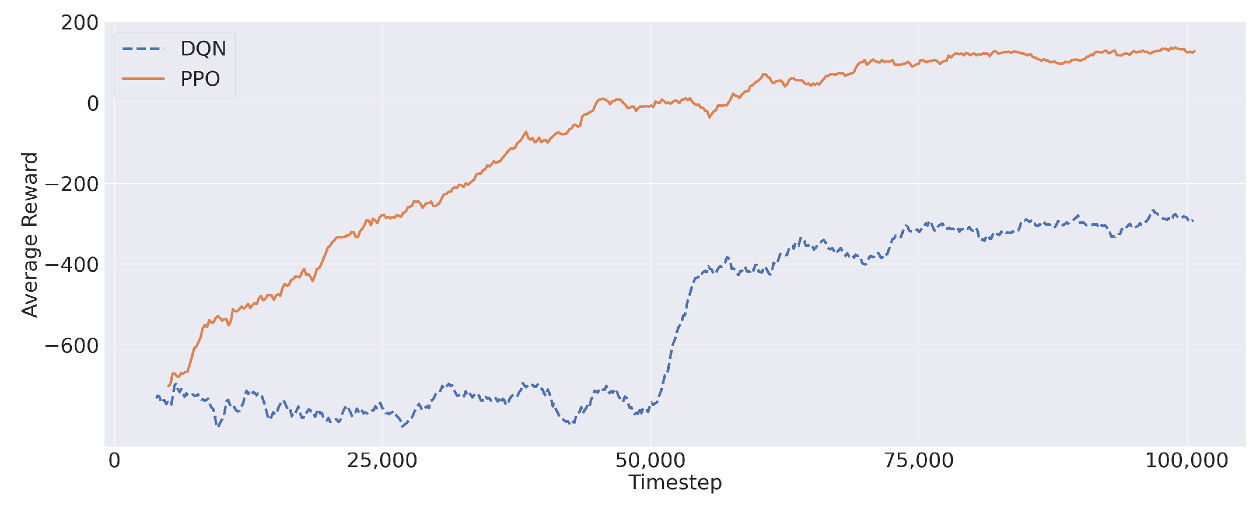
For each optimization algorithm, we took note of the solution that maximized the value of (9), also paying particular attention to the percentage of satisfied requests and service latency. Firstly, let us report the average reward during the training process obtained by PPO and the DQN in Figure 6. Both algorithms showed a progression, in terms of average reward, during the training process. Furthermore, Figure 6 shows that the average reward converged to a stable value before the end of the training process, thus confirming the validity of the reward structure presented in Section 3. In this regard, PPO showed a better reward improvement, reaching a maximum near 200. Differently, the DQN remained stuck in negative values despite a rapid reward increase (around Iteration 50,000) during the training session.

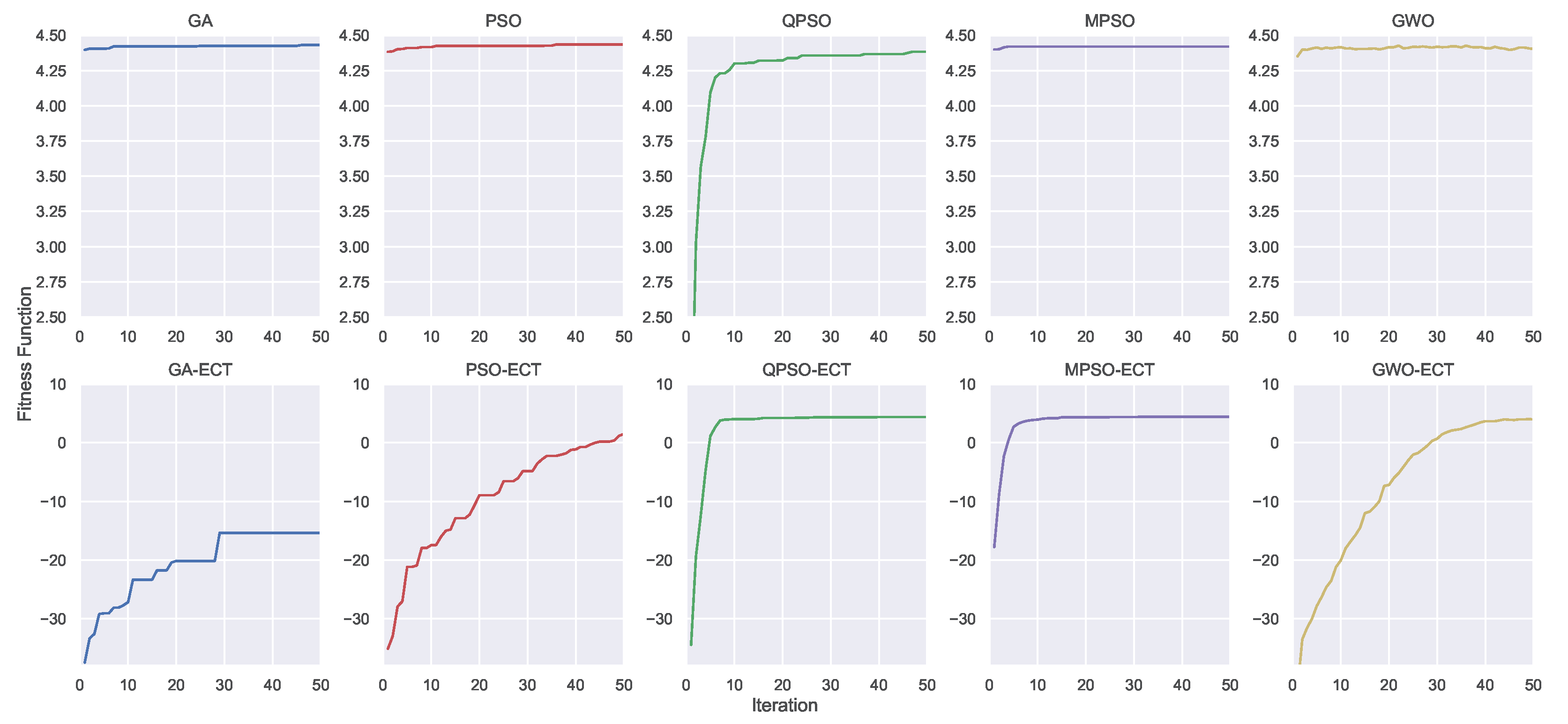
Aside from the DRL training, let us show the convergence process of the CI algorithms in Figure 7, which is an illustrative snapshot of the progress of the optimization process. Specifically, Figure 7 shows the convergence process of one of the 30 optimization runs and visualizes on the top the GA, PSO, QPSO, MPSO, and GWO, while on the bottom their constrained versions the GA-ECT, PSO-ECT, QPSO-ECT, MPSO-ECT, and GWO-ECT. For all metaheuristics displayed in the top row, it is easy to note how they can converge very quickly except for QPSO, which showed an increasing trend throughout all 50 iterations. Instead, considering their ECT variants, the GA, PSO, and GWO struggled a bit in dealing with their imposed constraints. In contrast, QPSO-ECT and MPSO-ECT demonstrated very similar performance compared to the previous case. Notably, these two algorithms did not appear to be negatively affected by the introduction of the penalty factor, and they were still able to find the best solution overall without significant difficulty. In this regard, it is worth noting that MPSO makes use of four large swarms of 50 particles, i.e., at each iteration, the number of evaluations of the objective function was even larger than the GA, which was configured with 128 individuals.

To give a complete summary of the performance of the adopted methodologies (CI and DRL), we report in

Table 7. Comparison of the average best solutions and the sample efficiency for the chosen algorithms.

Algorithm	Objective Function		Generation		Sample Efficiency	Infeasible Allocation
	Avg	Std	Avg	Std		Avg	Std
PPO	4.1004	0.1567	_	_	21.43 (18)	18.83	6.39
DQN	3.7895	0.51762	_	_	24.17 (40.95)	448.43	83.27
GA	4.4288	0.0027	28.07	14.9088	3593	476.27	34.20
PSO	4.3221	0.0051	34.73	10.4977	1389	425.67	38.67
QPSO	4.4255	0.0074	30.9	14.1941	1236	482.53	204.10
MPSO	4.4313	0.0060	32.3667	12.7617	6473	406.07	209.89
GWO	4.4279	0.00600	31.17	14.1326	935	287.03	32.66
GA-ECT	4.1467	0.2829	39.7	8.0049	5082	204.40	11.83
PSO-ECT	4.3325	0.1014	49.57	0.6789	1983	31.97	8.28
QPSO-ECT	4.3589	0.0560	44.63	6.4513	1785	0.0	0.0
MPSO-ECT	4.3981	0.0254	41.9	7.8052	8380	0.0	0.0
GWO-ECT	4.3856	0.0324	46.9	2.3540	1407	0.0	0.0

the average and the standard deviation we collected along the 30 optimization runs. More specifically, Table 7 reports the results for the objective function, the number of generations needed to find the best objective function, and the average number of infeasible allocations associated with the best solutions found. Let us specify that the “Sample efficiency” column in Table 7 represents for the CI algorithms the average number of samples that were evaluated in order to find the best solution. Specifically, this was approximated by multiplying the number of the average generations with the number of samples evaluated at each generation, e.g, the number of samples at each generation for the GA would be 128 (readers can find this information in Table 6). Instead, for the DRL algorithms, the “Sample Efficiency” represents the average number of steps, i.e., an evaluation of the objective function that the agent took to achieve the best result—in terms of the objective function—during the 30 episodes.

With regard to the objective function, Table 7 shows that MPSO was the algorithm that achieved the highest average score for this specific experiment, as opposed to the GA-ECT, which confirmed the poor trend shown in Figure 7. However, the two versions of MPSO required the highest number of samples to achieve high-quality solutions. It is important to note that all ECT algorithms delivered great solutions in terms of balancing the objective function against the number of infeasible allocations. This trend highlights that using a penalty component to guide the optimization process of CI algorithms can provide higher efficiency in exploring the search space.

On the other hand, the RL algorithms exhibited competitive results compared to the CI algorithms in terms of maximizing the objective function. Specifically, PPO was the quickest to reach its best result, with a great objective function alongside a particularly low number of infeasible allocations (the lowest if we exclude the ECT variants). The DQN was demonstrated to not be as effective as the PPO. Despite requiring the second-fewest generations to find its best solution, all metaheuristic implementations in this analysis outperformed it in both the objective function value and total infeasible allocations. In our opinion, the main reason behind this lies in the implementation of the DQN provided by Stable Baselines3, which does not integrate any prioritized experience replay or improved versions like the Double-DQN. Consequentially, it was not capable of dealing with more-complex observation spaces, such as the multi-discrete action space of PPO. With a sophisticated problem like the one we are dealing with in this manuscript, the Stable Baseline3 DQN implementation appeared to lack the tools to reach the same performance as PPO.

The last step of this experimentation was to analyze the performance of the best solutions presented previously, thus showing how the different solutions perform in terms of the PSR and average latency. Even if the problem formulation does not take into account latency minimization, it is still interesting to analyze how the various algorithms can distribute the service load across the Cloud Continuum and to see which offers the highest-quality solution. It is expected that solutions that make use of Edge and Fog computing devices should be capable of reducing the overall latency. However, given the limited computing resources, there is a need to exploit the Cloud layer for deploying service instances.

Specifically, for each algorithm and each measure, we report both the average and the standard deviation of the best solutions found during the 30 optimization runs grouped by service in

Table 8. Comparison of the average PSR and latency of the best solutions; the standard deviation is enclosed in ().

Algorithm	Service	PSR	Latency (ms)	Algorithm	Service	PSR	Latency (ms)
PPO	pollution	0.9322 (0.1861)	41.699 (37.578)	DQN	pollution	1.0000 (0.0000)	41.563 (21.946)
	traffic	0.6303 (0.2630)	22.390 (20.021)		traffic	0.9265 (0.0745)	62.047 (38.366)
	video	0.4759 (0.2532)	34.654 (30.153)		video	0.7167 (0.3301)	104.146 (63.440)
	audio	0.4836 (0.2363)	34.923 (29.224)		audio	0.5717 (0.3301)	94.377 (69.742)
	healthcare	0.8292 (0.1988)	46.039 (39.383)		healthcare	0.7126 (0.3940)	131.042 (83.048)
	safety	0.6888 (0.3481)	27.036 (23.118)		safety	0.6614 (0.3990)	128.983 (84.511)
GA	pollution	1.0000 (0.0000)	36.542 (17.653)	GA-ECT	pollution	0.9977 (0.0087)	56.154 (12.727)
	traffic	0.9782 (0.0063)	91.651 (16.812)		traffic	0.9348 (0.0502)	77.907 (32.266)
	video	0.9803 (0.0032)	186.576 (14.379)		video	0.9120 (0.1100)	139.462 (45.334)
	audio	0.9677 (0.0056)	181.024 (20.870)		audio	0.8486 (0.2023)	143.043 (43.213)
	healthcare	0.9856 (0.0034)	197.765 (7.608)		healthcare	0.9089 (0.2094)	170.903 (45.813)
	safety	0.9900 (0.0018)	200.084 (0.558)		safety	0.9353 (0.1367)	183.715 (29.278)
PSO	pollution	1.0000 (0.0000)	48.604 (23.354)	PSO-ECT	pollution	0.9966 (0.0105)	89.264 (32.947)
	traffic	0.9800 (0.0080)	84.547 (27.796)		traffic	0.9420 (0.0272)	82.745 (44.222)
	video	0.9817 (0.0026)	175.397 (24.286)		video	0.9459 (0.0632)	130.181 (39.578)
	audio	0.9677 (0.0079)	176.532 (21.542)		audio	0.9260 (0.0958)	93.592 (47.109)
	healthcare	0.9869 (0.0030)	194.759 (10.162)		healthcare	0.9716 (0.0187)	123.029 (47.805)
	safety	0.9897 (0.0020)	198.726 (7.039)		safety	0.9827 (0.0091)	134.197 (49.649)
QPSO	pollution	1.0000 (0.0000)	45.283 (23.729)	QPSO-ECT	pollution	1.0000 (0.0000)	53.558 (42.932)
	traffic	0.9753 (0.0084)	123.400 (60.420)		traffic	0.9382 (0.0788)	52.321 (39.729)
	video	0.9808 (0.0028)	180.819 (24.175)		video	0.9516 (0.0386)	92.175 (56.982)
	audio	0.9626 (0.0100)	173.387 (31.088)		audio	0.9387 (0.0288)	68.207 (48.671)
	healthcare	0.9864 (0.0031)	195.133 (13.832)		healthcare	0.9811 (0.0105)	74.372 (44.875)
	safety	0.9894 (0.0025)	199.692 (2.996)		safety	0.9877 (0.0045)	78.016 (45.059)
MPSO	pollution	1.0000 (0.0000)	44.521 (22.414)	GWO-ECT	pollution	1.0000 (0.0000)	98.519 (43.305)
	traffic	0.9787 (0.0092)	99.434 (55.462)		traffic	0.9512 (0.0198)	85.091 (39.502)
	video	0.9826 (0.0023)	170.505 (27.502)		video	0.9696 (0.0201)	143.977 (38.012)
	audio	0.9667 (0.0076)	163.055 (40.848)		audio	0.9465 (0.0285)	115.383 (38.881)
	healthcare	0.9864 (0.0028)	193.474 (16.269)		healthcare	0.9803 (0.0097)	109.571 (38.221)
	safety	0.9897 (0.0020)	198.251 (8.628)		safety	0.9868 (0.0060)	109.936 (39.572)
GWO	pollution	1.0000 (0.0000)	40.328 (19.224)	MPSO-ECT	pollution	1.0000 (0.0000)	62.636 (48.652)
	traffic	0.9686 (0.0117)	59.856 (27.934)		traffic	0.9629 (0.0139)	51.580 (33.526)
	video	0.9784 (0.0059)	173.643 (14.832)		video	0.9705 (0.0194)	127.305 (39.538)
	audio	0.9600 (0.0120)	177.200 (20.083)		audio	0.9481 (0.0251)	79.533 (41.704)
	healthcare	0.9849 (0.0034)	197.027 (6.136)		healthcare	0.9847 (0.0083)	89.203 (39.785)
	safety	0.9867 (0.0052)	197.478 (5.968)		safety	0.9874 (0.0057)	76.074 (45.580)

. From these data, it is easy to note that most of the metaheuristic approaches can find an allocation that nearly maximizes the PSR of the mission-critical services (identified in healthcare, video, and safety as mentioned in Table 3) and the other as well. Contrarily, both DRL approaches cannot reach PSR performance as competitively as the CI methodologies. This aspect explains why their objective functions visible in Table 7 ranked among the lowest. Nevertheless, both PPO and the DQN provided very good outcomes in terms of the average latency for each micro-service. Despite certain shortcomings in the PSR of specific services, particularly Audio and Video, PPO consistently outperformed most of them in terms of latency.

On the other hand, looking at the average service latency of the other approaches, Table 8 shows that the algorithms performed quite differently. Indeed, it is clear how the ECT methodologies consistently outperformed their counterparts in the majority of cases. Among them, QPSO-ECT emerged as the most-efficient overall in minimizing the average latency, particularly for mission-critical services. Specifically, QPSO-ECT overcame the GA-ECT by an average of 50%, PSO-ECT by 37%, GWO-ECT by 48%, and MPSO-ECT by 19% for these services. Oppositely, both variants of the GA registered the worst performance, with a significant number of micro-services registering a latency between 100 and 200 ms.

However, let us specify that minimizing the average service latency was not within the scope of this manuscript, which instead aimed at maximizing the PSR, as is visible in (9). To conclude, we can suggest that PPO emerged as the best DRL algorithm. It can find a competitive value in terms of the objective function along with the best results in terms of sample efficiency and latency at the price of a longer training procedure—when compared to the CI algorithms. While the ECT variants of the metaheuristics included in this comparison demonstrated great performance as well, they require much more samples to find the best solution.

6.4. What-If Scenario

To verify the effectiveness of DRL algorithms in dynamic environments, we conducted a what-if scenario analysis in which the Cloud Computing layer is suddenly deactivated. Therefore, the service instances that were previously running in the Cloud need to be reallocated on the over devices available if there is enough resource availability.

To generate a different service component allocation that takes into account the modified availability of computing resources, we leveraged the same models—trained on the previous scenario—for the DQN and PPO and we used the same models trained on the previous scenario and tested them for 30 episodes. Instead, for the CI algorithms, we used a cold restart technique, consisting of running another 30 optimization runs, each one with 50 iterations. This was to ensure the statistical significance of these experiments. After the additional optimization runs, all CI algorithms should be capable of finding optimized allocations that consider the different availability of computing resources in the modified scenario, i.e., exploiting only the Edge and Fog layers.

As for the previous experiment, we report the statistics collected during the optimization runs to compare the best values of the objective function (9) and the PSR of services in

Table 9. Comparison of the average best solutions and the sample efficiency for the chosen algorithms in the what-if scenario.

Algorithm	Objective Function		Generation		Sample Efficiency	Infeasible Allocation
	Avg	Std	Avg	Std		Avg	Std
PPO	3.9320	0.1915	-	-	36.27 (46.82)	16.67	6.42
DQN	1.6071	0.3228	-	-	128.5 (25.37)	293.13	52.55
GA	3.4371	0.1398	33.5	11.0383	4288	398.87	11.04
PSO	4.1917	0.0927	46.0667	4.4793	1843	340.47	36.15
QPSO	4.3677	0.0159	37.0	10.017	1480	64.43	19.67
MPSO	4.3771	0.0123	37.16	8.3463	7432	66.40	18.53
GWO	4.0910	0.2003	48.2	3.4780	1446	230.33	32.38
GA-ECT	2.2287	0.4854	36.6633	10.2166	4693	199.97	30.69
PSO-ECT	3.9613	0.2053	49.33	0.9222	1973.20	33.90	14.16
QPSO-ECT	4.1593	0.1512	45.7333	4.1848	1829	0.0	0.0
MPSO-ECT	4.2681	0.0313	47.3333	7.4664	1493	0.0	0.0
GWO-ECT	4.1297	0.0727	48.9667	1.16078	1469	0.7	0.88

and

Table 10. Comparison of the average PSR and latency for different services across approaches; the standard deviation is enclosed in ().

Algorithm	Service	PSR	Latency (ms)	Algorithm	Service	PSR	Latency (ms)
PPO	pollution	0.9092 (0.2510)	16.929 (8.925)	DQN	pollution	1.0000 (0.0000)	18.800 (3.552)
	traffic	0.6037 (0.2537)	14.089 (4.625)		traffic	0.9335 (0.0735)	18.752 (5.177)
	video	0.4093 (0.2435)	13.389 (6.672)		video	0.4570 (0.2538)	14.515 (7.992)
	audio	0.4238 (0.2254)	15.970 (6.959)		audio	0.2176 (0.2675)	6.757 (7.608)
	healthcare	0.7596 (0.2658)	19.998 (5.111)		healthcare	0.0506 (0.1311)	1.957 (5.075)
	safety	0.6733 (0.3500)	18.847 (8.432)		safety	0.0000 (0.0000)	0.000 (0.000)
GA	pollution	1.0000 (0.0000)	15.095 (2.902)	GA-ECT	pollution	1.0000 (0.0000)	17.594 (4.274)
	traffic	0.8969 (0.1368)	15.577 (4.969)		traffic	0.9186 (0.1173)	19.508 (5.038)
	video	0.7074 (0.1483)	19.829 (5.943)		video	0.4649 (0.2382)	14.773 (7.649)
	audio	0.3040 (0.2825)	13.186 (10.116)		audio	0.3663 (0.3046)	10.784 (9.727)
	healthcare	0.8463 (0.0935)	28.601 (2.959)		healthcare	0.3560 (0.3829)	12.226 (12.308)
	safety	0.7830 (0.1848)	26.993 (4.832)		safety	0.2653 (0.3548)	9.790 (12.113)
PSO	pollution	1.0000 (0.0000)	16.036 (5.071)	PSO-SCT	pollution	0.9989 (0.0063)	17.583 (5.460)
	traffic	0.9508 (0.0197)	15.932 (4.600)		traffic	0.8813 (0.0963)	17.434 (4.598)
	video	0.8904 (0.0600)	17.843 (5.272)		video	0.7103 (0.1975)	16.125 (5.028)
	audio	0.8593 (0.0665)	22.128 (6.267)		audio	0.8277 (0.1554)	19.306 (5.618)
	healthcare	0.9448 (0.0298)	28.411 (3.748)		healthcare	0.9420 (0.0551)	24.155 (3.118)
	safety	0.9514 (0.0341)	28.314 (4.622)		safety	0.9550 (0.0410)	25.412 (3.341)
QPSO	pollution	0.9989 (0.0063)	17.025 (7.470)	QPSO-SCT	pollution	0.9989 (0.0063)	18.324 (7.581)
	traffic	0.9671 (0.0148)	18.050 (4.928)		traffic	0.9348 (0.0308)	17.828 (5.072)
	video	0.9600 (0.0210)	18.709 (3.730)		video	0.7955 (0.1674)	17.478 (4.990)
	audio	0.9195 (0.0192)	17.775 (4.858)		audio	0.8723 (0.0635)	18.059 (6.186)
	healthcare	0.9782 (0.0104)	26.267 (2.678)		healthcare	0.9775 (0.0099)	23.524 (2.742)
	safety	0.9868 (0.0066)	26.947 (3.765)		safety	0.9833 (0.0083)	24.247 (2.500)
MPSO	pollution	1.0000 (0.0000)	16.858 (6.956)	MPSO-ECT	pollution	1.0000 (0.0000)	18.106 (7.762)
	traffic	0.9616 (0.0129)	16.570 (3.616)		traffic	0.9335 (0.0299)	17.946 (4.343)
	video	0.9657 (0.0099)	18.448 (3.985)		video	0.8975 (0.0333)	18.336 (4.390)
	audio	0.9283 (0.0152)	19.242 (5.559)		audio	0.8971 (0.0419)	17.381 (4.954)
	healthcare	0.9782 (0.0069)	25.115 (3.005)		healthcare	0.9729 (0.0103)	25.198 (3.423)
	safety	0.9883 (0.0059)	27.484 (3.909)		safety	0.9824 (0.0105)	24.545 (2.724)
GWO	pollution	1.0000 (0.0000)	15.126 (3.246)	GWO-ECT	pollution	0.9851 (0.0450)	20.656 (5.850)
	traffic	0.9442 (0.0269)	14.525 (4.240)		traffic	0.8705 (0.0938)	16.759 (3.854)
	video	0.8600 (0.0568)	17.532 (4.250)		video	0.8342 (0.0659)	16.513 (4.259)
	audio	0.7614 (0.2039)	23.213 (5.385)		audio	0.8590 (0.0609)	18.126 (4.120)
	healthcare	0.9261 (0.0685)	28.298 (2.851)		healthcare	0.9593 (0.0258)	24.544 (2.087)
	safety	0.9452 (0.0317)	30.556 (2.023)		safety	0.9789 (0.0124)	24.834 (2.296)

. Looking at Table 9, it is easy to note how PPO can still find service component allocations that achieve an objective function score close to 4, without re-training the model. This seems to confirm the good performance of PPO for the service management problem discussed in this manuscript. Moreover, PPO can achieve this result after an average of 36 steps, i.e., each one corresponding to an evaluation of the objective function. This was the result of the longer training procedures that on-policy DRL algorithms require. On the other hand, as is visible in Table 7, the DQN showed a strong performance degradation, as the best solutions found during the 30 test episodes had an average of 1.60. Therefore, the DQN demonstrated lower adaptability when compared to PPO in solving the problem discussed in this work.

With regard to the CI algorithms, the GA was the worst in terms of the average values of the objective functions, while all the other algorithms achieved average scores higher than 4.0. As for the average number of infeasible allocations, the constrained versions achieved remarkable results, especially QPSO-ECT and MSPO-ECT, where the number of infeasible allocations was zero or close to zero for GWO-ECT. Differently, the GA-ECT and PSO-ECCT could not minimize the number of infeasible allocations to zero. Overall, MPSO was the algorithm that achieved the highest score at the cost of a higher number of iterations.

From a sample efficiency perspective, Table 9 shows that QPSO was the CI algorithm that achieved the best result in terms of the number of evaluations of the objective function. At the same time, MPSO-ECT showed that it found its best solution with an average of 1493 steps, which was considerably lower than the 7432 steps required by MPSO, which, in turn, found the average best solution overall. Finally, the GA and GA-ECT were the CI algorithms that required a larger number of steps to find their best solutions.

Furthermore, looking at Table 10, we can see the reasons for the poor performance of the DQN: four out of six services had a PSR less than 50%. More specifically, the PSR for the safety service was 0%, and the one for healthcare was 5%. Even PPO was not great in terms of the PSR in the what-if scenario. On the other hand, all the CI algorithms, excluding the GA and GA-ECT, recorded PSR values above 90% for all services, thus demonstrating that the cold restart technique was effective at exploring the optimal solutions in the modified search space.

Finally, we can conclude that PPO was demonstrated to be effective in exploiting the experience built upon the previous training even in the modified computing scenario. Contrarily, the DQN did not seem to be as effective as PPO in reallocating services’ instances in the what-if experiment. On the other hand, the training of CI algorithms does not create a knowledge base that these algorithms can exploit when the scenario changes remarkably. However, the cold restart technique was effective in re-optimizing the allocation of service instances.

7. Conclusions and Future Works

In this work, we presented a service-management problem in which an infrastructure provider needs to manage a pool of services in the Cloud Continuum by maximizing the percentage of satisfied requests considering the criticality of the different services. We solved this service management problem by comparing the performance of CI algorithms (GA, PSO, QPSO, MPSO, GWO, and their variations) with DRL algorithms (DQN and PPO).

To solve the service-management problem using DRL algorithms, we proposed an MDP in which an agent learns how to distribute service instances throughout the Cloud Continuum by using a custom reward that takes into account the percentage of satisfied requests and a penalty for infeasible allocations. To compare the metaheuristics and DRL algorithms, we ran the comparison in a simulated Cloud Continuum scenario. The experimental results showed that, given an adequate number of training steps, all approaches can find good-quality solutions in terms of the objective function. Furthermore, the adoption of a penalty component in the fitness function of the CI algorithms was an effective methodology to drive the convergence of the CI algorithms and to improve the overall results

Then, we conducted a what-if experiment in which we simulated the sudden disconnection of the Cloud layer. Here, PPO retained its effectiveness even without performing another training round, presenting consistency with the first experimentation, while the DQN was not capable of achieving good results. Among the CI approaches, both versions of the GA had a significant drop in the maximization of the objective function. On the other hand, all variants of PSO found competitive solutions compared with the DRL algorithms. However, all of them needed a new training phase to achieve that performance, making them more costly and less adaptive in highly dynamic scenarios. In future works, we will aim to improve this study with the introduction of other RL algorithms, such as Multi-Agent Reinforcement Learning (MARL), for coordinating multiple orchestration entities and offline RL. Finally, adding features such as device mobility could add remarkable value to this analysis, making the environment more realistic and challenging for both metaheuristics and RL solutions.

References

1. Moreschini, S.; Pecorelli, F.; Li, X.; Naz, S.; Hästbacka, D.; Taibi, D. Cloud Continuum: The Definition. IEEE Access 2022, 10, 131876–131886. [Google Scholar] [CrossRef]
2. Cavicchioli, R.; Martoglia, R.; Verucchi, M. A Novel Real-Time Edge-Cloud Big Data Management and Analytics Framework for Smart Cities. J. Univers. Comput. Sci. 2022, 28, 3–26. [Google Scholar] [CrossRef]
3. Kimovski, D.; Matha, R.; Hammer, J.; Mehran, N.; Hellwagner, H.; Prodan, R. Cloud, Fog, or Edge: Where to Compute? IEEE Internet Comput. 2021, 25, 30–36. [Google Scholar] [CrossRef]
4. Chang, V.; Golightly, L.; Modesti, P.; Xu, Q.A.; Doan, L.M.T.; Hall, K.; Boddu, S.; Kobusińska, A. A Survey on Intrusion Detection Systems for Fog and Cloud Computing. Future Internet 2022, 14, 89. [Google Scholar] [CrossRef]
5. Bittencourt, L.; Immich, R.; Sakellariou, R.; Fonseca, N.; Madeira, E.; Curado, M.; Villas, L.; DaSilva, L.; Lee, C.; Rana, O. The Internet of Things, Fog and Cloud continuum: Integration and challenges. Internet Things 2018, 3–4, 134–155. [Google Scholar] [CrossRef]
6. Papidas, A.G.; Polyzos, G.C. Self-Organizing Networks for 5G and Beyond: A View from the Top. Future Internet 2022, 14, 95. [Google Scholar] [CrossRef]
7. Silver, D.; Singh, S.; Precup, D.; Sutton, R.S. Reward is enough. Artif. Intell. 2021, 299, 103535. [Google Scholar] [CrossRef]
8. Wei, F.; Feng, G.; Sun, Y.; Wang, Y.; Liang, Y.C. Dynamic Network Slice Reconfiguration by Exploiting Deep Reinforcement Learning. In Proceedings of the 2020 IEEE International Conference on Communications (ICC 2020), Dublin, Ireland, 7–11 June 2020; pp. 1–6. [Google Scholar] [CrossRef]
9. Quang, P.T.A.; Hadjadj-Aoul, Y.; Outtagarts, A. A Deep Reinforcement Learning Approach for VNF Forwarding Graph Embedding. IEEE Trans. Netw. Serv. Manag. 2019, 16, 1318–1331. [Google Scholar] [CrossRef]
10. Kaur, A.; Kumar, K. Energy-Efficient Resource Allocation in Cognitive Radio Networks Under Cooperative Multi-Agent Model-Free Reinforcement Learning Schemes. IEEE Trans. Netw. Serv. Manag. 2020, 17, 1337–1348. [Google Scholar] [CrossRef]
11. Santos, J.; Wauters, T.; Volckaert, B.; De Turck, F. Reinforcement Learning for Service Function Chain Allocation in Fog Computing. In Communication Networks and Service Management in the Era of Artificial Intelligence and Machine Learning; John Wiley & Sons, Ltd.: Hoboken, NJ, USA, 2021; Chapter 7; pp. 147–173. [Google Scholar] [CrossRef]
12. Alonso, J.; Orue-Echevarria, L.; Osaba, E.; López Lobo, J.; Martinez, I.; Diaz de Arcaya, J.; Etxaniz, I. Optimization and Prediction Techniques for Self-Healing and Self-Learning Applications in a Trustworthy Cloud Continuum. Information 2021, 12, 308. [Google Scholar] [CrossRef]
13. Ji, X.; Zhang, Y.; Gong, D.; Sun, X.; Guo, Y. Multisurrogate-Assisted Multitasking Particle Swarm Optimization for Expensive Multimodal Problems. IEEE Trans. Cybern. 2021, 53, 2516–2530. [Google Scholar] [CrossRef] [PubMed]
14. Yazdani, D.; Cheng, R.; Yazdani, D.; Branke, J.; Jin, Y.; Yao, X. A Survey of Evolutionary Continuous Dynamic Optimization Over Two Decades—Part A. IEEE Trans. Evol. Comput. 2021, 25, 609–629. [Google Scholar] [CrossRef]
15. Yazdani, D.; Cheng, R.; Yazdani, D.; Branke, J.; Jin, Y.; Yao, X. A Survey of Evolutionary Continuous Dynamic Optimization Over Two Decades—Part B. IEEE Trans. Evol. Comput. 2021, 25, 630–650. [Google Scholar] [CrossRef]
16. Canali, C.; Gazzotti, C.; Lancellotti, R.; Schena, F. Placement of IoT Microservices in Fog Computing Systems: A Comparison of Heuristics. Algorithms 2023, 16, 441. [Google Scholar] [CrossRef]
17. Gholami, A.; Rao, K.; Hsiung, W.P.; Po, O.; Sankaradas, M.; Chakradhar, S. ROMA: Resource Orchestration for Microservices-based 5G Applications. In Proceedings of the 2022 IEEE/IFIP Network Operations and Management Symposium (NOMS 2022), Budapest, Hungary, 25–29 April 2022; pp. 1–9. [Google Scholar] [CrossRef]
18. Pereira, P.; Melo, C.; Araujo, J.; Dantas, J.; Santos, V.; Maciel, P. Availability model for Edge–Fog–Cloud continuum: An evaluation of an end-to-end infrastructure of intelligent traffic management service. J. Supercomput. 2021, 78, 4421–4448. [Google Scholar] [CrossRef]
19. Song, H.; Dautov, R.; Ferry, N.; Solberg, A.; Fleurey, F. Model-based fleet deployment in the IoT–Edge–Cloud continuum. Softw. Syst. Model. 2022, 21, 1931–1956. [Google Scholar] [CrossRef]
20. Ahanger, T.A.; Dahan, F.; Tariq, U.; Ullah, I. Quantum Inspired Task Optimization for IoT Edge Fog Computing Environment. Mathematics 2023, 11, 156. [Google Scholar] [CrossRef]
21. Gupta, H.; Vahid Dastjerdi, A.; Ghosh, S.K.; Buyya, R. iFogSim: A toolkit for modeling and simulation of resource management techniques in the Internet of Things, Edge and Fog computing environments. Softw. Pract. Exp. 2017, 47, 1275–1296. [Google Scholar] [CrossRef]
22. Qafzezi, E.; Bylykbashi, K.; Ampririt, P.; Ikeda, M.; Matsuo, K.; Barolli, L. An Intelligent Approach for Cloud–Fog-Edge Computing SDN-VANETs Based on Fuzzy Logic: Effect of Different Parameters on Coordination and Management of Resources. Sensors 2022, 22, 878. [Google Scholar] [CrossRef]
23. Mass, J.; Srirama, S.N.; Chang, C. STEP-ONE: Simulated testbed for Edge–Fog processes based on the Opportunistic Network Environment simulator. J. Syst. Softw. 2020, 166, 110587. [Google Scholar] [CrossRef]
24. Tran-Dang, H.; Kim, D.S. FRATO: Fog Resource Based Adaptive Task Offloading for Delay-Minimizing IoT Service Provisioning. IEEE Trans. Parallel Distrib. Syst. 2021, 32, 2491–2508. [Google Scholar] [CrossRef]
25. Rekha, P.M.; Dakshayini, M. Efficient task allocation approach using genetic algorithm for Cloud environment. Clust. Comput. 2019, 22, 1241–1251. [Google Scholar] [CrossRef]
26. Nguyen, T.; Doan, K.; Nguyen, G.; Nguyen, B.M. Modeling Multi-constrained Fog–Cloud Environment for Task Scheduling Problem. In Proceedings of the 2020 IEEE 19th International Symposium on Network Computing and Applications (NCA), Cambridge, MA, USA, 24–27 November 2020; pp. 1–10. [Google Scholar] [CrossRef]
27. Huynh, L.N.T.; Pham, Q.V.; Pham, X.Q.; Nguyen, T.D.T.; Hossain, M.D.; Huh, E.N. Efficient Computation Offloading in Multi-Tier Multi-Access Edge Computing Systems: A Particle Swarm Optimization Approach. Appl. Sci. 2020, 10, 203. [Google Scholar] [CrossRef]
28. Li, S.; Ge, H.; Chen, X.; Liu, L.; Gong, H.; Tang, R. Computation Offloading Strategy for Improved Particle Swarm Optimization in Mobile Edge Computing. In Proceedings of the 2021 IEEE 6th International Conference on Cloud Computing and Big Data Analytics (ICCCBDA), Chengdu, China, 24–26 April 2021; pp. 375–381. [Google Scholar] [CrossRef]
29. Lan, Y.; Wang, X.; Wang, D.; Liu, Z.; Zhang, Y. Task Caching, Offloading, and Resource Allocation in D2D-Aided Fog Computing Networks. IEEE Access 2019, 7, 104876–104891. [Google Scholar] [CrossRef]
30. Schneider, S.; Khalili, R.; Manzoor, A.; Qarawlus, H.; Schellenberg, R.; Karl, H.; Hecker, A. Self-Learning Multi-Objective Service Coordination Using Deep Reinforcement Learning. IEEE Trans. Netw. Serv. Manag. 2021, 18, 3829–3842. [Google Scholar] [CrossRef]
31. Sindhu, V.; Prakash, M. Energy-Efficient Task Scheduling and Resource Allocation for Improving the Performance of a Cloud–Fog Environment. Symmetry 2022, 14, 2340. [Google Scholar] [CrossRef]
32. Rummery, G.; Niranjan, M. On-Line Q-Learning Using Connectionist Systems; Technical Report CUED/F-INFENG/TR 166; University of Cambridge, Department of Engineering: Cambridge, UK, 1994. [Google Scholar]
33. van Seijen, H.; van Hasselt, H.; Whiteson, S.; Wiering, M. A theoretical and empirical analysis of Expected Sarsa. In Proceedings of the 2009 IEEE Symposium on Adaptive Dynamic Programming and Reinforcement Learning, Nashville, TN, USA, 30 March–2 April 2009; pp. 177–184. [Google Scholar] [CrossRef]
34. Mai, L.; Dao, N.N.; Park, M. Real-Time Task Assignment Approach Leveraging Reinforcement Learning with Evolution Strategies for Long-Term Latency Minimization in Fog Computing. Sensors 2018, 18, 2830. [Google Scholar] [CrossRef]
35. Tortonesi, M.; Foschini, L. Business-driven service placement for highly dynamic and distributed Cloud systems. IEEE Trans. Cloud Comput. 2018, 6, 977–990. [Google Scholar] [CrossRef]
36. Cerroni, W.; Foschini, L.; Grabarnik, G.Y.; Poltronieri, F.; Shwartz, L.; Stefanelli, C.; Tortonesi, M. BDMaaS+: Business-Driven and Simulation-Based Optimization of IT Services in the Hybrid Cloud. IEEE Trans. Netw. Serv. Manag. 2022, 19, 322–337. [Google Scholar] [CrossRef]
37. Kruse, R.; Mostaghim, S.; Borgelt, C.; Braune, C.; Steinbrecher, M. Computational Intelligence: A Methodological Introduction; Springer: Cham, Switzerland, 2022. [Google Scholar] [CrossRef]
38. Minerva, R.; Lee, G.M.; Crespi, N. Digital Twin in the IoT Context: A Survey on Technical Features, Scenarios, and Architectural Models. Proc. IEEE 2020, 108, 1785–1824. [Google Scholar] [CrossRef]
39. Qian, C.; Liu, X.; Ripley, C.; Qian, M.; Liang, F.; Yu, W. Digital Twin—Cyber Replica of Physical Things: Architecture, Applications and Future Research Directions. Future Internet 2022, 14, 64. [Google Scholar] [CrossRef]
40. Fogli, M.; Giannelli, C.; Poltronieri, F.; Stefanelli, C.; Tortonesi, M. Chaos Engineering for Resilience Assessment of Digital Twins. IEEE Trans. Ind. Inform. 2023, 1–9. [Google Scholar] [CrossRef]
41. Borsatti, D.; Cerroni, W.; Foschini, L.; Grabarnik, G.Y.; Poltronieri, F.; Scotece, D.; Shwartz, L.; Stefanelli, C.; Tortonesi, M.; Zaccarini, M. Modeling Digital Twins of Kubernetes-Based Applications. In Proceedings of the 2023 IEEE Symposium on Computers and Communications (ISCC), Gammarth, Tunisia, 9–12 July 2023; pp. 219–224. [Google Scholar] [CrossRef]
42. Yazdani, D.; Omidvar, M.N.; Cheng, R.; Branke, J.; Nguyen, T.T.; Yao, X. Benchmarking Continuous Dynamic Optimization: Survey and Generalized Test Suite. IEEE Trans. Cybern. 2022, 52, 3380–3393. [Google Scholar] [CrossRef] [PubMed]
43. Vamplew, P.; Smith, B.J.; Källström, J.; Ramos, G.; Rădulescu, R.; Roijers, D.M.; Hayes, C.F.; Heintz, F.; Mannion, P.; Libin, P.J.K.; et al. Scalar reward is not enough: A response to Silver, Singh, Precup and Sutton (2021). Auton. Agents Multi-Agent Syst. 2022, 36, 41. [Google Scholar] [CrossRef]
44. Mnih, V.; Kavukcuoglu, K.; Silver, D.; Rusu, A.A.; Veness, J.; Bellemare, M.G.; Graves, A.; Riedmiller, M.; Fidjeland, A.K.; Ostrovski, G.; et al. Human-level control through deep reinforcement learning. Nature 2015, 518, 529–533. [Google Scholar] [CrossRef] [PubMed]
45. Schulman, J.; Levine, S.; Moritz, P.; Jordan, M.I.; Abbeel, P. Trust Region Policy Optimization. In Proceedings of the International Conference on Machine Learning (PMLR), Lille, France, 6–11 July 2015. [Google Scholar] [CrossRef]
46. Levine, S.; Kumar, A.; Tucker, G.; Fu, J. Offline Reinforcement Learning: Tutorial, Review, and Perspectives on Open Problems. arXiv 2020, arXiv:2005.01643. [Google Scholar]
47. Nair, A.; Dalal, M.; Gupta, A.; Levine, S. Accelerating Online Reinforcement Learning with Offline Datasets. arXiv 2020, arXiv:2006.09359. [Google Scholar]
48. Chahar, V.; Katoch, S.; Chauhan, S. A Review on Genetic Algorithm: Past, Present, and Future. Multimed. Tools Appl. 2021, 80, 8091–8126. [Google Scholar] [CrossRef]
49. Grassi, S.; Huang, H.; Pareschi, L.; Qiu, J. Mean-field Particle Swarm Optimization. In Modeling and Simulation for Collective Dynamics; World Scientific: Singapore, 2023; pp. 127–193. [Google Scholar] [CrossRef]
50. Sun, J.; Lai, C.H.; Wu, X.J. Particle Swarm Optimisation: Classical and Quantum Perspectives; CRC Press: Boca Raton, FL, USA, 2011. [Google Scholar]
51. Blickle, T.; Thiele, L. A Comparison of Selection Schemes Used in Genetic Algorithms. 1995. Available online: https://tik-old.ee.ethz.ch/file/6c0e384dceb283cd4301339a895b72b8/TIK-Report11.pdf (accessed on 21 September 2023).
52. Shami, T.M.; El-Saleh, A.A.; Alswaitti, M.; Al-Tashi, Q.; Summakieh, M.A.; Mirjalili, S. Particle Swarm Optimization: A Comprehensive Survey. IEEE Access 2022, 10, 10031–10061. [Google Scholar] [CrossRef]
53. Ratnaweera, A.; Halgamuge, S.; Watson, H. Self-organizing hierarchical particle swarm optimizer with time-varying acceleration coefficients. IEEE Trans. Evol. Comput. 2004, 8, 240–255. [Google Scholar] [CrossRef]
54. Piotrowski, A.P.; Napiorkowski, J.J.; Piotrowska, A.E. Population size in Particle Swarm Optimization. Swarm Evol. Comput. 2020, 58, 100718. [Google Scholar] [CrossRef]
55. Yang, S.; Wang, M.; Jiao, L. A quantum particle swarm optimization. In Proceedings of the 2004 Congress on Evolutionary Computation (IEEE Cat. No. 04TH8753), Portland, OR, USA, 19–23 June 2004; Volume 1, pp. 320–324. [Google Scholar]
56. Fang, W.; Sun, J.; Ding, Y.; Wu, X.; Xu, W. A Review of Quantum-behaved Particle Swarm Optimization. IETE Tech. Rev. 2010, 27, 336–348. [Google Scholar] [CrossRef]
57. Blackwell, T. Particle Swarm Optimization in Dynamic Environments. In Evolutionary Computation in Dynamic and Uncertain Environments; Studies in Computational Intelligence Series; Springer: Berlin/Heidelberg, Germany, 2007; pp. 29–49. [Google Scholar] [CrossRef]
58. Blackwell, T.; Branke, J. Multi-swarm Optimization in Dynamic Environments. In Applications of Evolutionary Computing: Proceedings of the EvoWorkshops 2004, Coimbra, Portugal, 5–7 April 2004; Lecture Notes in Computer Science Series; Springer: Berlin/Heidelberg, Germany, 2004; pp. 489–500. [Google Scholar] [CrossRef]
59. Mirjalili, S.; Mirjalili, S.M.; Lewis, A. Grey Wolf Optimizer. Adv. Eng. Softw. 2014, 69, 46–61. [Google Scholar] [CrossRef]
60. Watkins, C.J.C.H.; Dayan, P. Q-Learning. Mach. Learn. 1992, 8, 279–292. [Google Scholar] [CrossRef]
61. Lin, L.J. Self-Improving Reactive Agents Based on Reinforcement Learning, Planning and Teaching. Mach. Learn. 1992, 8, 293–321. [Google Scholar] [CrossRef]
62. Sabry, M.; Khalifa, A.M.A. On the Reduction of Variance and Overestimation of Deep Q-Learning. arXiv 2019, arXiv:1910.05983. [Google Scholar]
63. Cevallos Moreno, J.F.; Sattler, R.; Caulier Cisterna, R.P.; Ricciardi Celsi, L.; Sánchez Rodríguez, A.; Mecella, M. Online Service Function Chain Deployment for Live-Streaming in Virtualized Content Delivery Networks: A Deep Reinforcement Learning Approach. Future Internet 2021, 13, 278. [Google Scholar] [CrossRef]
64. Fang, Y.; Huang, C.; Xu, Y.; Li, Y. RLXSS: Optimizing XSS Detection Model to Defend Against Adversarial Attacks Based on Reinforcement Learning. Future Internet 2019, 11, 177. [Google Scholar] [CrossRef]
65. Achiam, J.; Held, D.; Tamar, A.; Abbeel, P. Constrained Policy Optimization. In Proceedings of the 34th International Conference on Machine Learning (PMLR), Sydney, NSW, Australia, 6–11 August 2017. [Google Scholar] [CrossRef]
66. Schulman, J.; Wolski, F.; Dhariwal, P.; Radford, A.; Klimov, O. Proximal Policy Optimization Algorithms. arXiv 2017, arXiv:1707.06347. [Google Scholar]
67. Heess, N.; TB, D.; Sriram, S.; Lemmon, J.; Merel, J.; Wayne, G.; Tassa, Y.; Erez, T.; Wang, Z.; Eslami, S.M.A.; et al. Emergence of Locomotion Behaviours in Rich Environments. arXiv 2017, arXiv:1707.02286. [Google Scholar]
68. Dong, H.; Ding, Z.; Zhang, S. (Eds.) Deep Reinforcement Learning: Fundamentals, Research and Applications; Springer: Singapore, 2020. [Google Scholar] [CrossRef]
69. Bendechache, M.; Svorobej, S.; Takako Endo, P.; Lynn, T. Simulating Resource Management across the Cloud-to-Thing Continuum: A Survey and Future Directions. Future Internet 2020, 12, 95. [Google Scholar] [CrossRef]
70. Poltronieri, F.; Stefanelli, C.; Suri, N.; Tortonesi, M. Value is King: The MECForge Deep Reinforcement Learning Solution for Resource Management in 5G and Beyond. J. Netw. Syst. Manag. 2022, 30, 63. [Google Scholar] [CrossRef]
71. van Otterlo, M.; Wiering, M. Reinforcement Learning and Markov Decision Processes. In Reinforcement Learning: State-of-the-Art; Wiering, M., van Otterlo, M., Eds.; Springer: Berlin/Heidelberg, Germany, 2012; pp. 3–42. [Google Scholar] [CrossRef]
72. Kanervisto, A.; Scheller, C.; Hautamäki, V. Action Space Shaping in Deep Reinforcement Learning. In Proceedings of the 2020 IEEE Conference on Games (CoG), Osaka, Japan, 24–27 August 2020. [Google Scholar] [CrossRef]
73. Poltronieri, F.; Stefanelli, C.; Suri, N.; Tortonesi, M. Phileas: A Simulation-based Approach for the Evaluation of Value-based Fog Services. In Proceedings of the 2018 IEEE 23rd International Workshop on Computer Aided Modeling and Design of Communication Links and Networks (CAMAD), Barcelona, Spain, 17–19 September 2018; pp. 1–6. [Google Scholar] [CrossRef]
74. Luke, S. Essentials of Metaheuristics, 2nd ed.; Lulu: Morrisville, NC, USA, 2015; Available online: http://cs.gmu.edu/~sean/book/metaheuristics/ (accessed on 21 September 2023).
75. Poltronieri, F.; Tortonesi, M.; Morelli, A.; Stefanelli, C.; Suri, N. Value of Information based Optimal Service Fabric Management for Fog Computing. In Proceedings of the 2020 IEEE/IFIP Network Operations and Management Symposium (NOMS 2020), Budapest, Hungary, 20–24 April 2020; pp. 1–9. [Google Scholar]
Figure 1. A Cloud Continuum scenario shows computing resources deployed at the three layers.
Futureinternet 15 00359 g001
Figure 2. Optimizing a real system with a Computational-Intelligence-based approach.
Futureinternet 15 00359 g002
Figure 3. Optimizing a real system with a Computational-Intelligence-based approach and a Digital Twin.
Futureinternet 15 00359 g003
Figure 4. Optimizing a real system with Reinforcement Learning.
Futureinternet 15 00359 g004
Figure 5. Optimizing a real system with offline Reinforcement Learning.
Futureinternet 15 00359 g005
Figure 6. The DQN and PPO mean reward during the training process.
Futureinternet 15 00359 g006
Figure 7. An illustrative snapshot of the optimization process using CI. The GA, PSO, QPSO, MPSO, GWO (on the top) and their constrained (ECT) versions (on the bottom). The constrained versions take into account a penalty component in the fitness function.
Futureinternet 15 00359 g007