Forecasting the Risk Factor of Frontier Markets: A Novel Stacking Ensemble of Neural Network Approach

Abstract

Forecasting the risk factor of the financial frontier markets has always been a very challenging task. Unlike an emerging market, a frontier market has a missing parameter named “volatility”, which indicates the market’s risk and as a result of the absence of this missing parameter and the lack of proper prediction, it has almost become difficult for direct customers to invest money in frontier markets. However, the noises, seasonality, random spikes and trends of the time-series datasets make it even more complicated to predict stock prices with high accuracy. In this work, we have developed a novel stacking ensemble of the neural network model that performs best on multiple data patterns. We have compared our model’s performance with the performance results obtained by using some traditional machine learning ensemble models such as Random Forest, AdaBoost, Gradient Boosting Machine and Stacking Ensemble, along with some traditional deep learning models such as Convolutional Neural Network (CNN), Long Short-Term Memory (LSTM) and Bidirectional Long Short-Term (BiLSTM). We have calculated the missing parameter named “volatility” using stock price (Close price) for 20 different companies of the frontier market and then made predictions using the aforementioned machine learning ensemble models, deep learning models and our proposed stacking ensemble of the neural network model. The statistical evaluation metrics RMSE and MAE have been used to evaluate the performance of the models. It has been found that our proposed stacking ensemble neural network model outperforms all other traditional machine learning and deep learning models which have been used for comparison in this paper. The lowest RMSE and MAE values we have received using our proposed model are 0.3626 and 0.3682 percent, respectively, and the highest RMSE and MAE values are 2.5696 and 2.444 percent, respectively. The traditional ensemble learning models give the highest RMSE and MAE error rate of 20.4852 and 20.4260 percent, while the deep learning models give 15.2332 and 15.1668 percent, respectively, which clearly states that our proposed model provides a very low error value compared with the traditional models.

1. Introduction

Frontier markets are considered as the “pre-emerging” market, which means these markets have lower market capitalization than the emerging markets. The term “frontier markets” was coined in 1992 by the International Finance Corporation (IFC), a private sector arm of the World Bank Group [1]. The frontier market has fewer standards in the developing world as it carries too much inherent risk, but countries in the earliest stage of economic development make investments in the frontier market for the economy’s potential growth over decades. About 26 countries, Argentina, Bahrain, Bangladesh, Bulgaria, Croatia, Estonia, Jordan, Kazakhstan, Kenya, Kuwait, Lebanon, Lithuania, Mauritius, Nigeria, Oman, Pakistan, Qatar, Romania, Serbia, Slovenia, Sri Lanka, Trinidad and Tobago, Tunisia, Ukraine, the United Arab Emirates and Vietnam, are listed as the frontier markets. The important fact is that these small economic countries often fail to improve their economic conditions due the high-risk nature of frontier markets. However, investors who tend to maintain less risk and stability, but not for the growth of “pre-emerging markets”, always look for emerging markets. In such cases, the companies listed under a frontier market neither receive proper attention for investments to grow nor have the proper opportunity of investigations to solve the issues. The issue associated with the higher risk of the frontier market can be resolved by proper investigation that may allow the investors to invest in that market with fewer doubts. To the best of our knowledge, the risk factor of this area has not been investigated yet. Typically, previous works have tried to analyze the stock price of the frontier market but not the risk factor. Previously, R. Chowdhury et al. [2] showed a machine learning and modified Black–Scholes option pricing model particularly for predicting the stock price of the frontier market. D. G. Anghelet et al. [3] also used the machine learning approach for predicting the intra-day prices in the frontier market of Romania. Their works particularly focus on predicting the stock price of the frontier market. The modern machine learning approach for predicting future observations has become very effective. However, the main issue of the frontier market is the risk factor, which needs more attention. In this paper, we have tried to solve this issue by using modern machine learning and deep learning techniques by analyzing 20 different Bangladeshi companies’ stock price datasets, as they are of a frontier market. The machine learning algorithms capture the pattern of the risk factor using the parameter that is responsible for returning the magnitude of the risk factor with the time sequentially. However, while the frontier market does not have a parameter that is responsible for representing the risk factor, the stock market does have that parameter. This is another reason for having trouble of analyzing the risk factor of the frontier market. This paper shows the process of calculating the missing parameter called “volatility”, known as the risk factor. Using the parameter “volatility”, we have trained different machine learning algorithms such as Random Forest, AdaBoost, Gradient Boosting Machine, Stacking Ensemble and some traditional deep learning models such as Convolutional Neural Network (CNN), Long Short-Term Memory (LSTM) and Bidirectional Long Short-Term (BiLSTM). Those machine learning and deep learning models are able to learn the risk factor pattern based on the previous observations provided by the parameter. We have observed that the aforementioned models do not provide a satisfactory performance for all the datasets. Therefore, we have developed a new stacking ensemble of neural network models for more accurate prediction. Our proposed model shows the best accuracy among all the machine learning and deep learning models.

2. Background and Literature Review

Since the risk factor of the frontier market is fully undiscovered in the research field, we have not found any related work; instead, we have gone through some of the time series related works that have been used the up-to-date analysis approaches.

Lin et al. [4] proposed a modified SVR model which separates the time-series data into linear and non-linear parts. Their model combined with the linear model and the SVR model. The linear model predicts the linear part, whereas the SVR model predicts the non-linear part. Kavita et al. [5] showed a comparative work between the Linear Regression (LR) and Support Vector Regression (SVR) models. They achieved RMSE values of 12.54 and 12.87, respectively, for the LR and SVR models. Johnson [6] showed a comparative work between time series models such as GARCH (1,1), EGARCH (1,1) and TGARCH (1,1), and deep learning models such as ANN and LSTM. They mentioned that none of the time series models captured the fluctuations properly. They found that long short-term memory (LSTM) accurately captured the patterns as it remembers the previous pattern of the data. Madge and Bhatt [7] showed a machine learning approach for predicting Stock Price; they used a Support Vector Machine (SVM) model for their investigation. They mentioned that the neural network finds the local minima and SVM finds the global minima. However, finding local minima may lead the model to underfitting or overfitting issues, which prevents the model from being generalized. Therefore, they chose SVM to predict their stock price data. They achieved a mean accuracy within 49.5 percent and 50 percent. Yoon and Swales [8] showed a neural network approach to investigate its ability to predict complex market stock price prediction. They compared the model with multiple discriminant analysis (MDA) methods. In their experiment, the NN approach outperformed the MDA methods. Zhao et al. [9] showed a deep learning ensemble method using a set of stacked denoising autoencoders (SDAE) for the base model. The prediction values from the SDAE models are averaged together to form the final prediction value. They compared their proposed model with a random walk (RW), Markov regime-switching model (MRS), feedforward neural network (FNN) and Support Vector Regression (SVR) ensembled model; their proposed model’s result outperformed all the aforementioned models. Chen et al. [10] showed multiple machine learning models and one neural network model to compare the performance of the models. They performed Logistic Regression (LR), linear discriminant analysis (LDA), RandomForest (RF), XGBoost (XGB), Quadratic Discriminant Analysis (QDA), Support Vector Machine (SVM) and Long Short-Term Memory (LSTM) on a bitcoin daily price dataset. The LSTM model has achieved the best accuracy among all the aforementioned models. Andriopoulos et al. [11] showed a comparative analysis, where they made the comparison between deep learning methods such as Long short-term Memory (LSTM), Convolutional Neural Network (CNN), Multi-Layer Perceptron (MLP) and Artificial Neural Network (ANN). The CNN model has shown the best result among all the models. Selvin et al. [12] also proposed a comparative work between three deep learning models, which are: LSTM, RNN and CNN-Sliding Window model. Patel et al. [13] showed a Multilayer Perceptron Neural Network approach on different stock price datasets. Lie et al. [14] obtained 72 percent accuracy for the model to predict stock price data by using the LSTM model. Their experiment precisely states that the LSTM model can play a better forecasting effect. Siami et al. [15] showed that the BiLSTM model outperforms the regular unidirectional LSTM model due to the bi-directional learning process. BiLSTM learns data from both the forward and backward directions. Elliot and Hsu [16] showed multiple deep learning models such as Recurrent Neural Network (RNN), Long short-term memory and Generalized Linear Model (GLM) for predicting the stock price. Elsayed et al. [17] proposed a Gradient Boosted Regression Trees (GBRT) model. They compared their proposed model with various neural network models. Their model outperformed others on window-based time-series data. Luong and Dokuchaev [18] showed a random forest model for forecasting volatility. Qiu et al. [19] proposed a deep learning stacking ensemble method on three different datasets of electricity load demand. They have also applied Support Vector Regression (SVR), FeedForward Neural Network (FNN), Deep Belief Network (DBN) and Ensemble FeedForward Neural Network (ENN) on the datasets to compare the result with their proposed stacking ensemble model. Their proposed model was built with 20 DBM models and an SVR model. They evaluated the models’ performance using RMSE and some other statistical evaluation metrics. Their proposed model’s RMSE value showed slightly improved results compared to the existing single models. Zhao et al. [9] showed a deep learning ensemble method using a set of Stacked Denoising AutoEncoders (SDAE) for the base model. The prediction values from the SDAE models were averaged together to form the final prediction value. They compared their proposed model with a Random Walk (RW), Markov Regime-Switching model (MRS), Feedforward Neural Network (FNN), and SVR ensembled model. Their proposed result outperformed all the models. Carta et al. [20] proposed a multilayer stacking ensemble method, where they preprocessed the time series data into images and used the images as input for their proposed model. Their proposed model consists of two layers. Layer-1 builds with hundreds of CNN models, and Layer-2 builds with the reinforcement learning process for the meta-learner. Their proposed model gave the highest accuracy of 0.56 for classifying the trading day’s decision. Livieris et al. [21] proposed three types of ensemble methods such as averaging, bagging and stacking. The ensemble methods use LSTM and BiLSTM models for the base learner and LR, SVR, KNN, and DTR models for meta-learner. They applied the models on cryptocurrency time-series data and found that the stacking ensemble method provides the highest accuracy compared to the averaging and bagging ensemble methods. S. Li et al. [22] showed a similar stacking technique using three convolutional layers. They extended the stacking technique concept using 3, 5 and 7 layers of CNN models for the base models with decreasing filter size in each layer. Dey et al. [23] proposed a machine learning ensemble method called Extreme Gradient Boosting (XGBoost) model. The ensemble method outperformed SVM and ANN with an accuracy of 99 percent for predicting the stock market’s direction.

Though the aforementioned papers have shown all techniques on time series data, the risk factor of frontier markets has not been discussed and investigated in detail so far. Thus, the main target of this paper is to investigate the risk factor of the frontier markets.

3. Materials and Methods

3.1. Dataset

Our dataset consisted of the stock prices of 20 different companies in Bangladesh’s frontier market. The dataset has approximately two years of data, containing up to 500 trading days observations. The parameters of this dataset are: date, low, high, open, and close prices. Among all the parameters, the close price is used to calculate the ‘Volatility’ parameter. Since this work focuses on predicting a frontier market’s risk factor, we are required to analyze datasets from a frontier market. The companies we have chosen are responsible for returning the risk factor from Bangladesh’s frontier market and contain a close price parameter for calculating volatility. However, the whole experiment would be carried out in any frontier market with a closing price parameter. Dataset can be found from this link: https://github.com/ShapnaSS/Frontier-market-proj/blob/main/data.rar. The duration of each dataset is shown in

Table 1. List of companies with corresponding durations.

Names of Companies	Duration
ABBANK	2018-01-10–2020-12-07
ACIBANK	2018-01-10–2020-12-07
APEXFOOT	2018-02-10–2020-12-07
BANKASIA	2018-01-10–2020-12-07
BATASHOE	2018-01-10–2020-12-02
BERGERPBL	2018-01-10–2020-12-07
BEXIMCO	2018-01-10–2020-12-07
BRACBANK	2018-02-10–2020-12-07
CITYBANK	2018-01-10–2020-12-07
DESCO	2018-01-10–2020-12-07
DHAKABANK	2018-01-10–2020-12-07
DUTCHBANGLABANK	2018-01-10–2020-12-07
Eximbank	2018-01-10–2020-12-02
Fuwangfood	2018-01-10–2020-12-07
IBNSINA	2018-01-10–2020-12-07
IFIC	2018-01-10–2020-12-07
JAMUNABANK	2018-01-10–2020-12-07
KEYACOSMET	2018-01-10–2020-12-07
UTTARABANK	2018-01-10–2020-12-07
GP	2018-01-10–2020-12-07

.

3.2. Volatility Calculation

Volatility is the rate at which the price of a market index increases or decreases for a given set of returns [24]. It is a measurement of the risk of security. If the daily price of a particular security fluctuates very rapidly over a long period, that causes high volatility; on the other hand, if the daily price of a particular security fluctuates very slowly over a long time, then that causes low volatility. Volatility is measured by calculating the standard deviation of the daily returns over a given period of time. The period which we have picked to calculate the volatility can be varied with different purposes or events such as dividends, splits and financial reports. Some companies may report their events after a specific period of time [25]. Therefore, one can choose any specific or random periods based on days, weeks or months. Since the companies we have chosen do not share a common window, we have therefore taken 21 days of the rolling window for each dataset to maintain consistency. The events can be taken into account while calculating the volatility. In that case, the value of the rolling window needs to follow the event period [26,27]. However, volatility has two types: historical volatility and implied volatility. Historical volatility measures the fluctuations in the security’s prices in the past. However, historical volatility is mostly used for predicting future trends based on the previous trends. On the other hand, implied volatility measures the expected magnitude of a stock’s future price changes. Unlike the historical volatility, it provides a progressive direction on possible future price fluctuations. We will use historical volatility for predicting future fluctuations based on the previous trends in our work. The frontier market lacks the “volatility”parameter, so the “close price” parameter has been used to calculate the “volatility” parameter. First, we derived the daily returns from the “close price” parameter. The daily return has been calculated from the percentage of dollar change in the previous day’s closing price. Lastly, the “volatility” parameter has been estimated from the standard deviation of daily returns over a given period of time. The formula for the volatility calculation is shown below [2].

$$\sigma =\sqrt{\frac{{\displaystyle \sum _{i=1}^n{(x_i-\mu )}^2}}{n-1}}$$

(1)

where $\sigma$ refers to standard deviation/volatility, x refers to daily returns, $\mu$ refers to the mean of stock observations and n refers to the number of observations in the dataset.

3.3. Performance Metrics

Evaluating a model’s performance is necessary since it explains how close the model’s predicted outputs are to the corresponding expected outputs. The evaluation metrics are used to evaluate a model’s performance. However, the evaluation metrics differ with the types of models. The types of models are classification and regression. Regression refers to the problem that involves predicting a numeric value, whereas classification refers to the problem that involves predicting a discrete value. The model of classification problem uses the accuracy metric for evaluation. Unlike the classification problem model, the regression problem uses the error metric for evaluating the model. Our dataset contains numerical values which fall into the regression problem, so we use the error metric to evaluate all used models. The most commonly used error metrics for evaluating a regression model are: Root Mean Squared Error (RMSE) and Mean Absolute Error (MAE) [28,29,30,31].

• RMSE: RMSE is a widely used error metric for performance calculation process. The RMSE can be calculated as follows:

$$RMSE=\sqrt{\frac{1}{n}\sum _{i=1}^n{(y_i-x_i)}^2}$$

(2)

where, $y_i$ refers to predicted values, $x_i$ refers to actual values, and n refers to number of samples. A perfect RMSE value is 0, which means all predicted values match the actual values. the smaller the RMSE value, the better the accuracy is [32].

• MAE: Unlike the RMSE, the changes in MAE are linear. This is because MAE does not square the error value in it; instead, the scores increase linearly. The MAE can be calculated as follows:

$$MAE=\left(\frac{1}{n}\right)\sum _{i=1}^n\left|y_i-x_i\right|$$

(3)

where, $y_i$ refers to predicted value, $x_i$ refers to actual value and n refers to number of samples. Like RMSE, a smaller MAE score indicates better performance of the model.

In a regression problem, most of the evaluation metric verifies how close the predicted output with the actual value. Therefore, RMSE and MAE are efficient in checking if a model works well or not. Some less popular metrics, such as the R2 score, have not been addressed in previous research works [28,33]. Therefore, we have evaluated only using the RMSE and MAE metrics.

3.4. Methodology

We have analyzed the time series data of twenty different datasets of a frontier market by training the data with traditional machine learning models such as random forest, AdaBoost, gradient boosting machine, stacking ensemble and deep learning models such as CNN, LSTM and BiLSTM. We have calculated the “volatility” parameter and used the estimated volatility as the input for all the aforementioned models. We split the input data ‘volatility’ into two parts: 70 percent for training data and 30 percent for testing data. This section introduces an overview of the algorithms that we have used for making the prediction. Finally, we have introduced an overview of our proposed model.

3.4.1. Predictive Model: Random Forest

The most popular ensemble methods are bagging, boosting and stacking. Random forest is a bagging ensemble learning model. The bagging ensemble learning model mostly considers similar weak learners. The decision tree is used as the weak learner. The random forest makes predictions for the regression problem by taking the average outcome of all decision trees [34,35].

3.4.2. Predictive Model: AdaBoost

AdaBoost is a boosting ensemble learning model. The boosting ensemble learning primarily considers similar weak learners. It also uses the decision tree as the weak learners and learns them sequentially. Each decision tree learns from the previous model’s mistakes by increasing the weights of the misclassified data points. Finally, AdaBoost makes a weighted sum by combining the outputs from the weak learners. The weighted sum is considered as the final output [36,37].

3.4.3. Predictive Model: Gradient Boosting

Gradient Boosting is a boosting ensemble learning model which uses the decision tree model as the individual model. The individual model learns from the previous models, but unlike AdaBoost, gradient boosting calculates residual errors made by the earlier models. Finally, Gradient Boosting makes predictions by simply adding up the prediction values of all decision trees [38,39].

3.4.4. Predictive Model: ML Stacking Ensemble

ML Stacking ensemble is a stacking ensemble learning model. Stacking ensemble mainly considers similar weak learners, sometimes dissimilar weak learners. The model learns the weak learners parallelly; takes predictions from them, and combines the predictions to train the meta learner. Finally, the meta learner gives the final prediction. The model often uses simple linear regression as the meta learner as it can provide a smooth evaluation of the base models’ prediction. The purpose of the stacking ensemble learning model is to improve prediction, and it is capable of performing better than any single model of ensemble modeling [19,40,41,42,43].

3.4.5. Predictive Model: One Dimensional Convolutional Neural Network (1D-CNN)

Convolutional neural network was first introduced by Yann LeCun [44]. Today, one-dimensional convolutional neural network (1D-CNN) is mostly used in time-series data [45]. 1D-CNN architecture has achieved the state-of-the-art for signal processing such as ECG, fault detection, structural damage detection, and so on [46,47,48,49,50,51,52,53,54].

In 1D-CNN architecture, the time series data is fed as an input to the input layer and the input convolves with multiple kernels/filters/weights (w) in the intermediate convolutional layers (l). A convolution is a linear operation that performs the dot product operation between the weights and the inputs of the input layers. The weights are assigned randomly during the convolutional operation, which are responsible for extracting the input features. The dot product is an element-wise multiplication between the inputs and the weights, which are then summed, resulting in a single value. The intermediate convolutional layer consists of n number of neurons, where the linear transformation takes place through the weighted summation by the weighted scalar [55,56,57].

Furthermore, 1D-CNNs are advantageous, since the model uses weight sharing, allowing it to converge with fewer parameters. Hence, it makes the 1D-CNN converge quickly [58].

The proposed model has 64 weights which has been shown in Table 1. The weights $(w_1,w_2,w_3\dots w_{64})$ are shared by both input layer $(x_1,x_2,x_3\dots x_n)$ and output layer $(o_1,o_2,o_3\dots o_n)$. The linear transformation between inputs and weighted scaler occurs in the following way:

$$\begin{array}{c}\hfill p_1=w_1{x}_1+w_2{x}_2+w_3{x}_3+\dots w_{64}{x}_{64}\\ \hfill p_2=w_1{x}_2+w_2{x}_3+w_3{x}_4+\dots w_{64}{x}_{65}\\ \hfill p_3=w_1{x}_3+w_2{x}_4+w_3{x}_5+\dots w_{64}{x}_{66}\\ \hfill p_4=w_1{x}_4+w_2{x}_5+w_3{x}_6+\dots w_{64}{x}_{67}\end{array}$$

(4)

The scaler outputs $(p_1,p_2,p_3\dots p_n)$ are then passed through a non-linear function.

$$\begin{array}{c}\hfill o_1=g\left(p_1\right)\\ \hfill o_2=g\left(p_2\right)\\ \hfill o_3=g\left(p_3\right)\\ \hfill o_4=g\left(p_4\right)\end{array}$$

(5)

The formula for intermediate transformation layer in 1D-CNN is stated below:

$$p_j^l=b_j^l+\sum _{i=1}^{n_{l-1}}\mathit{conv}\mathit{1}D(x_i^{l-1}\ast w_{ij}^{l-1})$$

(6)

where, $p_j^l$ denotes the input, $w_{ij}^{l-1}$ denotes the weight from the ith neuron at layer $l-1$, $x_i^{l-1}$ denotes the output of the ith neuron at layer, $b_j^l$ denotes the bias of the jth neuron at layer $l-1$. $p_j^l$ are then passed through a activation function for the intermediate output.

$$o_j^l=g\left(p_j^l\right)$$

(7)

In multilayer 1D-CNN, $o_1,o_2,o_3\dots o_n$ are supposed to be the inputs for the next layer $(l+1)$. For a single layer, the outputs will pass through the fully connected layer. Before passing into the fully connected layer, the network is flattened into a single vector to be used for the fully connected layer. Therefore, a fully connected layer gives the final probabilities for every label. This process is known as feed-forward propagation.

Since the weights initialized randomly, the fully connected layer’s final probabilities have minimal chance of meeting the expected result, which is eventually responsible for poor accuracy. The neural network develops a cost function that penalizes outputs far from the expected value. Neural network’s weights are updated with the help of partial derivatives $\frac{\partial f\left(x\right)}{\partial x}$ and chain rule. The whole procedure of updating the weights using gradient descent is known as backpropagation. Therefore, backpropagation is the fine-tuning method, which updates each layer’s weights based on the error rate obtained in the previous iteration. Backpropagation learns the patterns by calculating the gradient of a loss function with respect to all network weights.

The loss function is shown below:

$$L_t=\sum _{i=1}{\left(o_i-y_i\right)}^2$$

(8)

$o_i$ refers to the output from the fully connected layer, and $y_i$ refers to the expected outputs.

Partial derivatives are used to define the relationship between the cost function and each weight. Hence it is possible to update these weights through an iterative process using gradient descent.

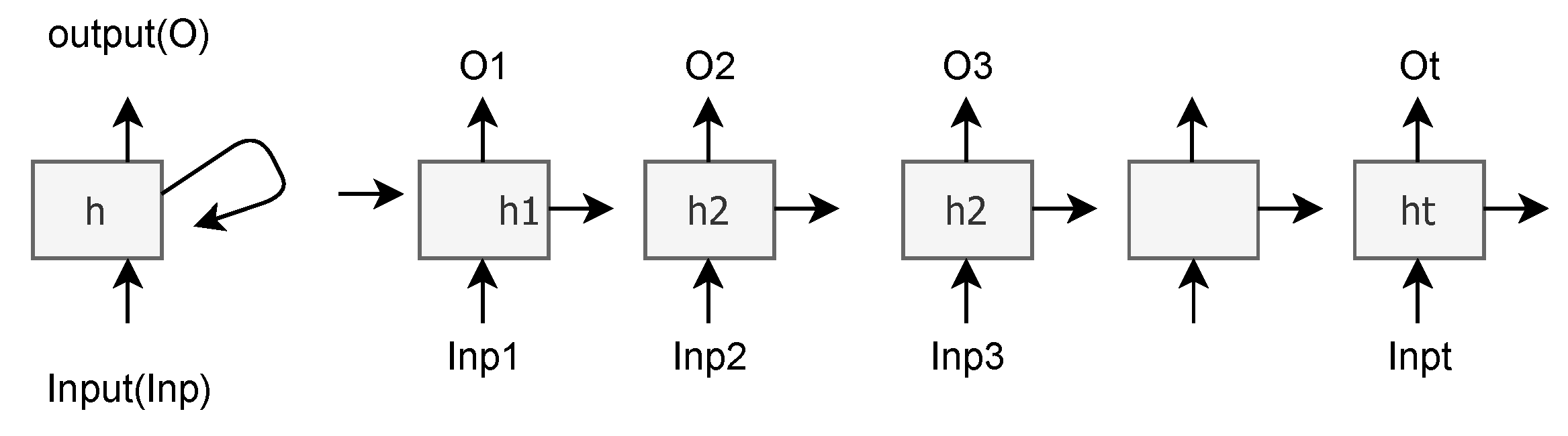
3.4.6. Predictive Model: Long Short-Term Memory (LSTM) Architecture

LSTM is a widely used artificial recurrent neural network (RNN) model to deal with sequential data. Since LSTM process the single data point and the sequential data points, it is efficient to train sequential data using LSTM. Some examples of sequential data points are text dataset, time-series dataset, voice dataset and video dataset. Sequential data maintains long-term dependencies, whereas LSTM is capable of learning long-term dependencies. LSTM is a modified version of RNN and RNN is capable of remembering previous data points. The basic architecture of LSTM is followed by the RNN model. An RNN architecture consists of three layers: input layer, hidden layer, and output layer [59,60]. The fundamental state (current state) of RNN architecture is as follows:

$$h_t=f(h_{t-1},x_t;\theta )$$

(9)

Here, $h_t$ refers to the current hidden state, f refers to the function of the previous hidden state $h_{t-1}$ and the current input $x_t$, $\theta$ refers to the parameters of that function.

The primary mechanism of an RNN architecture is that the hidden layer’s input is the current input and output derived from the earlier hidden state. Therefore, the hidden layer works as conditional neural memory and remembers the sequential data. The process is shown in a textual format and in Figure 1:

(Input + Previous_Hidden_output) –> Hidden –> Output

The drawback of the RNN architecture is that it forgets the necessary data when a very large dataset is used. The nature of time-series data is that the current data depends on the previous data. Hence, time-series data has long-term dependency over time. The LSTM model proposed by Hochreiter Long [61] is an improved version of RNN that can memorize the long-term dependency data by forgetting the unnecessary data and memorizing the necessary data at every updation step of gradient descent [62]. LSTM architecture comprises of four parts: a cell, an input gate, an output gate, and a forget cell [32]. The forget cell forgets the unnecessary data and remembers only the necessary data. The forget gate is responsible for deciding which information should be discarded based on the state h(t − 1) and input x(t) at the state c(t − 1). The forget gate’s sigmoid function keeps all 1s and discards all 0s between 0 and 1 values at each cell state. The value ‘1’ is considered as the necessary value, and ‘0’ is considered as the unnecessary value [14,61,63,64]. The equation of the forget gate state is as follows:

$$f_t=\sigma (W_f.[h_{t-1},x_t]+b_f)$$

(10)

where $f_t$ refers to the current forget state, $\sigma$ refers to the sigmoid activation function, $W_f$ refers to the weights of the forget gate, $h_{t-1}$ refers to the output from the previous hidden state, $x_t$ refers to current input and $b_f$ refers to the bias of the forget gate function.

After forgetting the unnecessary value, new values need to be updated in the cell state. The process has three parts:

• A sigmoid layer called the “input gate layer” decides which values to update.
• A tanh layer creates a vector of new candidate values to add to the state.
• Combination of step 1 and 2 creates an update to the state.

The sigmoid layer state’s equation is:

$$i_t=\sigma (W_i.[h_{t-1},x_t]+b_i)$$

(11)

Sigmoid layer from Equation (11) decides which value should be updated; tanh layer from Equation (12) creates a vector of new candidates for creating a new value to the state $C\left(t\right)$.

The tanh layer’s state equation is:

$$\tilde{C}\left(t\right)=tanh(W_c.[h_{t-1},x_t]+b_C)$$

(12)

The updation of the new cell at state $C\left(t\right)$ occurs by adding $\tilde{C}\left(t\right)\ast i_t$ with $C_{t-1}\ast f_t$. The updation state’s equation is:

$$C_t=C_{t-1}\ast f_t+\tilde{C}\left(t\right)\ast i_t$$

(13)

Finally, the output is filtered out by a sigmoid Equation (14) and a tanh Equation (15) function to decide which output needs to be kept.

$$O_t=\sigma (W_o.[h_{t-1},x_t]+b_o)$$

(14)

$$h_t=O_t\ast tanh\left(C_t\right)$$

(15)

where $h_t$ provides the output values for the next hidden layer’s input.

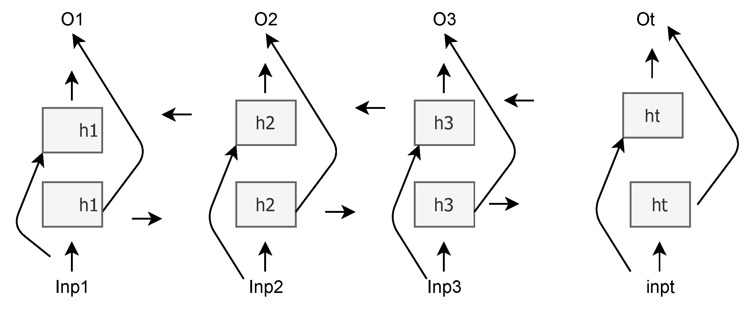
3.4.7. Predictive Model: BiLSTM Architecture

BiLSTM is almost the same as LSTM, except that it allows both forward and backward propagation. The BiLSTM model was first proposed by GRAVES [65]. LSTM does only forward propagation. BiLSTM’s architecture learns both from past-to-future data as well as future-to-past data. This concept makes the architecture more stable as it does not rely only on past data. Hence, BiLSTM seems to perform relatively better than LSTM. The structure of the bidirectional LSTM is shown in Figure 2. The backward propagation layer is mainly a reverse layer of forwarding LSTM. The hidden layer synthesizes both forward and backward information [66]. Hence, the reverse layer of LSTM is calculated as “the reverse direction of forward direction”. The BiLSTM network calculation formula is:

The formulation [66] of backward propagation is as follows:

$$h_f=f(w_{f1}{x}_t+w_{f2}{h}_{t-1})$$

(16)

$$h_b=f(w_{b1}{x}_t+w_{b2}{h}_{t+1})$$

(17)

where $h_f$ is the forward layer output, $h_b$ is the reverse layer output.

The hidden layer’s final output is given below:

$$O_i=g(w_{o1}\ast h_f+w_{o2}\ast h_b)$$

(18)

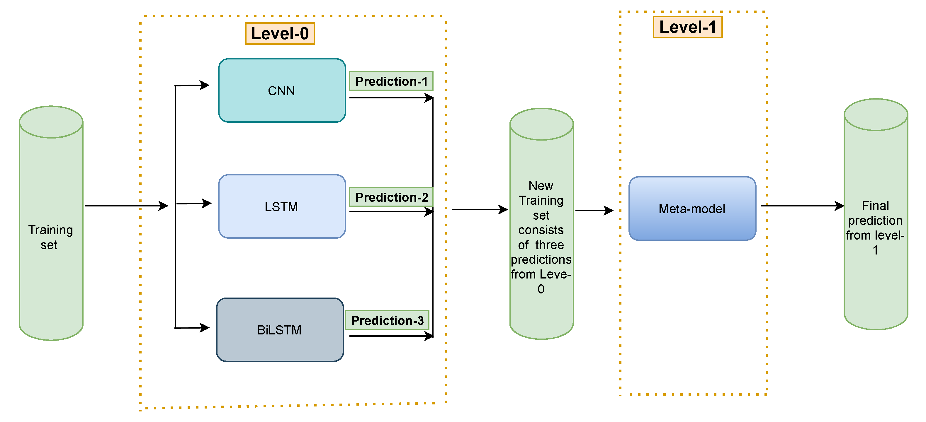
3.5. Proposed Model: Stacking Ensemble Neural Network Architecture

We have developed our proposed model using the stacking ensemble learning strategy. We have considered heterogeneous weak learners for the base models and linear regression for the meta-learner to build our proposed model. CNN, LSTM and BiLSTM models are used for creating the base models. We used the parameter “volatility”to feed into the architecture.

The proposed model’s data separation process is not the same as the process used in machine learning and deep learning techniques. The data is separated into three parts: 60 percent for training, 10 percent for validation and 30 percent for testing.

This change is necessary to avoid the overfitting tendency during the meta-learner training phase. Since the predicted dataset from the Level-0 is already a probability of expected values, the meta-learner has a high chance of giving the exact probabilities as Level-0. The combination of the validation dataset and the predicted dataset is used to train the final model (meta-learner) to avoid overfitting issues. The prediction from Level-1 is the final output. The stacking ensemble takes predicted results from multiple models and uses the predicted results for a final model (meta-learner) which is the output of the stacking ensemble model.

The problem with the traditional stacking ensemble method is that the same multiple models are used for the base model, which gives similar predictions. If the base model performs poorly on the dataset, there is a high chance of obtaining an overall poor result. However, the single neural network model has a bias and variance tendency towards the dataset. So, we go for dissimilar models for creating the base model.

Figure 3 illustrates a high-level schematic representation of the proposed stacking ensemble of neural network model.

As shown in Figure 3, the architecture has two parts: $Level-0$ and $Level-1$.

$Level-0$ is built with CNN, LSTM and BiLSTM model. The three submodels learn the data pattern and give three predictions parallelly. Each of the models used in $Level-0$ has an equal contribution to the whole model.

$Level-1$ is built with one linear regression; this is also called the meta-learner of the architecture. The predicted outputs from Level 0 are used as input for the meta-learner in Level-1. The meta learner best guesses the final outputs based on the predicted outputs from Level-0. The meta learner refers to a model that can rapidly learn a new pattern or adapt to new datasets with a few training examples. The linear regression works as a meta learner; the meta learner learns the pattern that has already been learned from three different models. Hence, the model can learn utterly new data very well and can provide a satisfactory result.

4. Result and Discussion

Our proposed model worked best on twenty different companies’ datasets of a frontier market. Using our dataset, we have trained four machine learning ensemble models, such as Random Forest, AdaBoost, GradientBoosting, Xgboost, and ML stacking ensemble, then three deep learning models such as CNN, LSTM, and BiLSTM, and finally, with our proposed stacking ensemble neural network model. The results in

Table 2. Experiment results obtained from 20 different companies’ stock price datasets of a frontier market using deep learning models such as CNN, LSTM, BiLSTM and our proposed STacking Ensemble of Neural Network model.

Dataset	Deep Learning Models	RMSE	MAE
ABBANK	CNN	3.6829	3.4811
	LSTM	3.8222	3.7760
	BiLSTM	3.9660	3.9122
	Proposed Stacking Ensemble of Neural Network	0.6766	0.5116
ACIBANK	CNN	2.3866	1.8764
	LSTM	1.2314	0.9824
	BiLSTM	0.2280	0.1931
	Proposed Stacking Ensemble of Neural Network	1.1880	0.8805
APEXFOOT	CNN	5.4682	5.3320
	LSTM	4.7450	4.5975
	BiLSTM	1.3357	1.0584
	Proposed Stacking Ensemble of Neural Network	1.0634	0.9504
BANKASIA	CNN	0.6713	0.5675
	LSTM	0.4191	0.3472
	BiLSTM	0.4956	6.8461
	Proposed Stacking Ensemble of Neural Network	0.8139	0.6806
BATASHOE	CNN	6.3256	6.0763
	LSTM	7.7107	7.5957
	BiLSTM	1.5567	1.3306
	Proposed Stacking Ensemble of Neural Network	0.9859	0.7908
BERGERPBL	CNN	5.4822	5.4256
	LSTM	5.4605	5.3972
	BiLSTM	4.4781	4.4417
	Proposed Stacking Ensemble of Neural Network	0.4721	0.3812
BEXIMCO	CNN	5.8887	5.8245
	LSTM	5.3503	5.3172
	BiLSTM	2.5656	2.5383
	Proposed Stacking Ensemble of Neural Network	0.6300	0.4795
BRACBANK	CNN	4.3199	3.7514
	LSTM	2.7113	2.3612
	BiLSTM	4.0452	3.3964
	Proposed Stacking Ensemble of Neural Network	2.1705	2.4467
CITYBANK	CNN	3.2923	3.1774
	LSTM	1.8324	1.7528
	BiLSTM	2.7964	2.7133
	Proposed Stacking Ensemble of Neural Network	0.7283	0.6993
DESCO	CNN	1.0141	0.8770
	LSTM	0.9895	0.8442
	BiLSTM	0.7367	0.5795
	Proposed Stacking Ensemble of Neural Network	0.8349	0.8349
DHAKABANK	CNN	1.5500	0.8770
	LSTM	1.0917	1.0176
	BiLSTM	1.6444	1.4745
	Proposed Stacking Ensemble of Neural Network	0.5206	0.5206
DUTCHBANGLABANK	CNN	11.5777	11.4175
	LSTM	15.2332	15.1668
	BiLSTM	10.1262	10.0926
	Proposed Stacking Ensemble of Neural Network	1.0317	0.9021
EXIMBANK	CNN	0.8822	0.7254
	LSTM	1.04872	0.8899
	BiLSTM	0.4895	0.3822
	Proposed Stacking Ensemble of Neural Network	0.4631	0.4093
FUWANGFOOD	CNN	3.6536	2.7259
	LSTM	4.4977	3.5727
	BiLSTM	2.2982	1.8985
	Proposed Stacking Ensemble of Neural Network	2.5696	2.444
GP	CNN	1.6824	1.4521
	LSTM	0.9660	0.7848
	BiLSTM	1.0760	0.9343
	Proposed Stacking Ensemble of Neural Network	0.5970	0.4611
IBNSINA	CNN	1.4132	1.2915
	LSTM	1.6709	1.5288
	BiLSTM	1.0107	0.8399
	Stacking Neural Network Ensemble	0.9153	0.9659
IFIC	CNN	1.1520	0.9446
	LSTM	1.81234	1.5902
	BiLSTM	1.8714	1.8041
	Proposed Stacking Ensemble of Neural Network	0.3626	0.3682
JAMUNABANK	CNN	1.0167	0.8089
	LSTM	0.4649	0.3752
	BiLSTM	0.7879	0.6579
	Proposed Stacking Ensemble of Neural Network	0.5614	0.5526
KEYACOSMET	CNN	6.8706	6.6129
	LSTM	5.8391	5.7513
	BiLSTM	8.4249	8.3693
	Proposed Stacking Ensemble of Neural Network	1.0614	0.9095
UTTARABANK	CNN	1.3121	1.0543
	LSTM	0.9504	0.7705
	BiLSTM	0.6997	0.5853
	Proposed Stacking Ensemble of Neural Network	0.6741	0.6611

have shown that the machine learning ensemble models have provided substantial RMSE errors. We have achieved the highest RMSE error of 15.489 and the highest MAE error value of 15.416 using the machine learning models. The machine learning models’ error rates are higher than the neural network and our proposed models’ error rates. CNN works well on some of the data patterns, but not all. For instance, companies such as ACIBANK, BANKASIA, DESCO, DHAKABANK, EXIMBANK, GP, IBNSINA, IFIC, JAMUNABANK and UTTARABANK have lower RMSE error percentages of 2.3866, 0.6713, 1.5500, 0.8770, 0.8822, 1.6824, 1.4132, 1.1520, 1.0167, and 1.3121, respectively. On the other hand, companies such as ABBANK, APEXFOOD, BATASHOE, BERGERPBL, BEXIMCO, BRACBANK, CITYBANK, DUTCHBANGLABANK, FUWANGFOOD and KEYACOSMET have higher RMSE error percentages of 3.6829, 5.4682, 6.3256, 5.4822, 5.8887, 4.3199, 3.2923, 11.5777, 3.6536, and 6.8706, respectively. LSTM and BiLSTM models also show inconsistent results over the datasets. LSTM performed better on ACIBANK, BANKASIA, BRACKBANK, CITYBANK, DESCO, DHAKABANK, EXIMBANK, GP, IBNSINA, IFIC, JAMUNABANK and UTTARABANK with an error rate of 1.2314, 0.4191, 2.7113, 1.8324, 0.9894, 1.0917, 1.04872, 0.9660, 1.6709, 1.8123, 0.4649 and 0.9504, respectively, and performed poorly on ABBANK, APEXFOOT, BATASHOE, BERGERPBL, BEXIMCO, DUTCHBANGLABANK, FUWANGFOOD and KEYACOSMET with RMSE error rates of 3.8222, 4.7450, 7.7107, 5.4605, 5.3503, 15.2332, 4.4977, and 5.8391. BiLSTM provides satisfactory results on ACIBANK, APEXFOOT, BANKASIA, BATASHOE, BEXIMCO, CITYBANK, DESCO, DHAKABANK, EXIMBANK, FUWANGFOOD, GP, IBNSINA, IFIC, JAMUNABANK, and UATTARABANK with the RMSE error rates of 0.2280, 1.3357, 0.4956, 1.5567, 2.5656, 2.7964, 0.7367, 1.6444, 0.4895, 2.2982, 1.0760, 1.0107, 1.8714, 0.7879 and 0.6997, respectively, and unsatisfactory result on ABBANK, BERGERPBL, BRACBANK, DUTCHBANGLABANK and KEYACOSMET with RMSE error rates of 3.9660, 4.4781, 4.0452, 10.1262 and 8.4249, respectively. These results show that BiLSTM performs comparatively better than CNN and LSTM. The main problem is that none of the traditional models confirm that they can precisely predict every dataset. The randomness in the result proves that we cannot rely on those models. However, our proposed model provides a satisfactory result for every company: ABBANK, ACIBANK, APEXFOOT, BANKASIA, BATASHOE, BERGERPBL, BEXIMCO, BRACBANK, CITYBANK, DESCO, DHAKABANK, DUTCHBANGLABANK, EXIMBANK, FUWANGFOOD, GP, IBNSINA, IFIC, JAMUNABANK, KEYACOSMET and UTTARABANK had RMSE error rates of 0.6766, 1.1880, 1.0634, 0.8139, 0.9859, 0.4721, 0.6300, 2.1705, 0.7283, 0.8349, 0.5206, 1.0317, 1.0317, 2.5696, 2.5696, 0.9153, 0.3626, 0.5614, 1.0614 and 0.6741, respectively, which clearly evidence that it maintains consistent results on every dataset. Moreover, our model can maintain high accuracy on multiple data patterns as we have achieved the RMSE and MAE error values between $0<result<3$ for all the datasets. Our proposed model has shown a consistent low error rate and outstanding accuracy as the RMSE value has remained below 2.

Table 3. Experiment results obtained from 20 different companies’ stock price datasets of a frontier market using machine learning models such as RandomForest, AdaBoost, GradientBoosting and ML stacking Ensemble Learning.

Dataset	Machine Learning Models	RMSE	MAE
ABBANK	ML ensemble method (RandomForest)	4.3384	4.2509
	ML ensemble method (AdaBoost)	6.1229	6.0434
	ML ensemble method (GradientBoosting)	6.9083	6.8461
	ML Stacking Ensemble Learning	5.1710	4.8450
ACIBANK	ML ensemble method (RandomForest)	2.3326	1.6824
	ML ensemble method (AdaBoost)	2.7053	2.0491
	ML ensemble method (GradientBoosting)	2.4149	1.8078
	ML Stacking Ensemble Learning	1.9230	1.6032
APEXFOOT	ML ensemble method (Randomforest)	6.6466	6.4764
	ML ensemble method (AdaBoost)	7.3927	7.2382
	ML ensemble method (GradientBoosting)	7.6668	7.526
	ML Stacking Ensemble Learning	5.2078	5.0352
BANKASIA	ML ensemble method (RandomForest)	0.4049	0.3000
	ML ensemble method (AdaBoost)	0.4208	0.2945
	ML ensemble method (GradientBoosting)	0.4052	0.2987
	ML Stacking Ensemble Learning	0.6428	0.4658
BATASHOE	ML ensemble method (RandomForest)	6.2606	5.9338
	ML ensemble method (AdaBoost)	7.1886	6.9948
	ML ensemble method (GradientBoosting)	6.0615	5.7666
	ML Stacking Ensemble Learning	5.7256	5.6674
BERGERPBL	ML ensemble method (RandomForest)	5.3535	5.2818
	ML ensemble method (AdaBoost)	7.8242	7.7765
	ML ensemble method (GradientBoosting)	6.6984	7.0529
	ML Stacking Ensemble Learning	4.9378	4.8600
BEXIMCO	ML ensemble method (RandomForest)	6.4896	6.3802
	ML ensemble method (AdaBoost)	7.1802	7.0570
	ML ensemble method (GradientBoosting)	7.1802	7.5636
	ML Stacking Ensemble Learning	9.5758	9.5000
BRACBANK	ML ensemble method (Randomforest)	5.8722	4.4277
	ML ensemble method (AdaBoost)	6.3241	4.8102
	ML ensemble method (GradientBoosting)	7.1432	5.7192
	ML Stacking Ensemble Learning	6.5281	5.6115
CITYBANK	ML ensemble method (Randomforest)	3.6603	3.5544
	ML ensemble method (Adaboost)	5.1566	5.0716
	ML ensemble method (GradientBoosting)	4.5469	4.4633
	ML Stacking Ensemble Learning	3.6076	3.5365
DESCO	ML ensemble method (Randomforest)	1.0350	0.8394
	ML ensemble method (Adaboost)	1.6060	1.3092
	ML ensemble method (GradientBoosting)	1.1690	0.9720
	ML Stacking Ensemble Learning	0.9726	0.8290
DHAKABANK	ML ensemble method (RandomForest)	1.4607	1.2543
	ML ensemble method (AdaBoost)	1.7555	1.6016
	ML ensemble method (GradientBoosting)	1.6657	1.4554
	ML Stacking Ensemble Learning	1.6992	1.5735
DUTCHBANGLABANK	ML ensemble method (RandomForest)	15.4895	15.4166
	ML ensemble method (AdaBoost)	18.8228	18.7540
	ML ensemble method (GradientBoosting)	14.9011	14.8032
	ML Stacking Ensemble Learning	20.4852	20.4260
Eximbank	ML ensemble method (Randomforest)	0.9836	0.8807
	ML ensemble method (Adaboost)	1.4827	1.3170
	ML ensemble method (GradientBoosting)	1.2541	1.0899
	ML Stacking Ensemble Learning	0.7287	0.6072
Fuwangfood	ML ensemble method (RandomForest)	7.3138	6.1929
	ML ensemble method (AdaBoost)	7.5585	6.2670
	ML ensemble method (GradientBoosting)	9.7713	8.6078
	ML Stacking Ensemble Learning	5.2664	4.5548
IBNSINA	ML ensemble method (RandomForest)	1.3931	1.1716
	ML ensemble method (AdaBoost)	1.5116	1.2887
	ML ensemble method (GradientBoosting)	1.4613	1.2196
	ML Stacking Ensemble Learning	1.2653	1.0263
IFIC	ML ensemble method (Randomforest)	3.5166	3.4134
	ML ensemble method (AdaBoost)	3.8412	3.7434
	ML ensemble method (GradientBoosting)	4.2209	4.0965
	ML Stacking Ensemble Learning	2.9332	2.8153
JAMUNABANK	ML ensemble method (RandomForest)	0.3725	0.2716
	ML ensemble method (AdaBoost)	0.4013	0.2725
	ML ensemble method (GradientBoosting)	0.5965	0.4986
	ML Stacking Ensemble Learning	0.5364	0.4164
KEYACOSMET	ML ensemble method (RandomForest)	6.7334	6.4327
	ML ensemble method (AdaBoost)	7.7225	7.4159
	ML ensemble method (GradientBoosting)	8.1252	7.5307
	ML Stacking Ensemble Learning	9.0140	8.8783
UTTARABANK	ML ensemble method (RandomForest)	0.9987	0.6482
	ML ensemble method (AdaBoost)	1.0256	0.6621
	ML ensemble method (GradientBoosting)	1.0327	0.6583
	ML stacking Ensemble Learning	0.9832	0.7307

provides the representation of RMSE and MAE error values obtained from 20 different datasets of a frontier market using machine learning ensemble models such as RandomForest, AdaBoost, GradientBoosting and ML stacking Ensemble Learning.

Table 2 provides the representation of RMSE and MAE error values obtained from twenty different datasets of a frontier market using deep learning models such as CNN, LSTM and Bi-LSTM and our proposed stacking ensemle of neural network model.

Earlier, several ensemble learning methods have been proposed in the literature for analyzing the time series data. X. Qiu et al. [19] developed an ensemble learning model with a different number of epochs using the same feedforward back-propagation neural networks (FNN) model and experimented on electricity load demand datasets such as Mackey–Glass, NSW, SA, TAS, CART, FAD and CH. They compared their proposed model’s result with traditional machine learning and deep learning models such as support vector regression (SVR), feedforward neural network (FNN), deep belief network (DBN) and ensemble feedforward neural network (ENN). The RMSE results shown in

Table 4. RMSE Results derived from existing work.

Dataset Name	SVR	FNN	DBN	ENN	Proposed
Mackey-Glass	0.0024	0.002	0.0018	0.0226	0.0015
NSW	74.3053	95.8105	90.2061	78.6394	72.2545
SA	44.6742	38.8585	35.9375	34.9473	30.5989
TAS	20.1068	19.7952	19.9187	19.9034	19.7580
CART	0.0406	0.0420	0.0412	0.0428	0.0403
FAD	0.0339	0.0349	0.0320	0.0315	0.0313
CH	0.1637	0.1803	0.1773	0.1615	0.1508

confirm that their proposed model works better than the aforementioned traditional models. However, the results they received show no significant difference. Therefore, a small difference does not create any novelty in this research area.

S. Li et al. [22] developed a hybrid convolutional neural network for environmental sound recognition. They stacked the model with two models, MelNet [67] and RawNet [68]. Each of the models contains five convolutional neural networks and a fully connected layer. They used the accuracy evaluation metric and evaluated this model on three datasets such as ESC-10, ESC-50 and Urbansound8k, which are audio signal datasets. They achieved an accuracy of 91.4 percent for MelNet, which is 9.9 percent and 4.5 percent higher than the accuracy (81.5 percent) of previous work Piczak’s [69]. Finally, they evaluated the algorithms on the Urbansound8k dataset. The accuracy of MelNet is 90.2 percent, which is also higher than the 73.7 percent accuracy of Piczak [69] and the 79 percent of Salamon and Bello [70]. The concept of their developed model is similar but not identical to ours. The evaluation metric and dataset differ significantly from the regression problem metric and time series dataset.

Carta et al. [20] developed a stacking ensemble learning with hundreds of deep learning decisions, provided by a large number of CNNs trained with historical market data encoded into GAF images and used them as input for a reinforcement meta learner classifier. Finally, they use meta learner for final prediction. Though they have improved the result, the approach they have followed is basically for the classification problem.

The problems with the existing models are showing biased results on a particular dataset and weak learners. Varying only the parameters is not a good approach since each parameter can work differently on a different dataset. Moreover, single models are not capable of working well on multiple datasets. Therefore, we have developed our model by taking account of those issues. We have developed a completely new deep learning model for the regression and classification problem and experimented on a time-series dataset that falls under the regression problem. Since our developed model has not been reported yet, we have shown comparative analysis with the existing models and found that our model significantly reduces the value of error metrics.

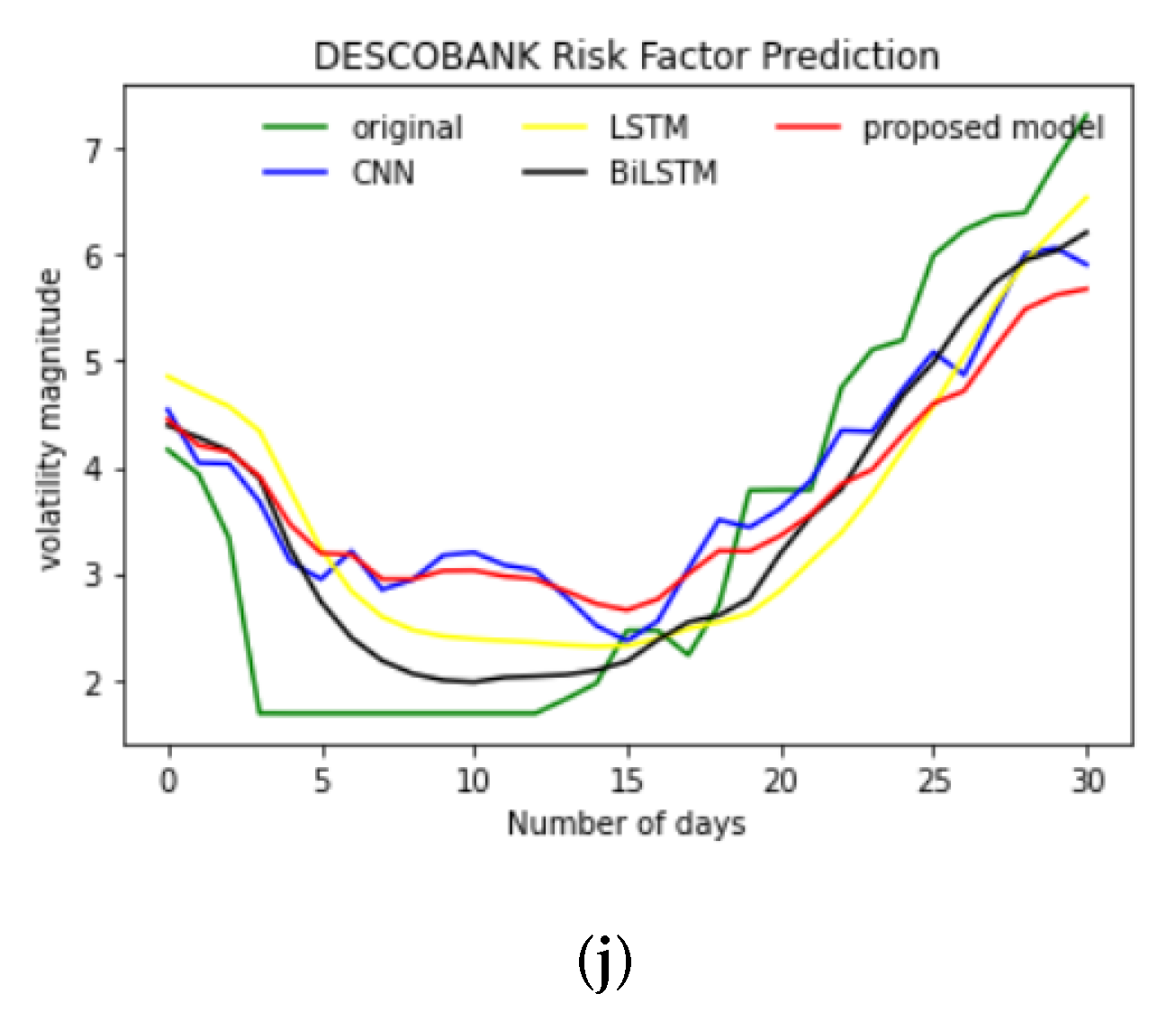
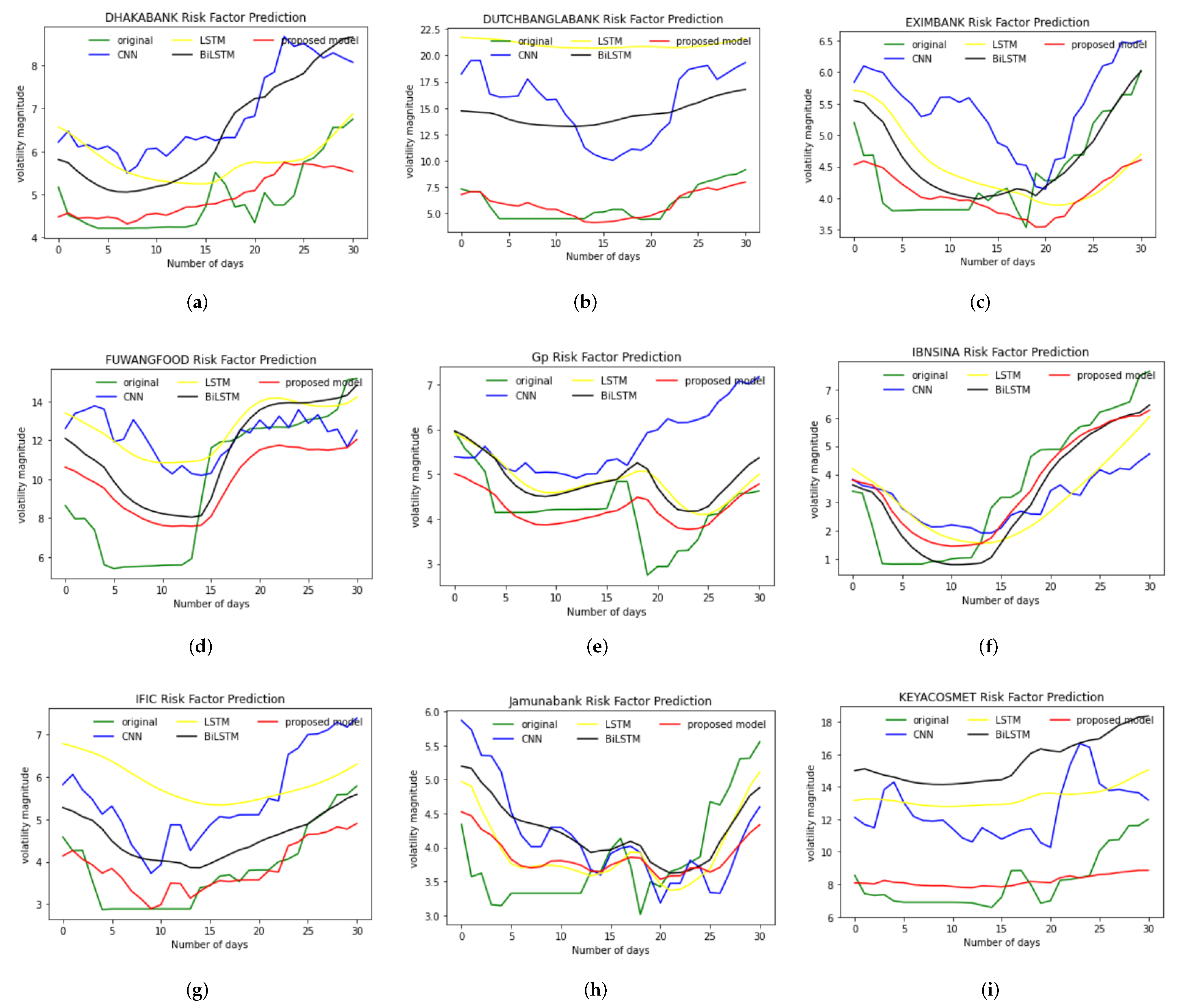
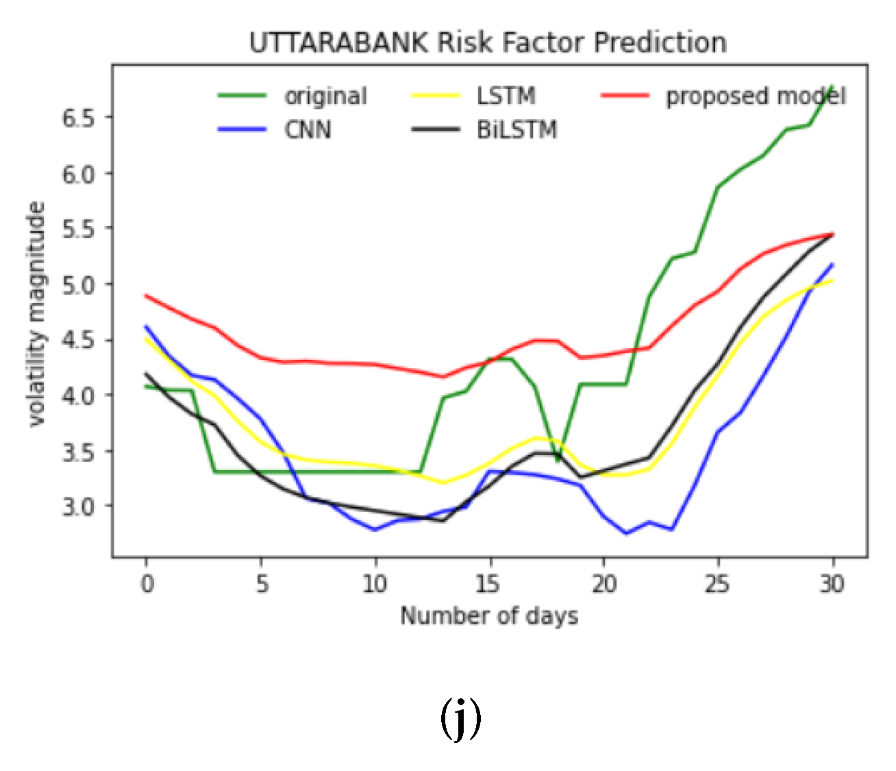
4.1. Predicted Results

The predicted results of twenty selected datasets of Bangladesh frontier market are shown in Figure 4 and Figure 5. The CNN, LSTM, BILSTM and proposed models’ results are individually plotted on the test dataset.

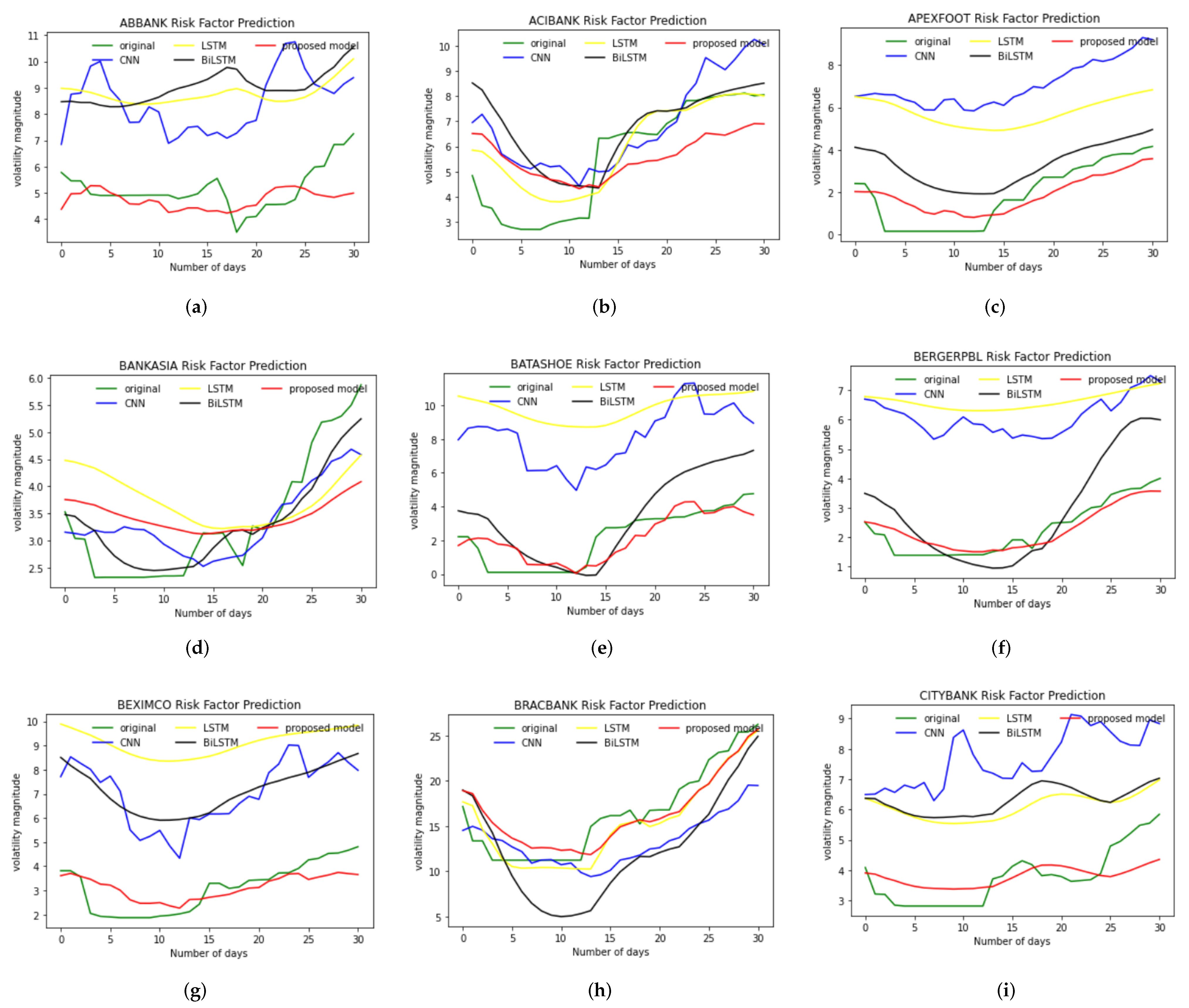
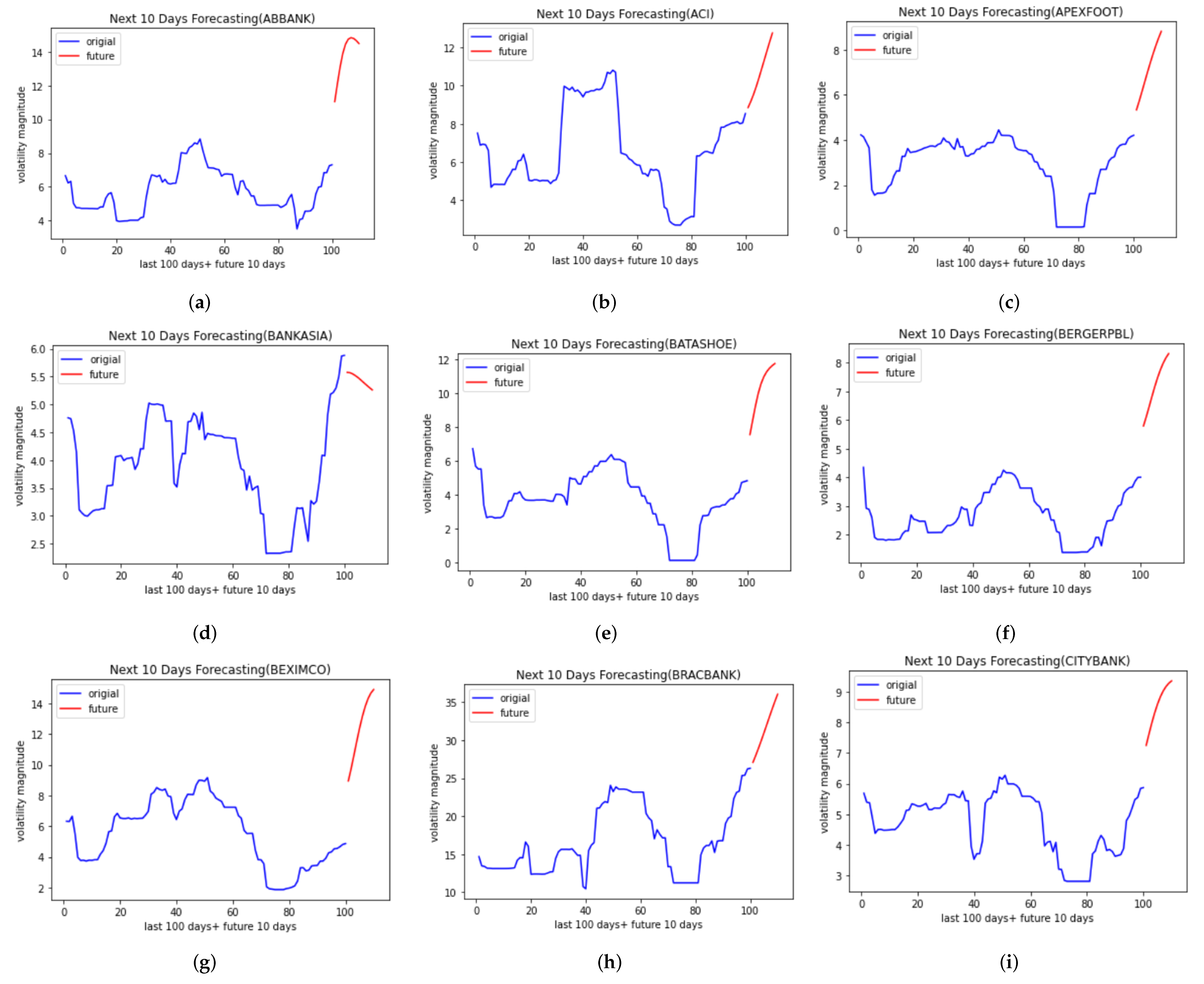
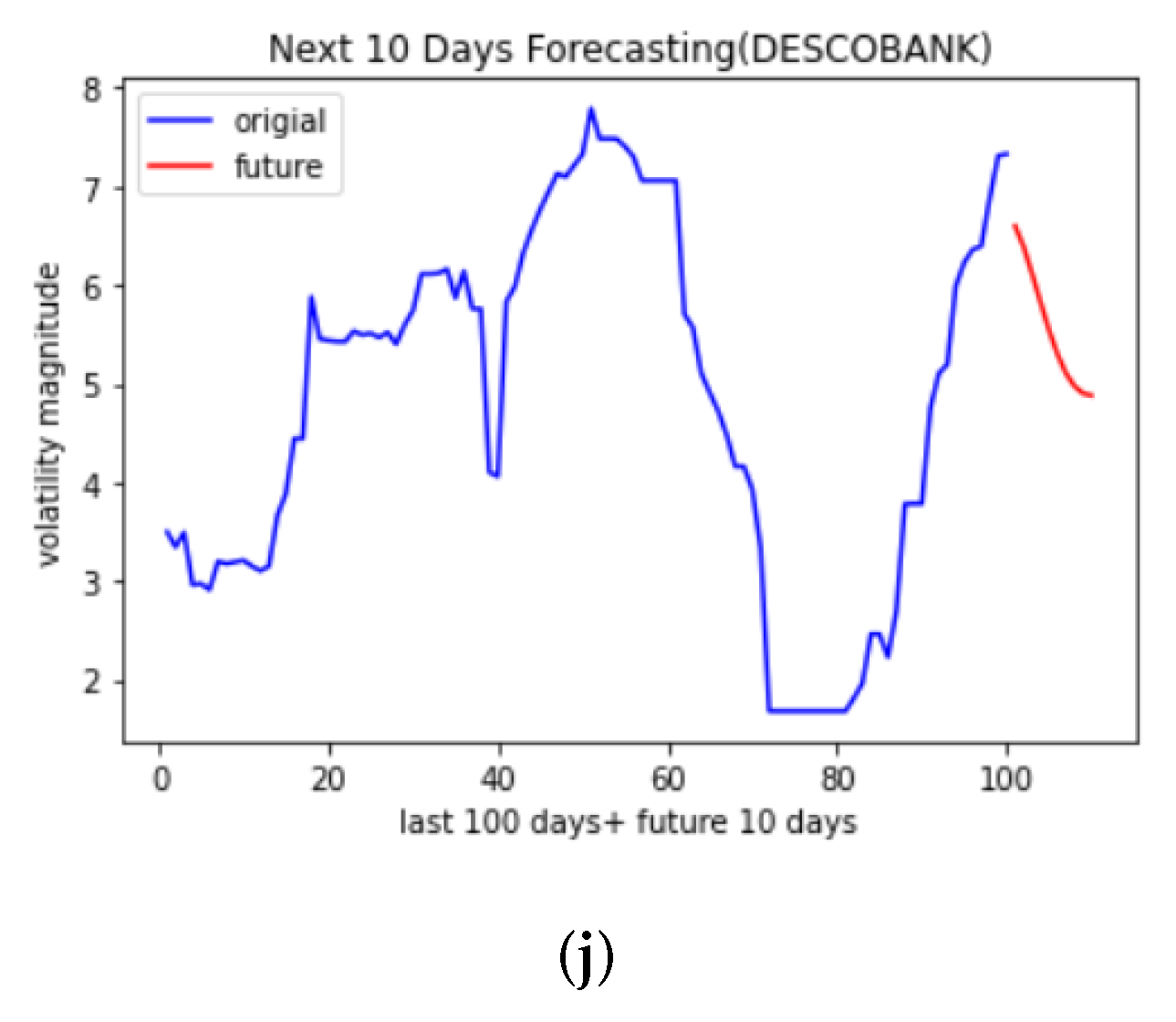
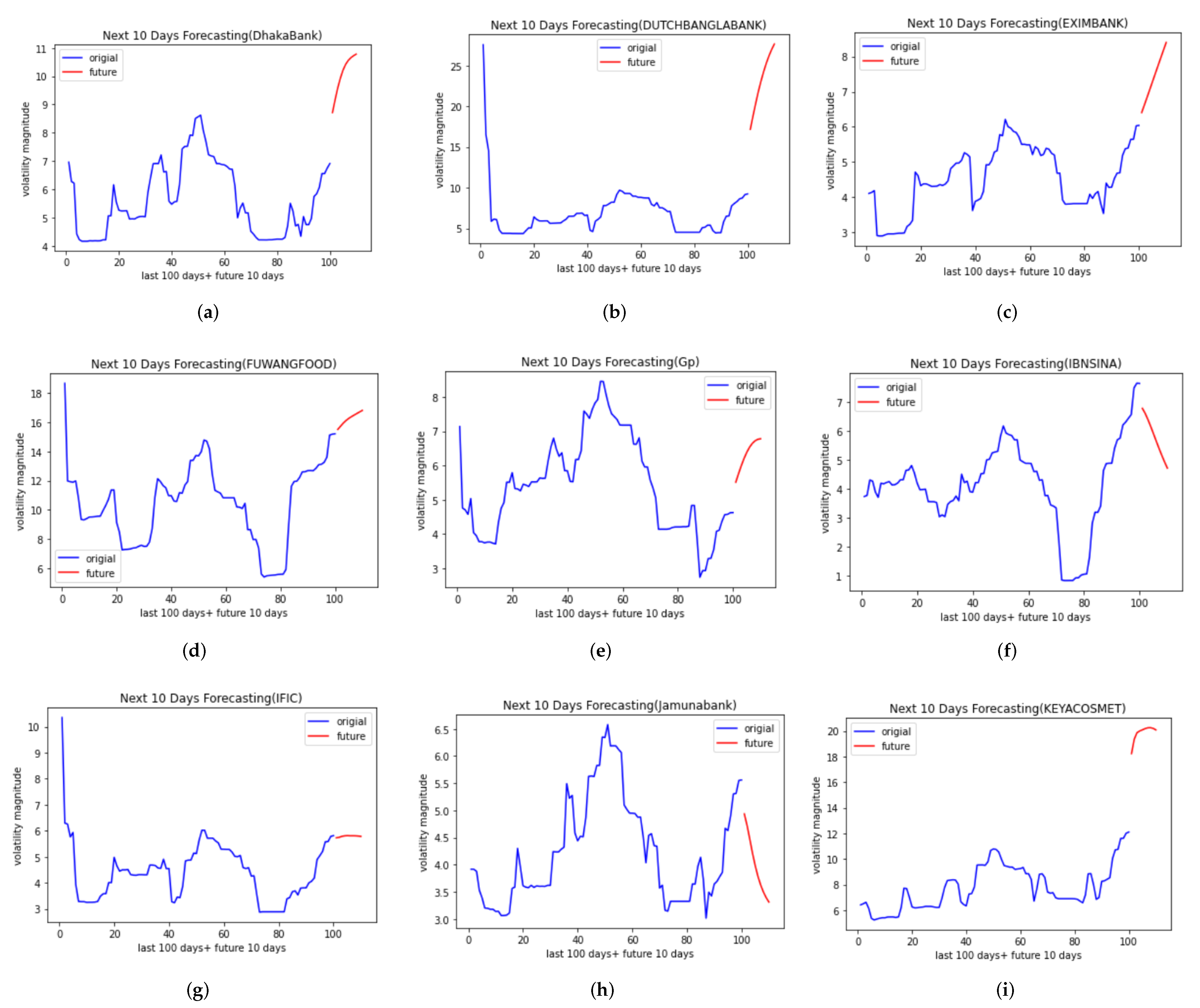
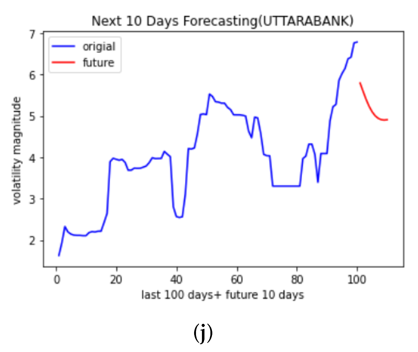
4.2. Forecasting Results

The forecasting results for 20 frontier market datasets are shown in Figure 6 and Figure 7. Future 10 days of risk factor is forecasted using our proposed model.

5. Conclusions

Our paper has shown a new approach for predicting the risk factor of any company in a frontier market. The approach is useful for a frontier market as it shows both the processes of finding the missing parameter named “volatility”, which does not exist in this market, and predicting the risk factor using the estimated “volatility” parameter. The prediction process is helpful for investors who invest money in this market as well as in other frontier markets. The volatility prediction may help investors to increase their profit since the high and low volatility indicate a significant fluctuation from the regular prices. The investors can obtain an idea of the future risk of the frontier market that will allow them to invest carefully. The machine learning models are capable of capturing the pattern of the risk factor depending on the parameter “volatility”. After capturing the pattern, the model can give future predictions. It should be noted that the future prediction values can be reliable only if the model performs well. The measurement of the correctness of a model can be evaluated with the help of evaluation metrics. In our paper, we have used RMSE and MSE metrics to evaluate all the models. The metric evaluation result shows that our proposed model performs best among all the machine learning models, which is not more than RMSE and MAE values of 2.5696 and 2.444 percent, respectively. However, the traditional machine learning models give very high RMSE and MAE error rates, which are 20.4852 and 20.4260 percent, respectively. The deep learning models also provide a high rate of RMSE and MAWE value such as the traditional machine learning models, e.g., 15.2332 and 15.1668 percent; for such cases, our proposed model reduces the error rate significantly and gives an error rate no more than the value of 3. Therefore, our model is capable of providing very high accuracy even if traditional models fail to do that. The reason for showing the poor result of the traditional machine learning models is that a single machine learning or deep learning model has the tendency of bias and variance issues. We have tried to overcome the issues and achieved a satisfactory result, which concludes that our proposed model can be useful for predicting the risk factor of the frontier market with high accuracy. Since the topic of predicting the risk factor of the frontier market is fully undiscovered, we have tried to contribute in this area by showing the process of calculating the “volatility” parameter, by making a comparative work using several machine learning and deep learning models and by developing a new stacking ensemble of neural network model. We believe that by following our work, future researchers might be motivated to contribute in this area, which will help the area to be considered as a big and an important part of future investigations.

References

1. Gomes, M.; Chaibi, A. Volatility spillovers between oil prices and stock returns: A focus on frontier markets. J. Appl. Bus. Res. 2014, 30, 18. [Google Scholar] [CrossRef]
2. Chowdhury, R.; Mahdy, M.; Alam, T.N.; Al Quaderi, G.D.; Rahman, M.A. Predicting the stock price of frontier markets using machine learning and modified Black–Scholes Option pricing model. Phys. A Stat. Mech. Appl. 2020, 555, 124444. [Google Scholar] [CrossRef]
3. Anghel, D.G. Predicting Intraday Prices in the Frontier Stock Market of Romania Using Machine Learning Algorithms. Int. J. Econ. Financ. Res. 2020, 6, 170–179. [Google Scholar] [CrossRef]
4. Lin, K.; Lin, Q.; Zhou, C.; Yao, J. Time series prediction based on linear regression and SVR. In Proceedings of the Third International Conference on Natural Computation (ICNC 2007), Haikou, China, 24–27 August 2007; IEEE: New York, NY, USA, 2007; Volume 1, pp. 688–691. [Google Scholar]
5. Kavitha, S.; Varuna, S.; Ramya, R. A comparative analysis on linear regression and support vector regression. In Proceedings of the 2016 Online International Conference on Green Engineering and Technologies (IC-GET), Virtual, 19 November 2016; IEEE: New York, NY, USA, 2016; pp. 1–5. [Google Scholar]
6. Johnsson, O. Predicting Stock Index Volatility Using Artificial Neural Networks: An Empirical Study of the OMXS30, FTSE100 & S&P/ASX200. Master’s Thesis, Lund University, Lund, Sweden, 2018. [Google Scholar]
7. Madge, S.; Bhatt, S. Predicting stock price direction using support vector machines. In Independent Work Report Spring; Princeton University: Princeton, NJ, USA, 2015; Volume 45. [Google Scholar]
8. Yoon, Y.; Swales, G. Predicting stock price performance: A neural network approach. In Proceedings of the Twenty-Fourth Annual Hawaii International Conference on System Sciences, Kauai, HI, USA, 8–11 January 1991; IEEE: New York, NY, USA, 1991; Volume 4, pp. 156–162. [Google Scholar]
9. Zhao, Y.; Li, J.; Yu, L. A deep learning ensemble approach for crude oil price forecasting. Energy Econ. 2017, 66, 9–16. [Google Scholar] [CrossRef]
10. Chen, Z.; Li, C.; Sun, W. Bitcoin price prediction using machine learning: An approach to sample dimension engineering. J. Comput. Appl. Math. 2020, 365, 112395. [Google Scholar] [CrossRef]
11. Andriopoulos, N.; Magklaras, A.; Birbas, A.; Papalexopoulos, A.; Valouxis, C.; Daskalaki, S.; Birbas, M.; Housos, E.; Papaioannou, G.P. Short Term Electric Load Forecasting Based on Data Transformation and Statistical Machine Learning. Appl. Sci. 2021, 11, 158. [Google Scholar] [CrossRef]
12. Selvin, S.; Vinayakumar, R.; Gopalakrishnan, E.; Menon, V.K.; Soman, K. Stock price prediction using LSTM, RNN and CNN-sliding window model. In Proceedings of the 2017 International Conference on Advances in Computing, Communications and Informatics (ICACCI), Udupi, India, 13–16 September 2017; IEEE: New York, NY, USA, 2017; pp. 1643–1647. [Google Scholar]
13. Patel, M.B.; Yalamalle, S.R. Stock price prediction using artificial neural network. Int. J. Innov. Res. Sci. Eng. Technol. 2014, 3, 13755–13762. [Google Scholar]
14. Liu, S.; Liao, G.; Ding, Y. Stock transaction prediction modeling and analysis based on LSTM. In Proceedings of the 2018 13th IEEE Conference on Industrial Electronics and Applications (ICIEA), Wuhan, China, 31 May–1 June 2018; IEEE: New York, NY, USA, 2018; pp. 2787–2790. [Google Scholar]
15. Siami-Namini, S.; Tavakoli, N.; Namin, A.S. The performance of LSTM and BiLSTM in forecasting time series. In Proceedings of the 2019 IEEE International Conference on Big Data (Big Data), Los Angeles, CA, USA, 9–12 December 2019; IEEE: New York, NY, USA, 2019; pp. 3285–3292. [Google Scholar]
16. Elliot, A.; Hsu, C.H. Time Series Prediction: Predicting Stock Price. arXiv 2017, arXiv:1710.05751. [Google Scholar]
17. Elsayed, S.; Thyssens, D.; Rashed, A.; Schmidt-Thieme, L.; Jomaa, H.S. Do We Really Need Deep Learning Models for Time Series Forecasting? arXiv 2021, arXiv:2101.02118. [Google Scholar]
18. Luong, C.; Dokuchaev, N. Forecasting of realised volatility with the random forests algorithm. J. Risk Financ. Manag. 2018, 11, 61. [Google Scholar] [CrossRef]
19. Qiu, X.; Zhang, L.; Ren, Y.; Suganthan, P.N.; Amaratunga, G. Ensemble deep learning for regression and time series forecasting. In Proceedings of the 2014 IEEE Symposium on Computational Intelligence in Ensemble Learning (CIEL), Orlando, FL, USA, 9–12 December 2014; IEEE: New York, NY, USA, 2014; pp. 1–6. [Google Scholar]
20. Carta, S.; Corriga, A.; Ferreira, A.; Podda, A.S.; Recupero, D.R. A multi-layer and multi-ensemble stock trader using deep learning and deep reinforcement learning. Appl. Intell. 2021, 51, 889–905. [Google Scholar] [CrossRef]
21. Livieris, I.E.; Pintelas, E.; Stavroyiannis, S.; Pintelas, P. Ensemble deep learning models for forecasting cryptocurrency time-series. Algorithms 2020, 13, 121. [Google Scholar] [CrossRef]
22. Li, S.; Yao, Y.; Hu, J.; Liu, G.; Yao, X.; Hu, J. An ensemble stacked convolutional neural network model for environmental event sound recognition. Appl. Sci. 2018, 8, 1152. [Google Scholar] [CrossRef] [Green Version]
23. Dey, S.; Kumar, Y.; Saha, S.; Basak, S. Forecasting to Classification: Predicting the Direction of Stock Market Price Using Xtreme Gradient Boosting; PESIT South Campus: Bengaluru, India, 2016. [Google Scholar]
24. Albaity, M.S. Impact of the monetary policy instruments on Islamic stock market index return. Econ. Discuss. Pap. 2011. [Google Scholar] [CrossRef]
25. Selemela, S.M.; Ferreira, S.; Mokatsanyane, D. Analysing Volatility during Extreme Market Events Using the Mid Cap Share Index. Economica 2021, 17, 229–249. [Google Scholar]
26. Ederington, L.H.; Guan, W. Measuring historical volatility. J. Appl. Financ. 2006, 16, 10. [Google Scholar]
27. Poon, S.H.; Granger, C. Practical issues in forecasting volatility. Financ. Anal. J. 2005, 61, 45–56. [Google Scholar] [CrossRef]
28. Botchkarev, A. Performance metrics (error measures) in machine learning regression, forecasting and prognostics: Properties and typology. arXiv 2018, arXiv:1809.03006. [Google Scholar]
29. Garosi, Y.; Sheklabadi, M.; Conoscenti, C.; Pourghasemi, H.R.; Van Oost, K. Assessing the performance of GIS-based machine learning models with different accuracy measures for determining susceptibility to gully erosion. Sci. Total. Environ. 2019, 664, 1117–1132. [Google Scholar] [CrossRef]
30. Bouktif, S.; Fiaz, A.; Ouni, A.; Serhani, M.A. Optimal deep learning lstm model for electric load forecasting using feature selection and genetic algorithm: Comparison with machine learning approaches. Energies 2018, 11, 1636. [Google Scholar] [CrossRef]
31. Altan, A.; Karasu, S. The effect of kernel values in support vector machine to forecasting performance of financial time series. J. Cogn. Syst. 2019, 4, 17–21. [Google Scholar]
32. Song, H.; Dai, J.; Luo, L.; Sheng, G.; Jiang, X. Power transformer operating state prediction method based on an LSTM network. Energies 2018, 11, 914. [Google Scholar] [CrossRef]
33. Botchkarev, A. Evaluating Performance of Regression Machine Learning Models Using Multiple Error Metrics in Azure Machine Learning Studio. 2018. Available online: https://ssrn.com/abstract=3177507 (accessed on 10 July 2022). [CrossRef]
34. Xu, W.; Zhang, J.; Zhang, Q.; Wei, X. Risk prediction of type II diabetes based on random forest model. In Proceedings of the 2017 Third International Conference on Advances in Electrical, Electronics, Information, Communication and Bio-Informatics (AEEICB), Chennai, India, 27–28 February 2017; IEEE: New York, NY, USA, 2017; pp. 382–386. [Google Scholar]
35. Shaik, A.B.; Srinivasan, S. A brief survey on random forest ensembles in classification model. In Proceedings of the International Conference on Innovative Computing and Communications, VŠB-Technical University of Ostrava, Ostrava, Czech Republic, 21–22 March 2019; Springer: Berlin/Heidelberg, Germany, 2019; pp. 253–260. [Google Scholar]
36. Schapire, R.E. Explaining adaboost. In Empirical Inference; Springer: Berlin/Heidelberg, Germany, 2013; pp. 37–52. [Google Scholar]
37. Hu, W.; Hu, W.; Maybank, S. Adaboost-based algorithm for network intrusion detection. IEEE Trans. Syst. Man Cybern. Part B (Cybern.) 2008, 38, 577–583. [Google Scholar] [PubMed]
38. Zhang, Y.; Haghani, A. A gradient boosting method to improve travel time prediction. Transp. Res. Part C Emerg. Technol. 2015, 58, 308–324. [Google Scholar] [CrossRef]
39. Bentéjac, C.; Csörgő, A.; Martínez-Muñoz, G. A comparative analysis of gradient boosting algorithms. Artif. Intell. Rev. 2021, 54, 1937–1967. [Google Scholar] [CrossRef]
40. Polikar, R. Ensemble learning. In Ensemble Machine Learning; Springer: Berlin/Heidelberg, Germany, 2012; pp. 1–34. [Google Scholar]
41. Sagi, O.; Rokach, L. Ensemble learning: A survey. Wiley Interdiscip. Rev. Data Min. Knowl. Discov. 2018, 8, e1249. [Google Scholar] [CrossRef]
42. Zhang, C.; Ma, Y. Ensemble Machine Learning: Methods and Applications; Springer: Berlin/Heidelberg, Germany, 2012. [Google Scholar]
43. Sun, X. Pitch accent prediction using ensemble machine learning. In Proceedings of the Seventh International Conference on Spoken Language Processing, Denver, CO, USA, 16–20 September 2002. [Google Scholar]
44. LeCun, Y.; Bottou, L.; Bengio, Y.; Haffner, P. Gradient-based learning applied to document recognition. Proc. IEEE 1998, 86, 2278–2324. [Google Scholar] [CrossRef]
45. LeCun, Y.; Bengio, Y.; Hinton, G. Deep learning. Nature 2015, 521, 436–444. [Google Scholar] [CrossRef]
46. Kiranyaz, S.; Ince, T.; Hamila, R.; Gabbouj, M. Convolutional neural networks for patient-specific ECG classification. In Proceedings of the 2015 37th Annual International Conference of the IEEE Engineering in Medicine and Biology Society (EMBC), Milan, Italy, 25–29 August 2015; IEEE: New York, NY, USA, 2015; pp. 2608–2611. [Google Scholar]
47. Kiranyaz, S.; Ince, T.; Gabbouj, M. Real-time patient-specific ECG classification by 1-D convolutional neural networks. IEEE Trans. Biomed. Eng. 2015, 63, 664–675. [Google Scholar] [CrossRef]
48. Avci, O.; Abdeljaber, O.; Kiranyaz, S.; Inman, D. Structural damage detection in real time: Implementation of 1D convolutional neural networks for SHM applications. In Structural Health Monitoring & Damage Detection, Volume 7; Springer: Cham, Switzerland, 2017; pp. 49–54. [Google Scholar]
49. Kiranyaz, S.; Gastli, A.; Ben-Brahim, L.; Al-Emadi, N.; Gabbouj, M. Real-time fault detection and identification for MMC using 1-D convolutional neural networks. IEEE Trans. Ind. Electron. 2018, 66, 8760–8771. [Google Scholar] [CrossRef]
50. Ince, T.; Kiranyaz, S.; Eren, L.; Askar, M.; Gabbouj, M. Real-time motor fault detection by 1-D convolutional neural networks. IEEE Trans. Ind. Electron. 2016, 63, 7067–7075. [Google Scholar] [CrossRef]
51. Abdeljaber, O.; Avci, O.; Kiranyaz, M.S.; Boashash, B.; Sodano, H.; Inman, D.J. 1-D CNNs for structural damage detection: Verification on a structural health monitoring benchmark data. Neurocomputing 2018, 275, 1308–1317. [Google Scholar] [CrossRef]
52. Avci, O.; Abdeljaber, O.; Kiranyaz, S.; Boashash, B.; Sodano, H.; Inman, D.J. Efficiency validation of one dimensional convolutional neural networks for structural damage detection using a SHM benchmark data. In Proceedings of the 25th International Congress on Sound and Vibration 2018, (ICSV 25), Hiroshima, Japan, 8–12 July 2018; pp. 4600–4607. [Google Scholar]
53. Kiranyaz, S.; Avci, O.; Abdeljaber, O.; Ince, T.; Gabbouj, M.; Inman, D.J. 1D convolutional neural networks and applications: A survey. Mech. Syst. Signal Process. 2021, 151, 107398. [Google Scholar] [CrossRef]
54. Ragab, M.G.; Abdulkadir, S.J.; Aziz, N.; Al-Tashi, Q.; Alyousifi, Y.; Alhussian, H.; Alqushaibi, A. A Novel One-Dimensional CNN with Exponential Adaptive Gradients for Air Pollution Index Prediction. Sustainability 2020, 12, 10090. [Google Scholar] [CrossRef]
55. Haidar, A.; Verma, B. Monthly rainfall forecasting using one-dimensional deep convolutional neural network. IEEE Access 2018, 6, 69053–69063. [Google Scholar] [CrossRef]
56. Huang, S.; Tang, J.; Dai, J.; Wang, Y. Signal status recognition based on 1DCNN and its feature extraction mechanism analysis. Sensors 2019, 19, 2018. [Google Scholar] [CrossRef] [Green Version]
57. Wang, H.; Liu, Z.; Peng, D.; Qin, Y. Understanding and learning discriminant features based on multiattention 1DCNN for wheelset bearing fault diagnosis. IEEE Trans. Ind. Inform. 2019, 16, 5735–5745. [Google Scholar] [CrossRef]
58. Zhao, X.; Solé-Casals, J.; Li, B.; Huang, Z.; Wang, A.; Cao, J.; Tanaka, T.; Zhao, Q. Classification of Epileptic IEEG Signals by CNN and Data Augmentation. In Proceedings of the ICASSP 2020-2020 IEEE International Conference on Acoustics, Speech and Signal Processing (ICASSP), Barcelona, Spain, 4–8 May 2020; IEEE: New York, NY, USA, 2020; pp. 926–930. [Google Scholar]
59. Mandic, D.; Chambers, J. Recurrent Neural Networks for Prediction: Learning Algorithms, Architectures and Stability; John and Wiley and Sons: Hoboken, NJ, USA, 2001. [Google Scholar]
60. Sherstinsky, A. Fundamentals of recurrent neural network (RNN) and long short-term memory (LSTM) network. Phys. D Nonlinear Phenom. 2020, 404, 132306. [Google Scholar] [CrossRef]
61. Hochreiter, S.; Schmidhuber, J. Long short-term memory. Neural Comput. 1997, 9, 1735–1780. [Google Scholar] [CrossRef]
62. Schmidhuber, J. A fixed size storage O (n 3) time complexity learning algorithm for fully recurrent continually running networks. Neural Comput. 1992, 4, 243–248. [Google Scholar] [CrossRef]
63. Graves, A. Long short-term memory. In Supervised Sequence Labelling with Recurrent Neural Networks; Springer: Berlin/Heidelberg, Germany, 2012; pp. 37–45. [Google Scholar]
64. Fischer, T.; Krauss, C. Deep learning with long short-term memory networks for financial market predictions. Eur. J. Oper. Res. 2018, 270, 654–669. [Google Scholar] [CrossRef]
65. Wang, Y.; Huang, M.; Zhu, X.; Zhao, L. Attention-based LSTM for aspect-level sentiment classification. In Proceedings of the 2016 Conference on Empirical Methods in Natural Language Processing, Austin, TX, USA, 1–4 November 2016; pp. 606–615. [Google Scholar]
66. Du, J.; Cheng, Y.; Zhou, Q.; Zhang, J.; Zhang, X.; Li, G. Power load forecasting using BiLSTM-attention. Proc. Iop Conf. Ser. Earth Environ. Sci. 2020, 440, 032115. [Google Scholar] [CrossRef]
67. Vasquez, S.; Lewis, M. Melnet: A generative model for audio in the frequency domain. arXiv 2019, arXiv:1906.01083. [Google Scholar]
68. Jung, J.w.; Heo, H.S.; Kim, J.h.; Shim, H.j.; Yu, H.J. Rawnet: Advanced end-to-end deep neural network using raw waveforms for text-independent speaker verification. arXiv 2019, arXiv:1904.08104. [Google Scholar]
69. Piczak, K.J. Environmental sound classification with convolutional neural networks. In Proceedings of the 2015 IEEE 25th International Workshop on Machine Learning for Signal Processing (MLSP), Boston, MA, USA, 17–20 September 2015; IEEE: New York, NY, USA, 2015; pp. 1–6. [Google Scholar]
70. Salamon, J.; Bello, J.P. Deep convolutional neural networks and data augmentation for environmental sound classification. IEEE Signal Process. Lett. 2017, 24, 279–283. [Google Scholar] [CrossRef]
Figure 1. Recurrent neural network (RNN) structure.
Futureinternet 14 00252 g001
Figure 2. BiLSTM neural network structure.
Futureinternet 14 00252 g002
Figure 3. Modified stacking ensemble of neural network model.
Futureinternet 14 00252 g003
Figure 4. Comparison between original and predicted volatility obtained from jupyter notebook using all models and methods of the last 30 days (a) Of company ABBANK. (b) Of company ACIBANK. (c) Of company APEXFOOT. (d) Of company BANKASIA. (e) Of company BATASHOE. (f) Of company BERGERPBL. (g) Of company BEXIMCO. (h) Of company BRACBANK. (i) Of company CITYBANK. (j) Of company DESCOBANK.
Futureinternet 14 00252 g004aFutureinternet 14 00252 g004b
Figure 5. Comparison between original and predicted volatility obtained from jupyter notebook using all models and methods of the last 30 days (a) of company DHAKABANK. (b) Of company DUCTHBANGLABANK. (c) Of company EXIMBANK. (d) Of company FUWANGFOOD. (e) Of company GP. (f) Of company IBNSINA. (g) Of company IFICBANK. (h) Of company JAMUNA BANK. (i) Of company KEYACOSMET. (j) Of company UTTARABANK.
Futureinternet 14 00252 g005aFutureinternet 14 00252 g005b
Figure 6. Forecasting results of volatility obtained from jupyter notebook using our proposed model for the next 10 days (a) of constituent ABBANK. (b) Of company ACIBANK. (c) Of company APEXFOOT. (d) Of company BANKASIA. (e) Of company BATASHOE. (f) Of company BERGERPBL. (g) Of company BEXIMCO. (h) Of company BRACBANK. (i) Of company CITYBANK. (j) Of company DESCOBANK.
Futureinternet 14 00252 g006aFutureinternet 14 00252 g006b
Figure 7. Forecasting results of volatility obtained from jupyter notebook using our proposed model for the next 10 days (a) of company DHAKABANK. (b) Of company DUCTHBANGLABANK. (c) Of company EXIMBANK. (d) Of company FUWANGFOOD. (e) Of company GP. (f) Of company IBNSINA. (g) Of company IFICBANK. (h) Of company JAMUNA BANK. (i) Of company KEYACOSMET. (j) Of company UTTARABANK.
Futureinternet 14 00252 g007aFutureinternet 14 00252 g007b