1. Introduction
The recent proliferation of smartphones and wearable devices, coupled with advances in information and communication technologies, has resulted in an unprecedented increase in the scope and amount of personal information collected on a daily basis. Moreover, technology is becoming increasingly important for the efficient management of data and information, which is a very challenging task in contemporary society. Lifelogging technology is particularly useful because it facilitates the extraction of meaningful information from data generated during everyday life experiences, as well as information from a wide variety of fields. Lifelogging essentially refers to a “life record”, derived from a combination of the words “life” and “log”. The term refers to using technology in the recording, saving, and organizing of events that an individual might experience [
1]. In recent years, lifelogging technology has focused on providing information about healthcare and wellness by recording and processing personal user information, behavior, and location with the aid of smart devices [
2]. Moreover, applications have also become more popular for providing services relating to specific situations using everyday records [
3]. For example, people perform many activities that involve recording daily events, such as taking photos with a camera, writing in a diary, and using social network services (SNS) [
4,
5,
6]. Although merely recording events can be useful, it is important to record daily behavior and life, as well as to perform a meaningful analysis of individual patterns and trends. However, most lifelogging technologies focus on recording the user’s experiential activities, such as the user’s body information, as a physiological signal to identify the emotional state of a moment or to archive photos according to the corresponding locations. That is, no application presently exists that exploits intelligent technology by utilizing the collected information.
Photographs are widely used to capture memorable moments in everyday life. In addition, individuals are exposed to the surrounding environment, and human emotions are greatly influenced by surrounding visual information [
7]. Visual information such as color and context is known to have a significant influence on human emotions in the fields of marketing and psychology [
8,
9,
10]. Several investigations have determined that environmental factors such as color have a notable influence on an individual’s purchasing decisions [
8,
9]. In addition, research has been conducted on color and the effect of the spatial frequency of the surrounding space on the emotions of an individual within a psychological framework in a business environment [
10,
11]. Several studies have also analyzed how sound elements affect humans, specifically in the case of environmental effects or music using waves and voice sounds [
12,
13].
In previous works presented in
Section 2, most of the research was performed on recognizing simple objects or phenomena in captured scene images. In addition, many previous studies have researched inferring the emotion by analyzing human bio-parameters extracted from bio-signal or images of face and body. However, there is no research on inferring the emotion parameters by analyzing scene video including sounds. Therefore, we propose a method for the detection of features by using the videos, as well as inferring the emotion parameters based on machine learning. This environmental information-based emotional parameter inference method is expected to be combined with the existing biometric information-based personal emotional parameter inference method to implement more accurate emotion recognition technology. In other words, the research motivation of the proposed method is that, in the field of emotional engineering, spatiotemporal environmental factors can influence individual emotions beyond the existing method that relied only on individual biological factors to objectively recognize human emotions. That is, an individual’s emotions may vary depending on the individual’s biological conditions as well as environmental factors [
14,
15]. Therefore, more accurate and rational human emotions can be inferred by reflecting environmental emotional variables.
This paper is structured as follows.
Section 1 describes the introduction, including research motivation and contributions.
Section 2 is a literature review of related research.
Section 3 describes the overall structure of the proposed method, the description of the used features, and the data analysis method.
Section 4 presents the experimental results,
Section 5 gives a discussion of the results, and
Section 6 concludes.
2. Literature Review
The first part of the literature review focuses on image recognition research based on temporal and spatial contexts. Many previous studies have emphasized the analysis of scene recognition [
8,
9,
10,
11]. Van De Sande et al. studied object and scene recognition by evaluating color descriptors such as color histograms and color SIFT descriptors [
16]. In [
17], scene recognition research was performed using a place-labeled database according to the development of deep learning, such as convolutional neural networks (CNNs). Oliva and Schyns performed scene recognition using the chromatic color space and spatial scales [
18]. In addition, computational auditory scene recognition has been performed using the confusion matrix for 17 scenes classified using the MFCC and GMM methods in the time and frequency domains [
19]. However, although many studies have been performed on scene recognition using many different methods, the aforementioned research problem has not yet been widely investigated. In particular, the effect of specific environmental factors on human emotions has not been widely researched.
The second part of the literature review focuses on the study of human emotion. For several years, this relationship with emotion has been widely investigated based on consciously affective experiences in terms of human emotion [
20]. Maglogiannis et al. studied natural human emotions using face recognition and Markov random field models [
21]. Chen et al. studied the multimodal method for recognition of human emotion and expression by analyzing speech and human facial expressions based solely on images [
22]. In addition, Gouizi et al. investigated emotion recognition by analyzing physiological signals such as EMG, RV, SKT, SKC, BVP and HR [
23].
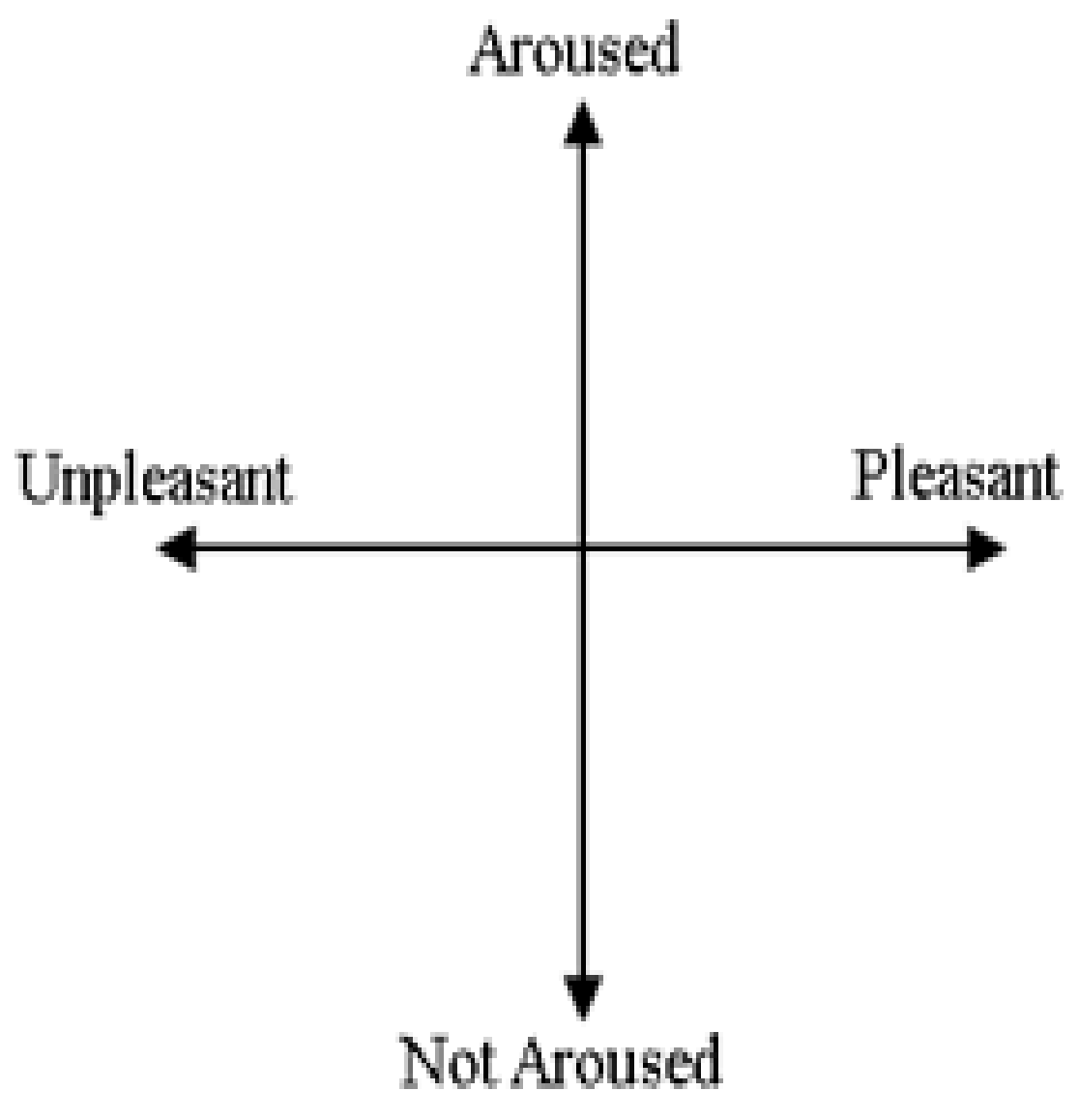
The remainder of the literature review is the basis for the study of the association between human emotion models and color. According to the emotion model of Russell, human emotion can be defined as an emotion model that is two-dimensional for the construction of various emotions such as the “Pleasant-Unpleasant” axis (X) and “Aroused-Not Aroused” axis (Y), as shown in
Figure 1 [
20]. Based on the emotion model of Russell, many studies have researched the relationship between color-based mapping for various emotional states and human emotion. Generally, visualized information can indicate the correlation between color and human emotion in the “Geneva Emotion Wheel [
24]”. In this case, human emotion is mapped into specific colors by dividing it into two dimensions: “Pleasant-Unpleasant” (X-axis) and “Arousal-Relaxation” (Y-axis), as indicated in
Figure 2.
We confirmed that these methods are used to analyze human emotions such as color components and the visual content of the surrounding environment [
20]. Based on these theories, we propose a method for analyzing the correlation between human emotion and temporal-spatial factors using a camera to capture the front environment and quantitatively extract visual context information from the acquired images. In the first step, the surrounding environment is photographed using the camera of a mobile device for image acquisition. Second, a subjective evaluation of the user is performed based on the acquired video for subsequent utilization as an index of the user’s emotional information. Third, a total of nine types of features are extracted from the acquired video: temporal complexity (#1), spatial complexity (horizontal edge (#2), vertical edge (#3)), color components (hue (#4), saturation (#5), intensity (#6), contrast (#7)), and sounds (amplitude (#8), frequency (#9)) to analyze the impact of each factor on human emotion. Finally, emotion estimation technology was developed by designing and analyzing a fully connected support vector regression (SVR) inference network based on the nine types of factors and the results of the subjective evaluation of the user.
3. Materials and Methods
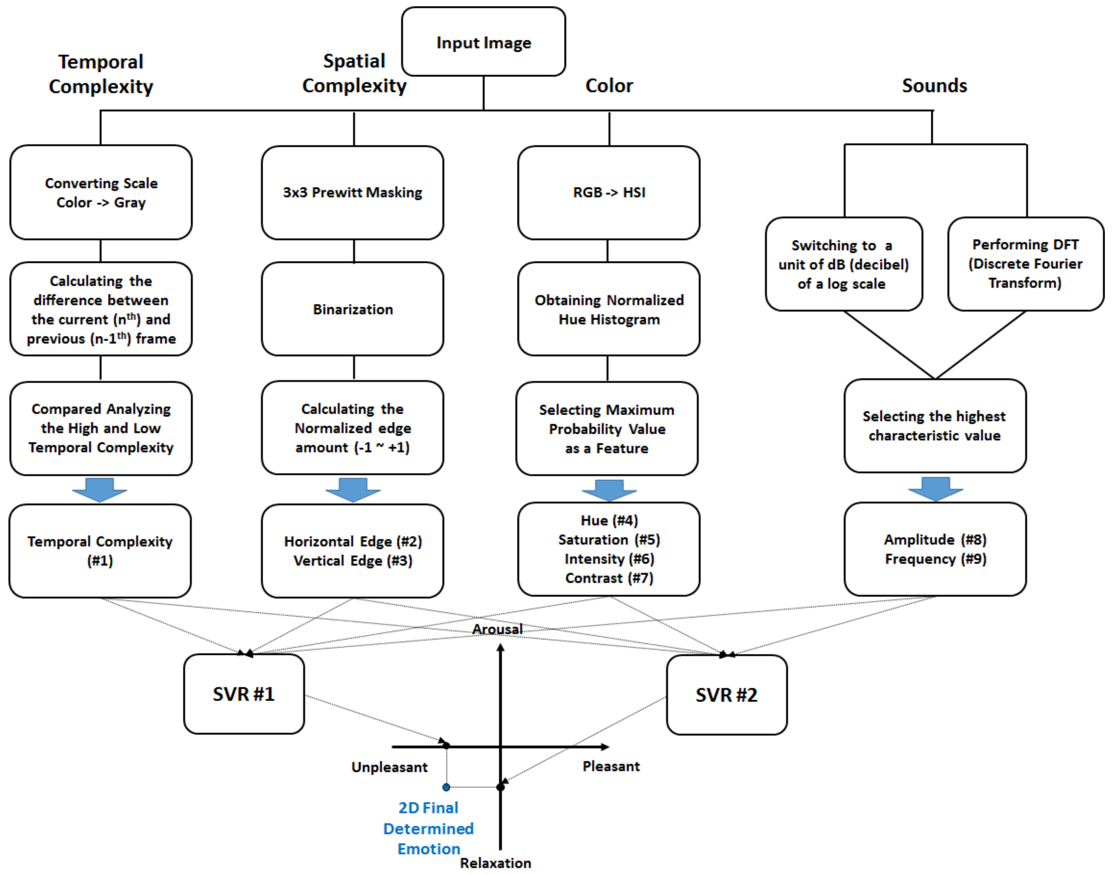
In this section, the temporal complexity, spatial complexity, color components, and sound detection methods are described using camera image processing. In this investigation, nine features were extracted from the input image, including temporal complexity (#1), horizontal edge (#2), vertical edge (#3), hue (#4), saturation (#5), intensity (#6), contrast (#7), amplitude (#8), and frequency (#9). An overall flowchart of the proposed method is shown in
Figure 3.
As above mentioned, nine features are provided as input data into two SVRs. Then, X-Y values are calculated through two SVRs. Finally, emotion position can be inferred as the two-dimensional model.
3.1. Used Features
3.1.1. Temporal Complexity
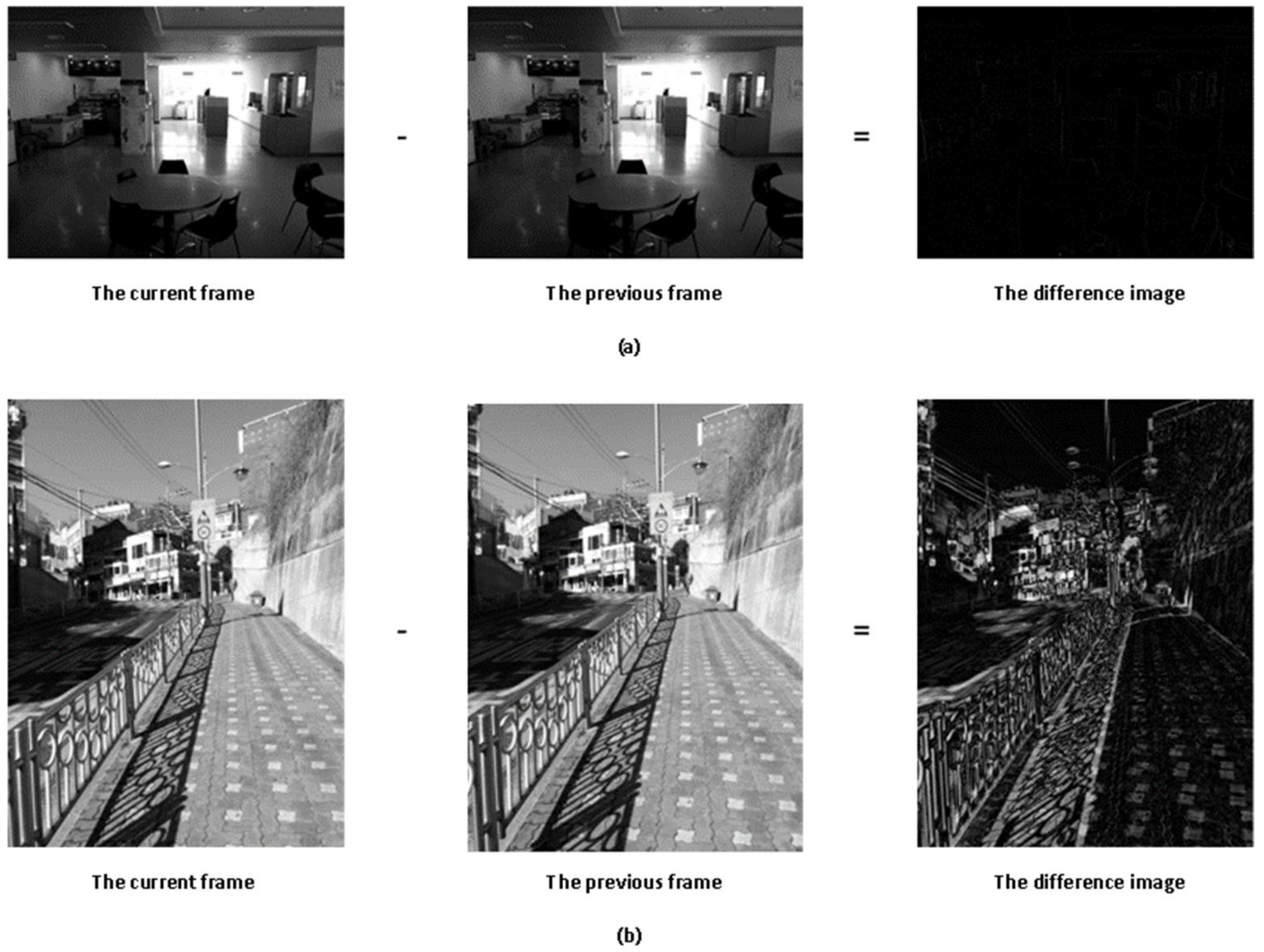
The temporal complexity (feature #1) represents the rate of change of motion by calculating the difference between the current frame image (nth) and the previous frame image (n-1st). In other words, the difference between pixels at the same position is calculated using the current frame and the previous frame and converting them into gray images. As an example, the temporal complexity of natural scenes was analyzed, as shown in
Figure 4. In the case of
Figure 4a, the temporal complexity is low in the current frame compared to the previous frame, according to the changing movement of the sky. In contrast, in the case of
Figure 4b, the temporal complexity can be seen as high in the current frame compared with the previous frame based on the rapidly changing movement of the roadside. The temporal complexity values ranged from 0 to 255. In this study, the calculated results for temporal complexity were used as values in the range from −1 to 1.
3.1.2. Spatial Complexity
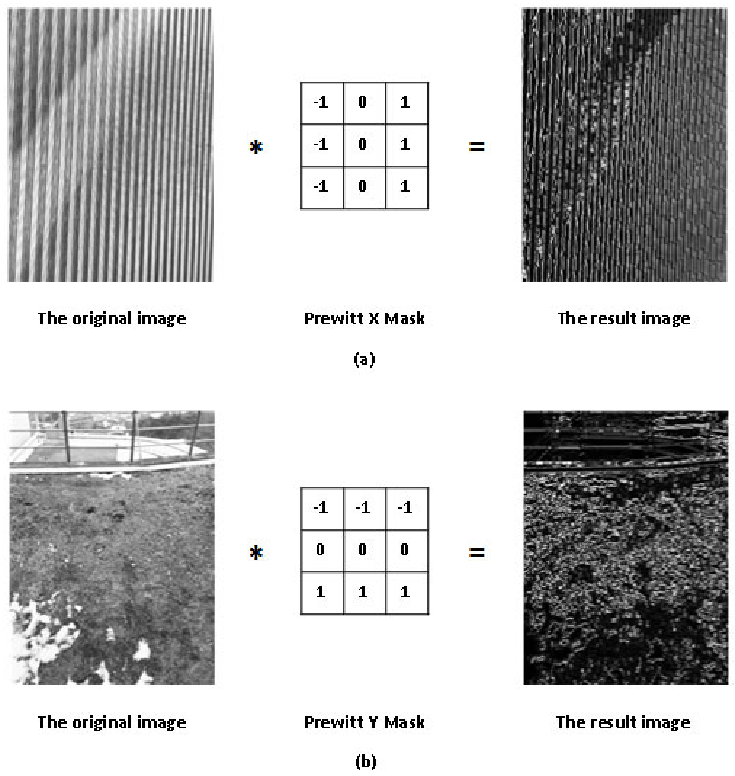
The spatial complexity is represented by detecting the boundary components by applying the Prewitt mask. In the detected boundary component image, the difference between the pixels at the same position is calculated using the mask. In this case, the spatial complexity is calculated as a horizontal edge (#2) and vertical edge (#3) using the Prewitt X and Y masks, respectively. In the case of
Figure 5a, the vertical components of spatial complexity can be acquired as large values based on the roadside using the Prewitt X mask. In contrast, the vertical edges are detected as large because of the lawn in
Figure 5b. The spatial complexity values range from 0 to 255. In this study, the calculated results of spatial complexity were used as values in the range of −1 to 1.
3.1.3. Color Components
In the color detection method, an image is analyzed to extract color components using a front-type camera as follows. Generally, color images are expressed in three channels: red (R), green (G), and blue (B). Because the components of the RGB color model imply both brightness and color, using this model for applications that use only color and brightness can be quite difficult. However, the limitations of the RGB model can be addressed using the HSI color model, which can separately represent images as hue (H), saturation (S), and intensity (I) values [
25]. Therefore, the first step of color conversion involves the conversion of RGB to HSI in the original image [
26]. In this case, each RGB channel is represented from 0 to 255. Therefore, it is more suitable to use the HSI model for color analysis. Finally, contrast (C) is obtained by calculating the standard deviation of the intensity.
Next, a normalized hue histogram is obtained on a scale of −1 to 1. In general, the hue component is distributed from 0° to 360° in the color space. In this case, the hue value of the color (
Valc) is calculated. In Equation (1), width and height are represented in the images as W and H, respectively. In addition, the number of hue values is denoted as “histo” in Equation (1). In this report, the parameter of the cosine function should be modified by adding 80° to compensate for the offset, because the angular offset is approximately 80° between the Geneva Emotion Wheel model and the hue of the HSI model. Consequently, the calculated results for the HSI were used as the values for the range of −1 to 1. In addition, a value in the range of −1 to 1 was used as the calculated result for contrast.
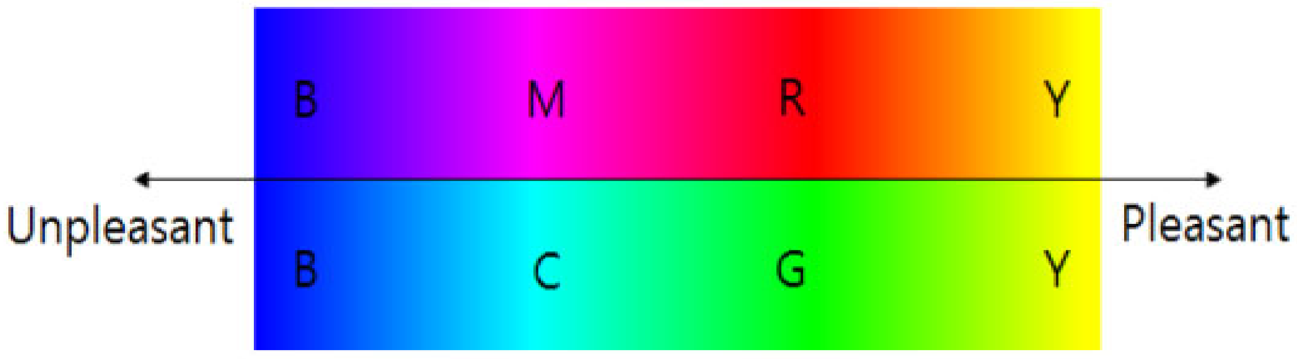
In this paper, six colors were estimated, including red (R), green (G), blue (B), cyan (C), magenta (M), and yellow (Y), based on the color psychology model. Then, the maximum frequency value was selected as a feature on the X-axis as “Pleasant-Unpleasant”. Consequently, six colors were mapped onto the X-axis of unpleasant to pleasant in the order of B, M, C, R, G, and Y, as shown in
Figure 6.
3.1.4. Sounds
Sound or voice is an element generated by a human being, such as talking, laughing, singing, crying, etc. Generally, the three major elements of sound are amplitude (size of the sound), pitch, and tone. Sounds can be expressed differently depending on their amplitude and size. For example, the amplitude or size of the pitch of a sound changes according to its frequency. The frequency can be determined from the sound height. Here, the frequency was analyzed using the discrete Fourier transform (DFT).
Amplitude is defined as a function representing the variation or distance of the sound when the periodic vibration exists. In general, the human ear is more sensitive to quiet sounds and less sensitive to loud sounds. Decibels (dB) that use a log scale are a generally used representation method of the sound amplitude. Here, by calculating an average value of the amplitude in acquired data for N seconds, then the size of the sound was used as a feature value. The amplitude was obtained in the range of −215 to 214.
Frequency is defined as a function that represents the cycle of the sounds which is how many times it repeats during a certain time period. A DFT is performed for obtaining the frequency by using the acquired data. Here, the DFT is computed for acquiring the specific frequency contents in waveform from multiple frequencies. Furthermore, the operation result shows how to constitute certain frequencies (Hz) in sounds. In this investigation, the sound frequency was determined by the acquired data for N seconds by using the DFT. Subsequently, the highest frequency values (Hz) in the results are used as the value of characteristics. In this case, the “dft()” function of the OpenCV library code was used to extract the frequency.
3.2. Analysis Methods
3.2.1. Acquiring Video of the Surroundings Using a Camera
To investigate how surrounding environmental factors can influence human emotions, the next step was performed. First, a video of the surrounding environment was acquired using a camera. In this case, the camera incorporated in a smartphone was used to acquire videos that were subsequently analyzed in real-time. To accomplish this task, we developed an Android application to capture videos of the surrounding environment. The developed Android application consisted of three parts. First, the specific scenarios of the experiments were described at the top of the screen. In brief, a large amount of video containing the desired scenes was acquired while walking around the campus. When an individual wished to capture a video while walking, this was performed by clicking the images in the middle of the screen, according to the experimental scenario. In this case, videos were recorded for 5 s.
3.2.2. Acquiring the Subjective Emotion Label for the Video
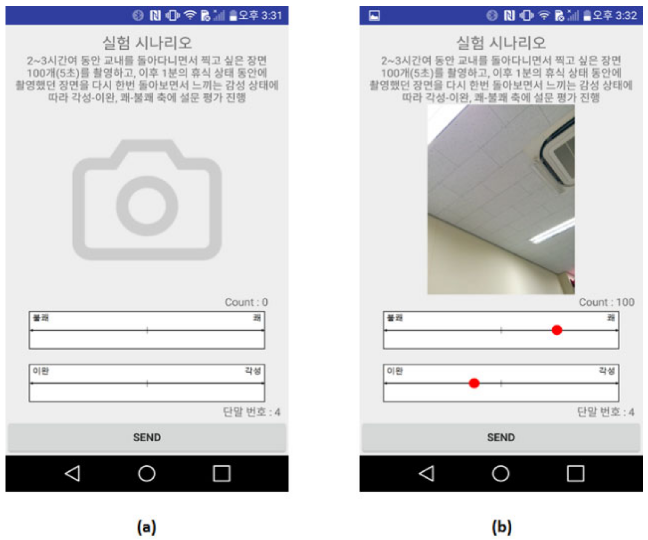
After capturing the videos, a subjective questionnaire evaluation was performed to evaluate the individuals’ emotional feelings from the captured videos related to the surrounding environments on the bottom of the screen, as shown in
Figure 7. More specifically, subjective evaluation was performed according to the emotional feeling using the bar graphs on the bottom of the screen in
Figure 7a,b. In
Figure 7a, the initial screen is described before performing the subject evaluation.
Figure 7b shows the screen until after subjective evaluation with the captured video is described. In this instance, the values range from −1.000 to 1.000 on the bar graphs. After both capturing videos of the surroundings using the smartphone camera and performing the subjective questionnaire evaluation, the value of the data was transferred to the server directly in real-time.
3.2.3. Extracting the Nine Features from the Videos
In this procedure, nine features were extracted from the videos, including temporal complexity (#1), spatial complexity (horizontal edge (#2), vertical edge (#3)), colors (hue (#4), saturation (#5), intensity (#6), contrast (#7)), and sounds (amplitude (#8), frequency (#9)). These characteristics are assumed to be quantitative factors that can affect human emotion as audiovisual factors and then nine features were defined. Each feature extraction method is described in
Section 3.1.
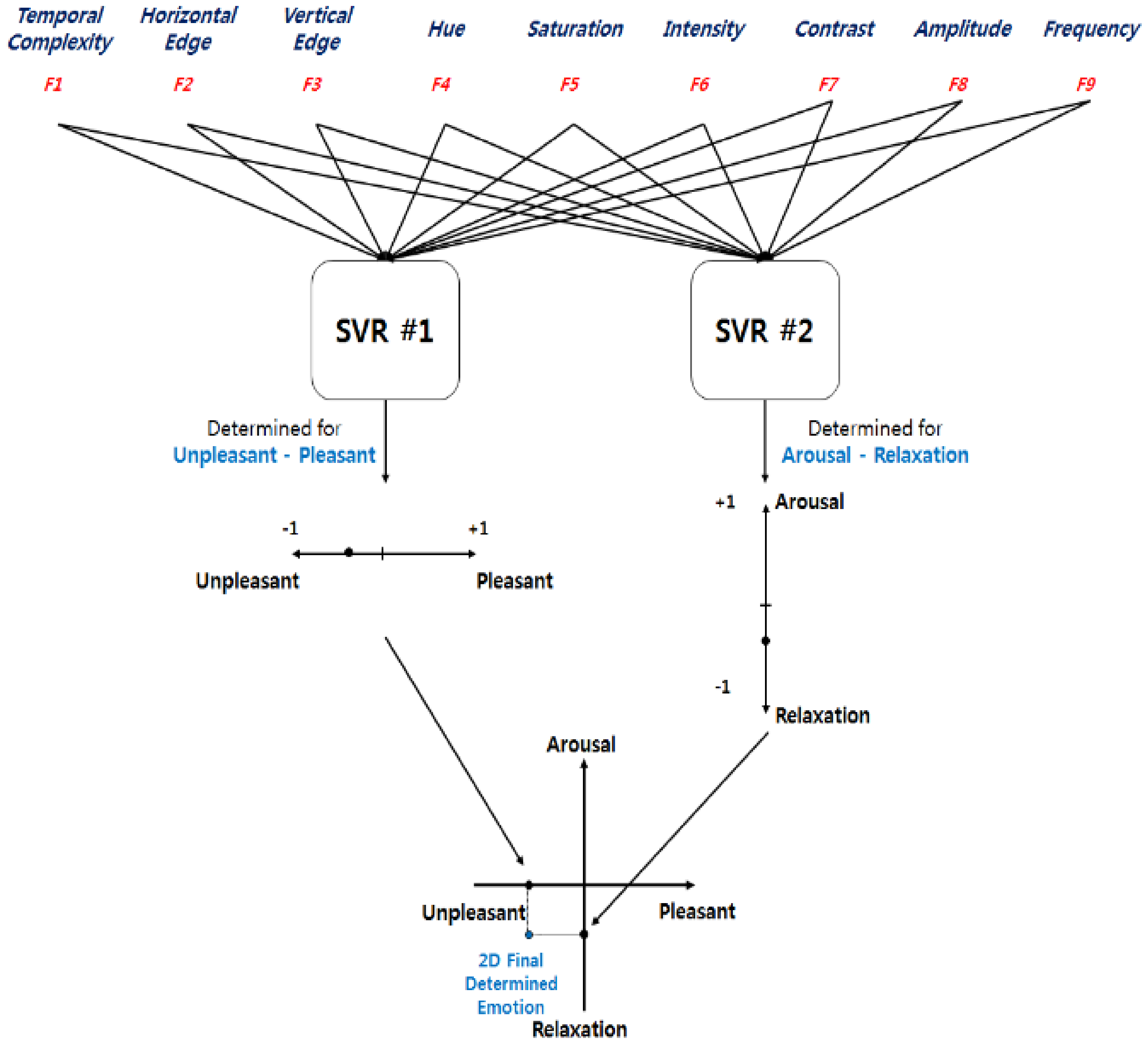
3.2.4. Emotion Estimation Using Support Vector Regression
In this study, support vector regression (SVR), which is a type of machine learning (a sub-concept of artificial intelligence (AI)), is adopted. Fully connected SVR networks were designed and applied to estimate emotional feelings based on the surrounding environment. Generally, to use SVR, two groups of data are needed for training and estimation. To estimate emotion, fully connected support vector regression (SVR) inference networks were designed to clarify the emotional decisions on the x-axis as “Unpleasant-Pleasant,” and those on the y-axis as “Arousal-Relaxation” in the two-dimensional model, as shown in
Figure 8. Specifically, nine features were used as input data according to SVR training from temporal complexity (#1) to frequency (#9).
Finally, the emotion parameters of the user are derived by analyzing the user’s surrounding environment based on the fully connected SVR inference. Using this approach, the current emotional state of the user can be inferred. Moreover, an interface that matches the emotions and situations of users is presented.
4. Experiments and Results
The experiments were performed twice for each subject group. In the first group, 30 subjects participated. In the second group, 66 subjects participated in the experiments. Thirty subjects participated voluntarily in the first experiment; these subjects consisted of postgraduate students in the Department of Computer Science, Emotion Engineering, and Mobile Software from Sangmyung University (male = 16, female = 14, mean age = ±27.1). The procedure of the experiment consisted of three parts as described in the experimental scenarios: taking videos and estimating the subjective evaluations, as shown in
Figure 9.
Firstly, the experimental scenarios were described for 3–5 min to 30 subjects before the start of the experiment. In addition, all 30 subjects were individually provided with smartphones. We also explained how to use the development application installed on the smartphone, as described in
Figure 9. Secondly, we instructed the subjects to take videos of the surrounding environment while walking around the university by clicking the camera images in the middle of the screen, as shown in
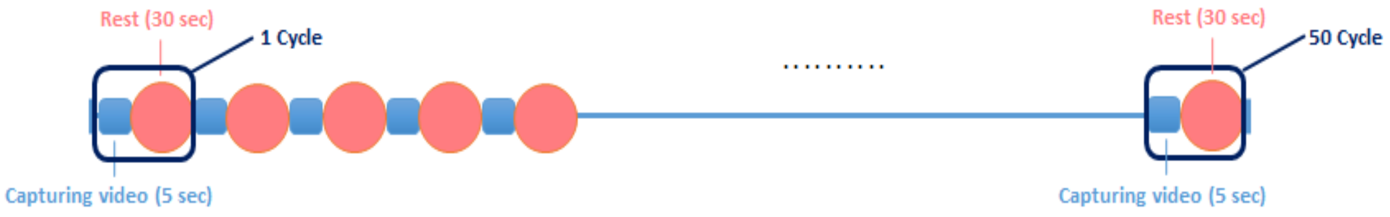
Figure 7a. In this case, the actual surrounding environment to capture via videos was recorded for 5 s in one shot. Lastly, subjective evaluation was performed according to emotional states on the axes of “Pleasant-Unpleasant” and “Arousal-Relaxation” while re-watching the scenes for 30 s using the bar graph on the bottom of the screen, as shown in
Figure 7a. In the subjective emotional evaluation, the values were estimated in a range from −1 to 1 on both the “Pleasant-Unpleasant” X-axis and the “Arousal-Relaxation” Y-axis. This process was performed 50 times by each subject.
For data collection, a total of 50 videos were acquired per subject. Consequently, a total of 1500 pairs of videos and subjective questionnaire evaluations were collected by 30 subjects (30 subjects × taking videos and subjective evaluations 50 times = collecting 1500 pairs). According to the previous section regarding the sequence of SVR-estimator execution, the 1500 collected datasets were separated into the training and test sets. In the experiment, 1000 of the 1500 data points were allocated to the training set, and the remaining 500 were allocated to the test set. In addition, fully connected dual SVR inference networks were used. The data type consisted of nine input data points extracted from videos and two output data points derived from SVR #1 and SVR #2. Specifically, the value of the x-axis as “Unpleasant-Pleasant” was determined using SVM #1. Similarly, the value of the y-axis as “Arousal-Relaxation” was determined using SVM #2.
In this report, the value of root mean square (RMS) error was calculated between the position of value used by the SVR estimator and the results for the subjective evaluation for measuring the accuracy of the proposed fully connected SVR network-based emotional evaluation owing to the surrounding environmental factors. The RMS error was calculated using the absolute value between x and y. For more details, X and Y were calculated by subtracting the absolute value of the square values of the validation and prediction according to the SVR estimator in “Pleasant-Unpleasant” and “Arousal-Relaxation”. Moreover, this software was implemented using C++ with OpenCV in real-time on a PC running Windows 10 OS, an Intel i5-6200U CPU at 2.4 GHz, 8 GB RAM, and a 23-inch display.
In addition, we constructed various cases according to the number of input four feature categories and analyzed the emotion estimation accuracy for each case. In this analysis, the nine features are categorized into four groups such as (1) Temporal complexity, (2) Spatial complexities (Horizontal and Vertical Edge), (3) Colors (Hue, Saturation, Intensity, Contrast), and (4) Sounds (Amplitude, Frequency). As a result, we could construct a total of 15 combinations as shown in
Table 1.
Finally, the comparison analysis was performed using all nine features for a total of 15 cases, as shown in
Table 2. Through the comparison analysis, we confirmed that the method of using all nine features is more effective in terms of the RMS error compared to three cases by using single, double, and triple features, respectively. In addition, we confirmed that using the multi-features method is more efficacious than the other methods for analyzing the impact of the combination of different factors in the surrounding environment on people.
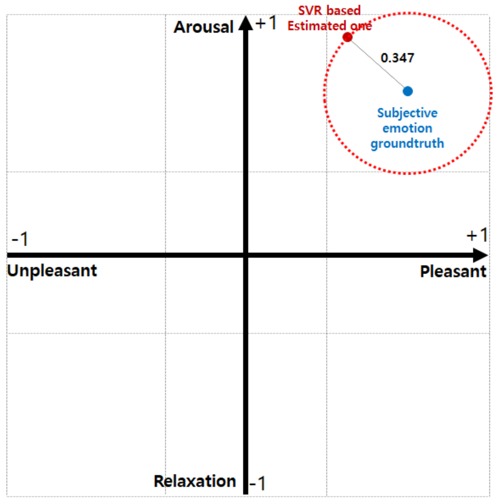
For the root mean square (RMS) error analysis of the dataset results, the error was represented as approximately 0.213 and 0.272 for the “Pleasant-Unpleasant” and “Arousal-Relaxation” categories, respectively. Furthermore, the average RMS error was 0.347 in the two-dimensional emotional plane. In other words, the distance of one diagonal line was approximately 0.35 when the two-dimensional region was divided into 3 × 3 grids, as shown in
Figure 10.
Consequently, the results between the subjectively evaluated emotion and the estimated emotion can be assumed to be in the same position in one column because the mean distance deduced from this study was estimated to be ±0.48. Based on this observation, we confirmed that the error results are within 12.5% of the result deduced by the SVR and the results of the actual human subjective evaluation of the 2D emotional plane.
5. Discussion
In this paper, experiments were conducted to recognize how the surrounding environment could affect human emotions, we confirmed several facts which will be highlighted. First, we performed RMS error analysis to analyze surrounding environments using SVR and confirmed which features are most discriminating among the nine features. Herein, we confirmed that the accuracy is higher and more reliable when using the multi features rather than when using a single feature. In that case, we confirmed that the results of error are within 12.5% between the result deduced by the SVR and the result of actual subjective evaluation on the 2D emotional plane when divided by a 3 × 3 grid and using the nine features. Based on these facts, we conclude that it is best to use nine features to judge human emotion through the surrounding environment videos.
However, the emotions experienced by people according to subjective evaluation are difficult to generalize because of individual variations in terms of the nine features associated with the surrounding environment. In other words, this work is limited in terms of attempting to generalize the results of human subjective emotions influenced by the surrounding environment. Therefore, in the future, it will be necessary to generalize the actual emotions that can be represented by many people due to the surrounding environment. In addition, this investigation deduces human emotions by using only the machine learning method. For further expansion, the research will be more useful to derive results that are more generalized than the methods presented in this paper through using artificial intelligence techniques such as deep learning.
6. Conclusions
In this paper, we proposed a method for analyzing the correlation between emotion and temporal-spatial factor information using a camera that can capture the frontal environment and quantitatively extract the visual context information from the acquired image. To this end, we developed a program that extracts temporal complexity, spatial complexity, specific color components, and sounds in real-time and can be analyzed by extracting nine features.
Experiments were conducted to recognize how the surrounding environment could affect human emotions; we confirmed the facts as follows. First, 1500 data were collected by the 30 participating subjects; we analyzed the surrounding environments with RMS error analysis by using the results of SVR, then confirmed which features were most discriminating among the nine features. Therefore, we confirmed that the accuracy is much higher and more reliable when using multiple features rather than when using a single feature. However, the emotion felt by people according to subjective evaluations cannot be effectively generalized because of individual variations in terms of the nine features among surrounding environment videos.
Consequently, the major limitations of this paper are that human emotion cannot be effectively generalized by individual variations as well as the lower recognition rate because of the feature-based method. Moreover, the results of human emotion inference were derived by using machine learning methods such as SVR not using deep learning. Therefore, in the future, it will be necessary to generalize the actual emotions that can be represented by many people through the surrounding environment. In addition, more research is needed to derive more general results than those presented in this paper using artificial intelligence techniques such as deep learning.
Author Contributions
Conceptualization, E.L.; methodology, E.L.; software, M.P.; validation, M.P.; formal analysis, M.P.; investigation, M.P.; resources, M.P.; data curation, M.P.; writing—original draft preparation, M.P.; writing—review and editing, E.L.; visualization, M.P.; supervision, E.L.; project administration, E.L.; funding acquisition, E.L. All authors have read and agreed to the published version of the manuscript.
Funding
This research was supported by a 2021 research grant from Sangmyung University.
Data Availability Statement
Not applicable.
Conflicts of Interest
The authors declare no conflict of interest.
References
- Cho, A.; Lee, H.; Jo, Y.; Whang, M. Embodied emotion recognition based on life-logging. Sensors 2019, 19, 5308. [Google Scholar] [CrossRef] [PubMed] [Green Version]
- Sellen, A.J.; Whittaker, S. Beyond Total Capture: A Constructive Critique of Lifelogging. Commun. ACM 2010, 53, 70–77. [Google Scholar] [CrossRef] [Green Version]
- Gurrin, C.; Smeaton, A.F.; Doherty, A.R. Lifelogging: Personal Big Data. Found. Trends Inf. Retr. 2014, 8, 1–125. [Google Scholar] [CrossRef]
- Park, Y.; Kang, B.; Choo, H. A Digital Diary Making System Based on User Life-Log. In Proceedings of the International Conference on Internet of Vehicles, Nadi, Fiji, 7–10 December 2016; pp. 206–213. [Google Scholar]
- Lin, R.X.; Yu, C.C.; Yang, H.L. A Deep Learning Approach to Extract Integrated Meaningful Keywords from Social Network Posts with Images, Texts and Hashtags. In ICT with Intelligent Applications, Proceedings of the ICTIS 2022, Ahmedabad, India, 22–23 April 2022; Springer: Cham, Switzerland, 2022; pp. 743–751. [Google Scholar] [CrossRef]
- Bayer, J.B.; Anderson, I.A.; Tokunaga, R. Building and breaking social media habits. Curr. Opin. Psychol. 2022, 45, 101303. [Google Scholar] [CrossRef] [PubMed]
- Al-Soliman, T.M. The Impact of the Surrounding Environment on People’s Perception of Major Urban Environmental Attributes. Archit. Plan. 1990, 2, 43–60. [Google Scholar]
- Bradley, M.M.; Hamby, S.; Löw, A.; Lang, P.J. Brain Potentials in Perception: Picture Complexity and Emotional Arousal. Psychophysiology 2007, 44, 364–373. [Google Scholar] [CrossRef]
- Bellizzi, J.A.; Hite, R.E. Environmental Color, Consumer Feelings, and Purchase Likelihood. Psychol. Mark. 1992, 9, 347–363. [Google Scholar] [CrossRef]
- How to Use Color Psychology to Give Your Business an Edge. Forbes/Entrepreneurs. 2014. Available online: http://www.forbes.com/sites/amymorin/2014/02/04/how-to-use-color-psychology-to-give-your-business-an-e-dge/ (accessed on 27 June 2022).
- Machajdik, J.; Hanbury, A. Affective Image Classification Using Features Inspired by Psychology and Art Theory. In Proceedings of the 18th ACM International Conference on Multimedia, Firenze, Italy, 25–29 October 2010; pp. 83–92. [Google Scholar]
- Schuller, B.; Hantke, S.; Weninger, F.; Han, W.; Zhang, Z.; Narayanan, S. Automatic Recognition of Emotion Evoked by General Sound Events. In Proceedings of the IEEE International Conference on Acoustics, Speech and Signal Processing (ICASSP), Kyoto, Japan, 25–30 March 2012; pp. 341–344. [Google Scholar]
- Yang, Y.H.; Chen, H.H. Machine Recognition of Music Emotion: A Review. ACM Trans. Intell. Syst. Technol. 2012, 3, 40. [Google Scholar] [CrossRef]
- Mehrabian, A.; Russell, J.A. The basic emotional impact of environments. Percept. Mot. Ski. 1974, 38, 283–301. [Google Scholar] [CrossRef] [PubMed]
- Li, Y.; Fei, T.; Huang, Y.; Li, J.; Li, X.; Zhang, F.; Khang, Y.; Wu, G. Emotional habitat: Mapping the global geographic distribution of human emotion with physical environmental factors using a species distribution model. Int. J. Geogr. Inf. Sci. 2021, 35, 227–249. [Google Scholar] [CrossRef]
- Van De Sande, K.E.; Gevers, T.; Snoek, C.G. Evaluating Color Descriptors for Object and Scene Recognition. IEEE Trans. Pattern Anal. Mach. Intell. 2010, 32, 1582–1596. [Google Scholar] [CrossRef] [PubMed]
- Zhou, B.; Lapedriza, A.; Xiao, J.; Torrabl, A.; Oliva, A. Learning Deep Features for Scene Recognition Using Places Database. Adv. Neural Inf. Process. Syst. 2014, 27, 487–495. [Google Scholar]
- Oliva, A.; Schyns, P.G. Diagnostic Colors Mediate Scene Recognition. Cogn. Psychol. 2000, 41, 176–210. [Google Scholar] [CrossRef] [PubMed] [Green Version]
- Peltonen, V.; Tuomi, J.; Klapuri, A.; Huipaniemi, J.; Sorsa, T. Computational Auditory Scene Recognition. In Proceedings of the International Conference on Acoustics, Speech and Signal Processing, Orlando, FL, USA, 13–17 May 2002; Volume 2, pp. II-1941–II-1944. [Google Scholar]
- Barrett, L.F.; Russell, J.A. The Structure of Current Affect Controversies and Emerging Consensus. Curr. Dir. Psychol. Sci. 1999, 8, 10–14. [Google Scholar] [CrossRef]
- Maglogiannis, I.; Vouyioukas, D.; Aggelopoulos, C. Face Detection and Recognition of Natural Human Emotion Using Markov Random Fields. Pers. Ubiquitous Comput. 2009, 13, 95–101. [Google Scholar] [CrossRef]
- Chen, L.S.; Huang, T.S.; Miyasato, T.; Nakatsu, R. Multimodal Human Emotion/Expression Recognition. In Proceedings of the Third IEEE International Conference on Automatic Face and Gesture Recognition, Nara, Japan, 14–16 April 1998; pp. 366–371. [Google Scholar]
- Gouizi, K.; Bereksi Reguig, F.; Maaoui, C. Emotion recognition from physiological signals. J. Med. Eng. Technol. 2011, 35, 300–307. [Google Scholar] [CrossRef] [PubMed]
- Sacharin, V.; Schlegel, K.; Scherer, K.R. Geneva Emotion Wheel Rating Study; NCCR Affective Sciences; Aalborg Universitet: Aalborg, Denmark, 2012. [Google Scholar]
- RGB to HSI. Available online: http://www.cse.usf.edu/~mshreve/rgb-to-hsi/ (accessed on 27 June 2022).
- Trivedi, V.K.; Shukla, P.K.; Pandey, A. Automatic segmentation of plant leaves disease using min-max hue histogram and k-mean clustering. Multimed. Tools Appl. 2022, 81, 20201–20228. [Google Scholar] [CrossRef]
- Hwang, H.; Ko, D.; Lee, E.C. Mobile App for Analyzing Environmental Visual Parameters with Life Logging Camera. In Advanced Multimedia Ubiquitous Engineering, Proceedings of the International Conference on Multimedia and Ubiquitous Engineering, Seoul, Korea, 22–24 May 2017; Springer: Singapore, 2017; pp. 37–42. [Google Scholar]
| Publisher’s Note: MDPI stays neutral with regard to jurisdictional claims in published maps and institutional affiliations. |
© 2022 by the authors. Licensee MDPI, Basel, Switzerland. This article is an open access article distributed under the terms and conditions of the Creative Commons Attribution (CC BY) license (https://creativecommons.org/licenses/by/4.0/).


