On the Use of the Multi-Agent Environment for Mobility Applications

Abstract

The multi-agent environment is now widely recognised as a key design abstraction for constructing multi-agent systems, equally important as the agents. An explicitly designed environment may have several roles, such as the inter-mediation between agents, the support for interaction, the embodiment of rules and constraints, etc. Mobility applications fit perfectly with a design in the form of a multi-agent system with an explicit environment model. Indeed, in these applications, the components of the system are autonomous and intelligent (drivers, travellers, vehicles, etc.), and the transportation network is a natural environment that they perceive and on which they act. However, the concept of the multi-agent environment may be profitably used beyond this specific geographical context. This paper discusses the relevance of the multi-agent environment in mobility applications and describes different use cases in simulation and optimisation.

1. Introduction

Large-scale and complex systems, in different socio-demographic contexts and various land-use configurations, could be analysed by modelling the behaviour and interactions of a large number of self-interested “agents”. The multi-agent paradigm provides a high level of detail and allows for the representation of non-linear phenomena and patterns that would be difficult to tackle with analytical approaches [1]. The multi-agent paradigm is a powerful model to design and implement transportation and mobility applications. Indeed, the multi-agent approach deals with systems consisting of many physically or logically distributed interacting components that possess some level of autonomy. These components can perceive their environment and react to changes following their goals. The authors in [2] listed several reasons for the preferred use of multi-agent systems in these applications, such as the natural and intuitive problem solving, the ability of autonomous agents to model heterogeneous systems, the ability to capture complex constraints linking all phases of problem-solving, etc. For Parunak [3], “agent-based modelling is most appropriate for domains characterised by a high degree of localisation and distribution”, which is the case for complex and dynamic transportation applications. The agent concept is well suited to represent travellers in transit or road traffic scenarios, for instance [4,5]. They are autonomous entities situated in an environment, adapt their behaviours to the dynamics they perceive, and interact with other agents to achieve specific goals.

There is a growing awareness in the multi-agent community that the multi-agent environment should be considered a primary design abstraction of equal importance to that of the agents. Models and architectures were proposed in the literature for the design of multi-agent environments, validated in a variety of application domains [6]. We believe that one of the domains of choice for modelling multi-agent environments is the transportation domain, especially the mobility applications. Indeed, transportation and mobility applications always have some representation of the environment, typically transportation networks of all modes. The environment in transportation applications has its own dynamics (e.g., traffic conditions, dynamic rules, weather, disruptions, etc.), which argues for its independent and explicit representation. Besides the intuitive representation of the transportation networks as the multi-agent environment, there are several other potential uses of the environment. In this paper, we illustrate different angles of multi-agent environment design in the context of transportation applications. The design of the environment can be considered at several levels of the system construction. It can represent a means of interaction between the agents. It can coordinate and synchronise the activities of the agents. It can also be designed as a mental model for agents to use in their reasoning and planning activities. In Figure 1, we provide three main layers for the design of the multi-agent environment in mobility applications. In the first layer (bottom figure), the environment is a spatial reference on which the agents act. It is also a reference for the resources available to agents, either for sensing or actuation purposes. The second layer (middle figure) is the spatio-temporal environment which extends the spatial environment with the time dimension for planning purposes. It also serves for historical data analysis, learning behaviours, and predicting future events. The third layer (top figure) is the communication environment is not related to the physical environment of the agents and is used for general-purpose communication between the agents. The first level corresponds to the traditional environment understanding and will not be detailed. In the remainder of this paper, we will describe the two other levels, we provide example models to specify them and examples of mobility applications to illustrate them. Note that the proposals for the three layers come from different communities and use cases and were never presented as part of the same model. Here, we try to unify these proposals in the same framework and describe them as different means to represent the multi-agent system’s environment.

The remainder of this paper is structured as follows. In Section 2, we present the environment as a spatio-temporal reference to the agents, usually for planing purposes, together with two example applications. In Section 3, we describe a generic design of multi-agent environment to support agents interaction. Section 4 concludes the paper and provides some future works.

2. Environment as a Spatio-Temporal Reference

The environment as a spatial reference is the most straightforward use of the multi-agent environment for mobility applications. A spatial environment provides a reference to the agents on which they can be located, on which they can move, and provides them with metrics to compute a distance between them. This use of the environment is the primary component provided by traffic simulation platforms such as SUMO [7], and general-purpose simulation platforms such as Repast Simphony [8]. The environment provides information about the present situation in the system, such as the positions of all the agents, the states of the entities (e.g., connected or non-connected vehicles), and the current constraints for the agents’ actions (e.g., traffic light signals states).

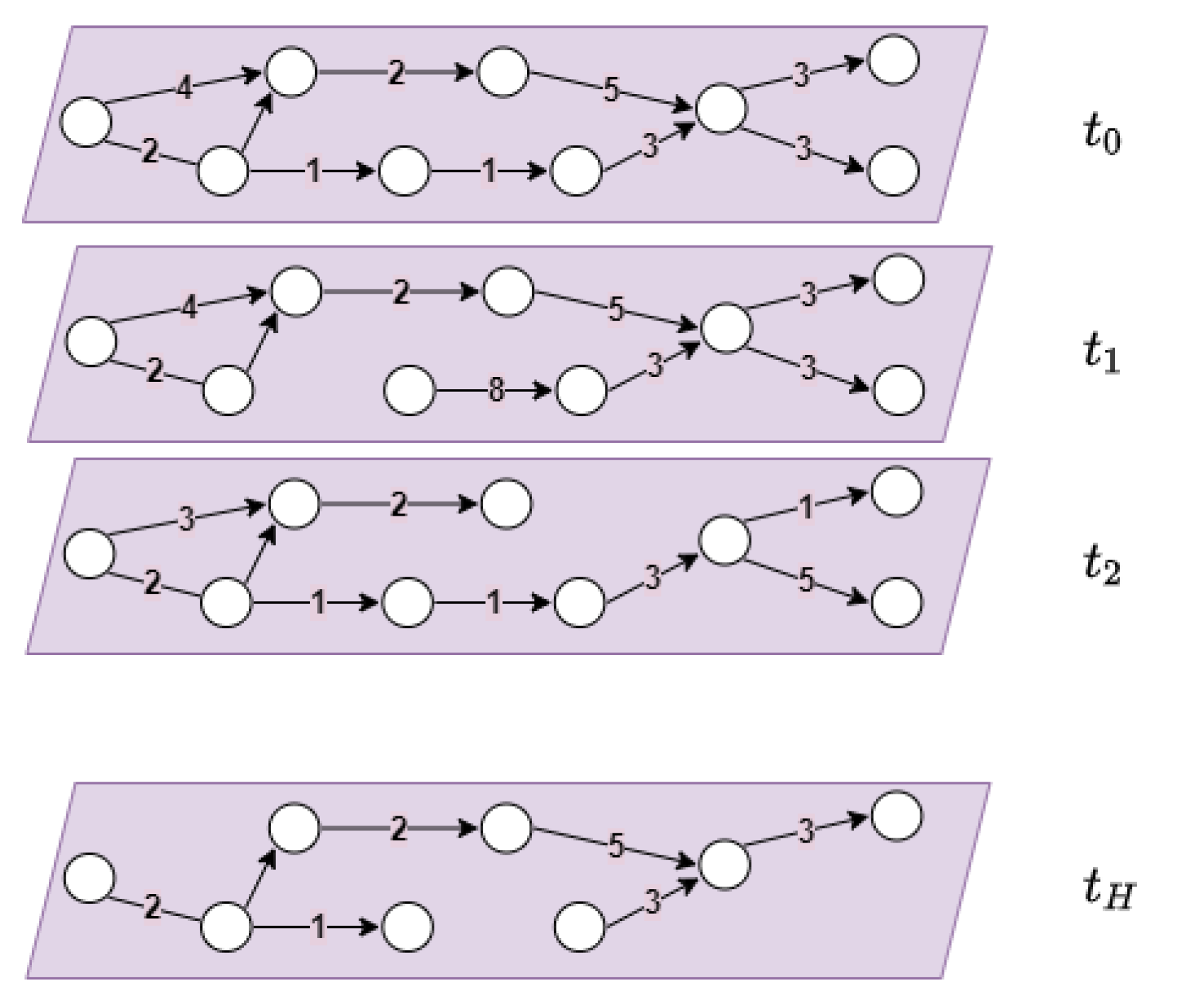
The environment as a spatial reference for the agents reflects the system’s present situation. Agents perceive the state of the environment before acting on it. However, cognitive agents usually have some planning activities and have a representation of the time, additionally to the space dimension. This section presents an approach where the multi-agent environment has two linked dimensions: space and time. This representation can either be used by the agents for planning, to reserve certain parts of the network at specific periods, for instance, or to synchronise agents’ actions and movements and also as a mental model for the agents, i.e., an internal knowledge representation of the dynamics of the networks through time.

2.1. Space–Time Model of the Environment

Let a transport network $G=(V,E)$, with a set of nodes $V=\left\{\left(v_i\right)\right\},i=0,...,N$ and a set of arcs $E=\left\{(v_i,v_j)\right|v_i\in V,v_j\in V,v_i\ne v_j\}$. Let two matrices $D=\left\{\left(d_{ij}\right)\right\}$ and $T=\left\{\left(t_{ij}\right)\right\}$ of costs, of dimensions $N\times N$ (the arc $(v_i,v_j)$ has a distance of $d_{ij}$ and a travel time of $t_{ij}$). The representation of the multi-agent environment is made of a duplication of G, H times, with H the maximum allowed time of the considered application: $G\left(t\right)=\left(N\right(t),E(t\left)\right)$, with $N\left(t\right)$ a set of nodes at time t and $E\left(t\right)$ a set of directed links at time t, and $0\le t\le H$. 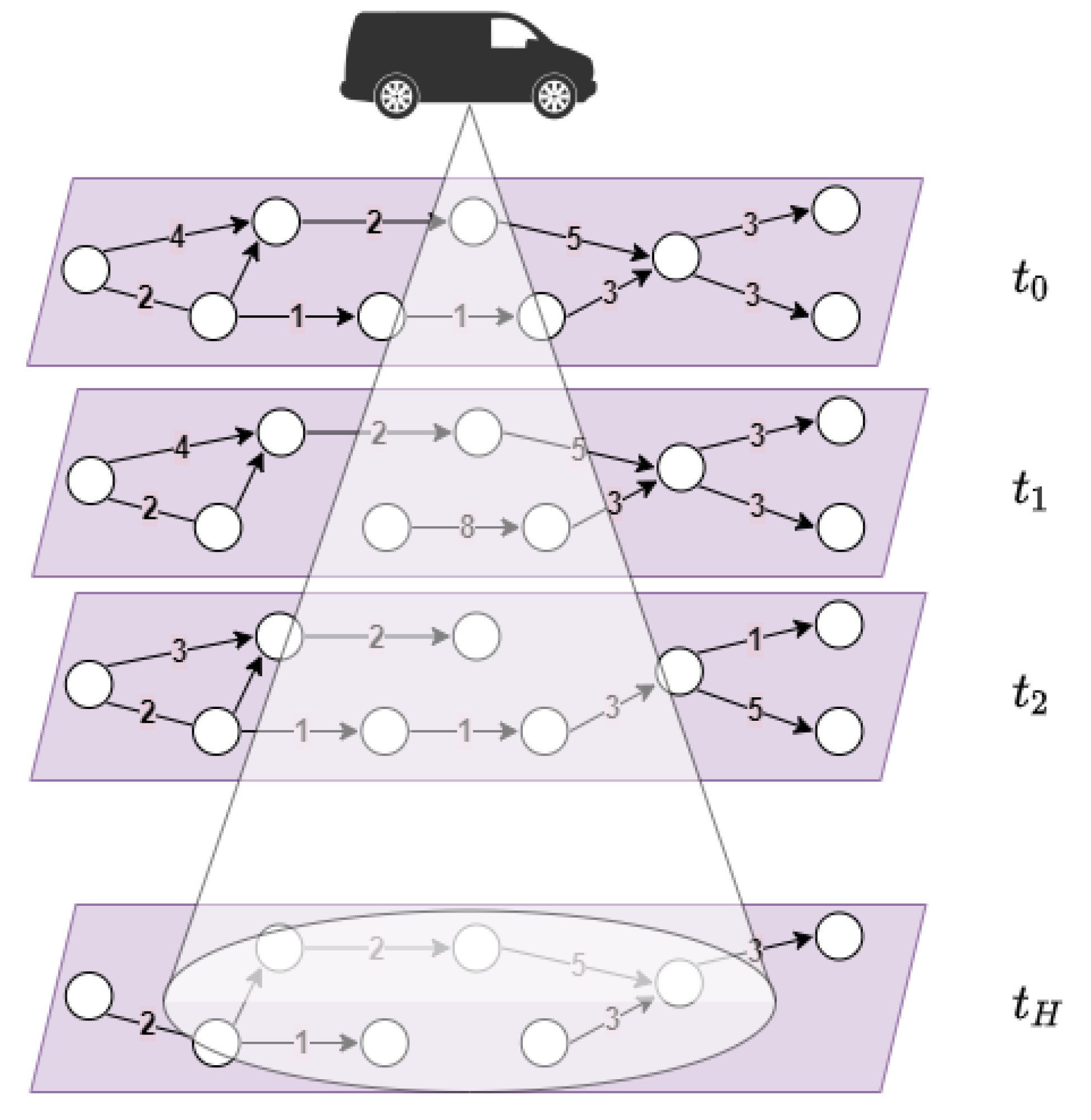The temporal copies of G are not necessarily identical (cf. Figure 2). Indeed, we can have different travel times between two copies of G to reflect the traffic state. Some nodes may be present in one copy while absent in another, to reflect the expansion of a crisis situation for instance [9]. Arcs may also be absent to reflect vehicle schedules in public transportation as in the application described in the next section. The costs on the edges usually refer to travel times.

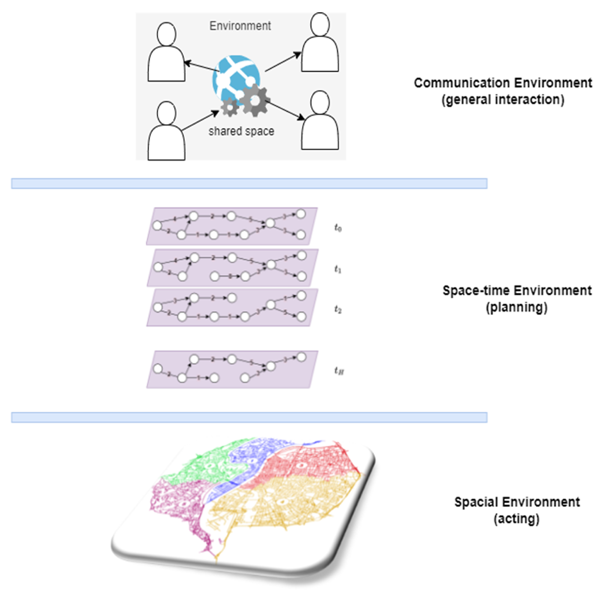
This representation of the multi-agent environment through time can be either a “passive” knowledge representation used by the agent to plan their future actions or to store historical states of the environment. It can also be used more profitably as an “active” entity, which is materialised as an explicit data structure, may have its dynamics, be accessed by all the agents and have a behaviour that can influence the behaviours of the agents.

So-called time-expanded graphs have long been used in the literature of transportation science, especially for transit networks, to compute shortest paths (e.g., [11,12]). The difference with the model presented in this paper is that the space–time network is active. It can act and react in the system and influence the behaviours of the agents. We describe this concept of active space–time environment with two mobility applications described in the following sections.

2.2. Space–Time Environment in Mobility Simulation

Transportation systems are becoming progressively complex as they are increasingly composed of intelligent and mobile entities. Travellers equipped with mobile devices and vehicles with connection capabilities allow passengers and vehicles to adapt their behaviour with up-to-date information. However, without control, the massive dissemination of information via billboards, radio announcements and individual guidance can have adverse effects and create new traffic concentrations and disruptions. Indeed, with this generalisation of real-time traveller information, the behaviour of modern transportation networks becomes more difficult to analyse and predict. It is then essential to properly observe these effects to consider the adequate methods to face them. To this end, we developed a multi-agent simulation platform that represents travellers, drivers, and public transportation vehicles and makes them move realistically on a multimodal transportation network. To allow travellers to receive only the disruption information relevant to them, the spatio-temporal network model described above is integrated into the simulation platform. In the following, we briefly introduce the multi-agent simulation platform, called SM4T (Simulator for Multi-agent MultiModal Mobility of Travelers) [13], before presenting our method of disseminating information to relevant travellers with spatio-temporal networks.

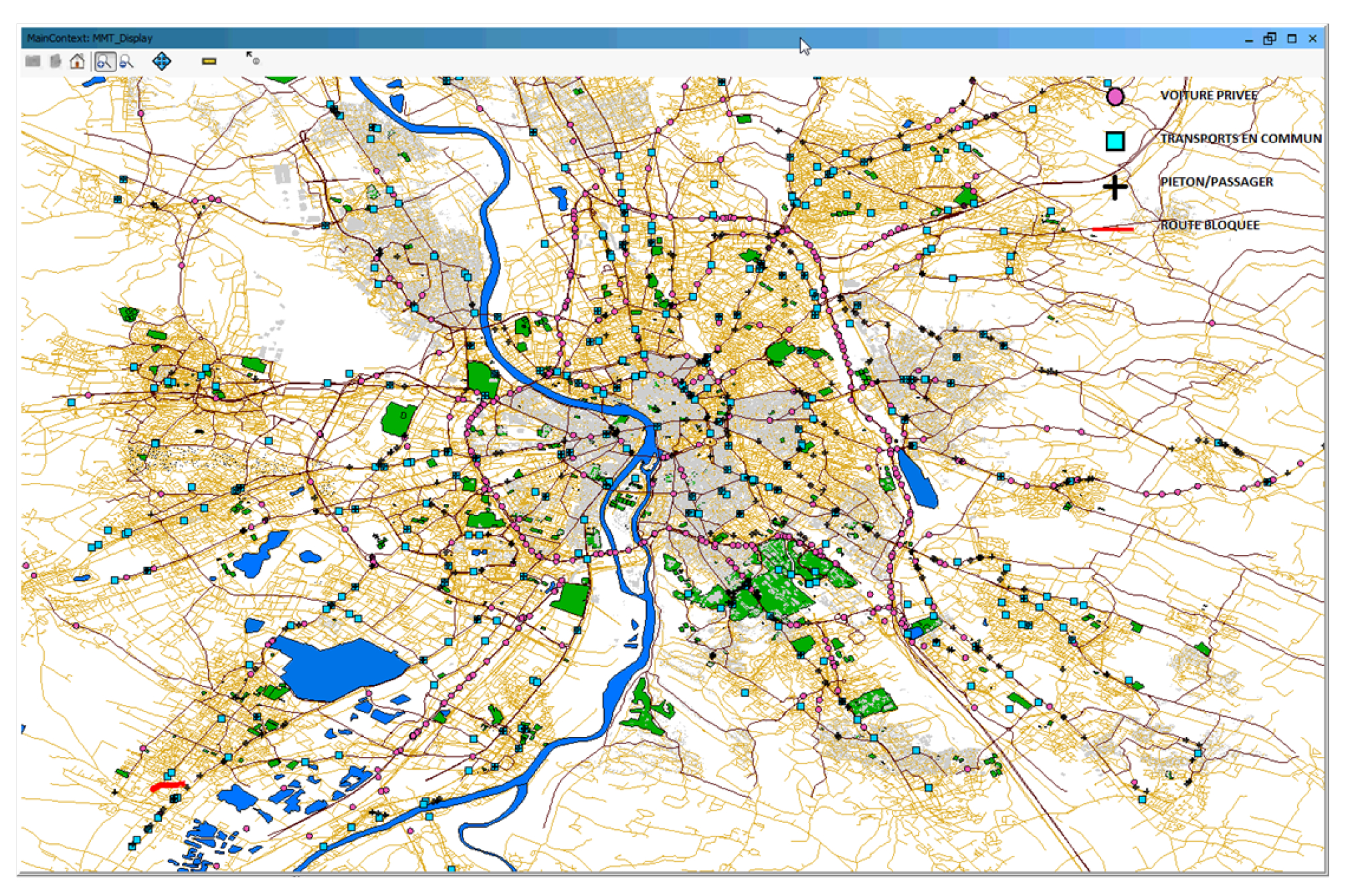
The multi-agent simulation platform that we designed and implemented allows for the individual representation of travellers moving on a transport network. We enrich it with traveller information capabilities, both at the stops and with personal information directly on the travellers’ smartphones. A simulation represents itinerary planners, passengers, public transportation vehicles, and information means in a micro-level and simulate their dynamic movements (cf. Figure 3).

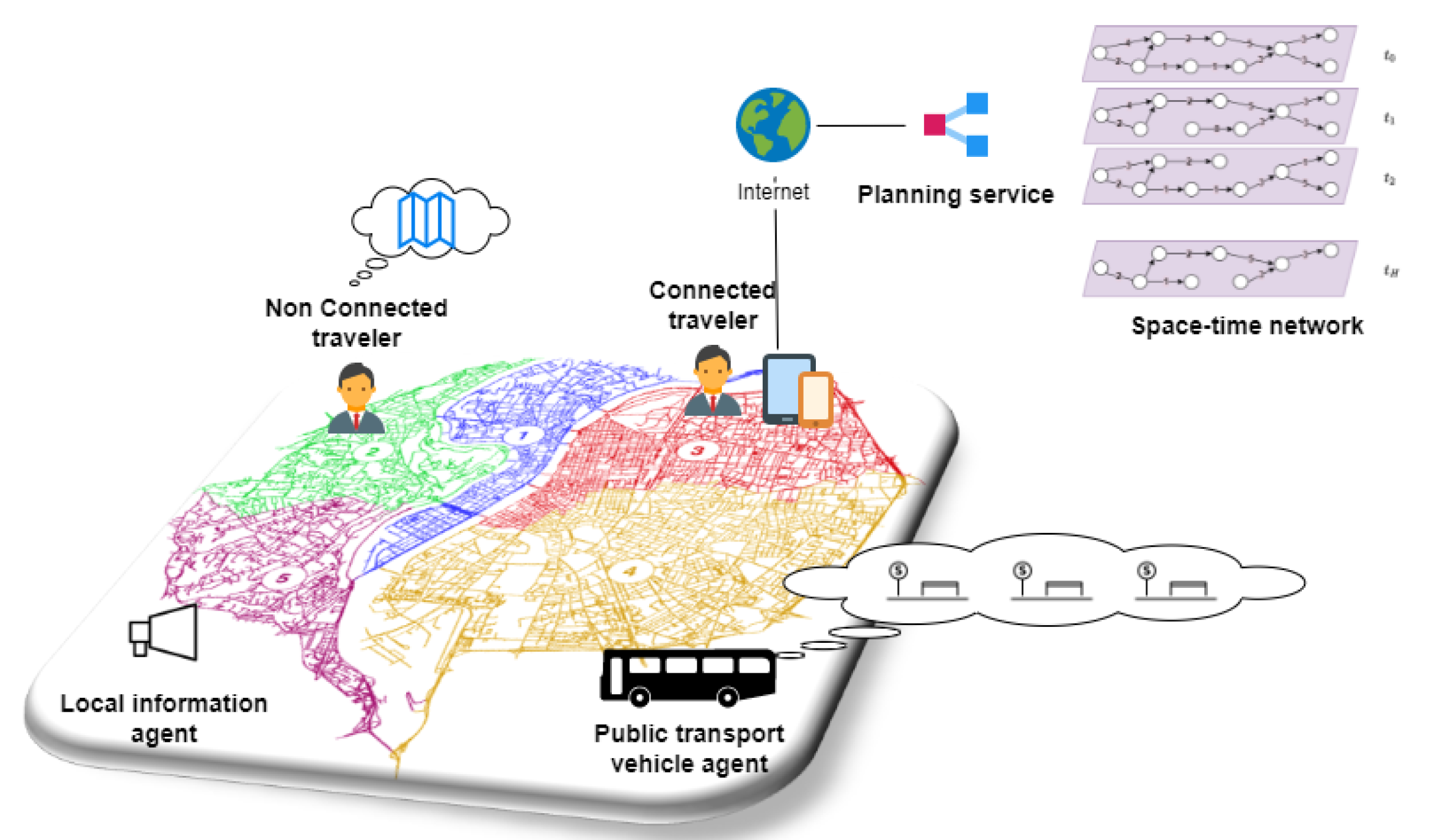
The multi-agent system of the simulator is composed of the following entities. We define four types of agents: Public transport vehicle agents (representing buses, metros, tramways, etc. in the system), Connected travellers, which represent the passengers that connect to real-time information sources, Non-connected travellers, that represent the travellers that only have a spatial representation of the network, and Local information agents, that provide real-time information locally on the stations of the network. A planning service is defined and is responsible for calculating the best route for the connected travellers only. It bases its calculation on the latest network status, including the ongoing disruptions (cf. Figure 4).

Non-connected travellers base their calculations on a static view of the network. They compute their shortest path based on this view. They wait for vehicles at scheduled stops and do not change their route until they either get stuck in an ongoing disruption (delay or line disconnection) or receive local information (from a Local information agent) about an ongoing disruption. When they receive the information, they infer the new network by applying the changes to their mental-and static-view of the transportation network and calculate a new shortest path based on this representation.

On the other hand, Connected travellers have their itineraries monitored by the Planning service. The latter uses the spatio-temporal network model defined earlier, representing the public transportation network, the network topology and the vehicle schedules. Recall that an arc connects two nodes $n_1\left(t\right)$ and $n_2\left(t\right)$ in $G\left(t\right)$ when there is a vehicle departing from $n_1$ to $n_2$ at t. Otherwise, the arc is absent. The spatiotemporal network is active in this application: the space–time arcs store listeners for traveller agents and inform them when the departure time or travel time changes or when the vehicle cancels its mission. To be aware of only the events that concern them, the Connected traveller agents subscribe to the only arcs of the multi-agent spatiotemporal environment that form their route. When the travel time of an arc or the departure time of the vehicle changes, the information is broadcast to the subscribed connected travellers. The planning process is then launched with the new network state.

Disruptions are modelled exclusively by modifying the space–time arcs (according to the vehicle schedules). Indeed, a vehicle’s delay is injected into the model by dynamically adjusting the space–time arcs representing the corresponding vehicle schedule, setting the destination node time to the delayed arrival times. Breakdowns are also modelled by removing the arcs corresponding to the vehicle’s mission from the space–time network. To model the failure of an entire line, the arcs representing the schedules of the remaining vehicles on the line are all deleted. As soon as a schedule is modified, based on the space–time network, the information is immediately detected by the relevant Connected agents, and only to them. Thus, when a timetable is modified, information about the delay or breakdown is sent only to connected travellers interested in these vehicles’ missions.

We executed the experiments with the data of the city of Toulouse in France. We chose this French city because we have detailed data about its network and a description of the travel patterns of the region [14]. The data came from Tisséo-SMTC, the public transportation authority of the Greater Toulouse. The public transportation network of Toulouse is composed of 80 lines, 359 itineraries and 3887 edges. Frequencies and edges costs are updated hourly. The multiagent system comprises 18,180 vehicles and from 5000 to 30,000 passengers. We define the number of ticks per simulation to 5000 for a journey from 6 am to 2 am. Every simulated tick corresponds to approximately 14 s. We chose the origins and destinations of passengers coherently with travel patterns of the region (the origins-destinations generation method is in [10]). We executed the simulations on a PC under Windows 7 with a processor Intel Xeon CPU E5-2630 (12 cores at 2 Ghz) with 50 GB of memory.

Previous works have shown that traveller information has little impact in case of minor disturbances. For this reason, we decided to use severe disorders instead in the form of complete disconnection of edges. In every simulation, we generated five random edge disconnections on the network during the whole simulation (one disconnection every 233 real-time minutes approximately). Every disconnection lasts 250 simulated ticks (slightly less than one hour in real-time). Due to edge disconnections, some passengers can no longer find an itinerary to their destination because edge disconnection impacts network connectivity. In the following results, these passengers were not considered (the ratio of passengers without an itinerary is stable, around 5% in all the simulations). Disturbances are random but concern only a certain number of edges that we consider significant to disconnect: the edges through which pass at least five different itineraries. We chose the five randomly disconnected edges between 21 candidate edges that satisfy this requirement.

We considered six different information level scenarios and executed each one 25 times. The first scenario is “the reference configuration” (to which we compared all the others) where no up-to-date information is provided to the passengers, neither local nor personalised. They only have the static description of the network and timetables. In the second scenario, the system provides only local information. The new travel times are available for the only passengers present at the considered stop. We did not consider any connected passengers in this scenario. The system provides local information at the stops in the remaining scenarios (3, 4, 5 and 6), and personal information is only available for the connected passengers. We considered 20%, 50%, 80%, then 100% of connected passengers, respectively, in these scenarios. In the scenarios with local information (all the simulations except the reference configuration), we placed local information agents in all the network stops. We report the average travel times for the passengers. We considered 30,000 passengers (approximately one-quarter of the actual number of passengers).

We executed this system twice: one time with a broadcast of the information about disturbances to all the connected passengers and once using the spatiotemporal network to circumscribe the sending to the only connected passengers. The impact of using the space–time environment on the number of exchanged messages is reported in

Table 1. Overall number of exchanged messages: broadcast versus space–time environment.

Ratio of Connected Travellers	Broadcast	Space–Time Network	Improvement
20%	634	252	60.25%
50%	1625	575	64.62%
80%	2680	944	64.78%
100%	3413	1105	67.62%

. It saves more than 60% of the messages in all the scenarios.

The use of the space–time multi-agent environment in this simulation platform makes the information exchange between agents more efficient and saves communication bandwidth. The impact of travellers’ real-time information is reported in [15].

2.3. Space–Time Environment for Planning in Mobility Applications

Vehicle routing problems (VRPs), modelling real-world applications such as dynamic carpooling or online food delivery, are complex optimisation applications that have attracted an enormous research effort for decades. In the online version of these problems, the optimisation of the response time to connected travellers is vital, along with the optimisation of the classical cost criteria (e.g., the size of the fleet of vehicles, the total travelled distance, the total travel times, the total waiting times, etc.). Multi-agent systems, on the one hand, and greedy insertion heuristics, on the other hand, are among the most promising approaches for this purpose. This section describes a multi-agent system coupled with a novel regret insertion heuristic. The heuristic is based on a space–time representation of the multi-agent environment. It serves as a mental model for the agents and as an explicit and active entity, guiding the planning of the agents.

In a VRP, many nodes must be visited once by several capacitated vehicles. These problems are challenging optimisation problems, and solving them has great practical utility. The time-constrained problem is one of the most studied variants of the VRP (Vehicle Routing Problem with Time Windows, VRPTW henceforth). In this variant, the vehicles must visit the nodes within time windows. Vehicle routing problems are divided into two categories: static problems and dynamic problems. In static problems, all the problem data is available before the optimisation process begins. In dynamic problems, the problem data is incomplete before the execution and is discovered progressively during the optimisation. The incomplete data can be any problem element, such as traffic data or available vehicles. However, the dynamic aspect usually refers to the travellers to be transported, which are unknown before execution (as in carpooling and dial a ride systems). Operational problems are never completely static, and it is reasonable to assume that a static system does not meet current operational configurations. Indeed, in real vehicle routing problems, even when all travellers are known in advance (with a reservation system, for example), there is always an element that makes the problem dynamic. These elements can be no-shows, delays, breakdowns, etc.

Online vehicle routing problems could be considered an extreme case of dynamic vehicle routing problems. Indeed, not only is the problem data not completely known before the optimisation starts, but travellers connect to the system in real-time and expect almost immediate responses to their requests. Therefore, the response time of the system in this type of problem is vital. It is more beneficial to immediately provide the current solution to the traveller, rather than waiting a long time for the optimisation system to improve its current solution slightly. Indeed, the traveller is unlikely to wait long for a response to her request.

To meet the requirement of short response times, we relied on the multi-agent paradigm to solve online vehicle routing problems. Multi-agent modelling of online VRPTW is relevant for the following reasons. On the one hand, since it allows the distribution of computations, it should shorten the response time to travellers’ requests. On the other hand, nowadays, vehicles are more and more connected and have onboard computing capabilities. In this context, the transportation system is de facto distributed and requires appropriate modelling to take advantage of these facilities. The multi-agent system (MAS) we describe in this section comprises vehicle agents, passenger agents, interface agents and planner agents. The multi-agent environment is explicitly modelled as a space–time network and used by the agents to plan their routes. The MAS simulates a distributed version of the so-called “insertion heuristic”. Insertion heuristics is a method of inserting individual travellers into vehicle routes. Each traveller is inserted into the route of the vehicle with the minimum marginal cost (the cost can refer to the detour incurred, for example). This method is the fastest known heuristic since there is no reconsideration of previous insertion decisions.

In heuristics and multi-agent methods in the literature, the hierarchical objective of minimizing the number of vehicles mobilised is considered to take priority over the overall costs (including the distance travelled by all vehicles). Most of the heuristics are based on a two-phase approach: minimizing the number of vehicles followed by minimizing the distance travelled [16]. The model we propose in this section aims at minimizing the number of vehicles used in priority while maintaining the use of a “pure” insertion heuristic, i.e., without any additional improvement to meet the response time requirements. To this end, our heuristic encourages vehicle agents to cover a maximum spatio-temporal area of the transportation network, avoiding the mobilisation of a new vehicle if a new traveller appears in an uncovered area.

A space–time pair $<i,t>$—with i a node and t a time—is said to be “covered” by a vehicle agent v if v can be in i at t. The “vehicle action zone” is the set of space–time nodes that the vehicle agent covers. In the context of online VRPTW, maximizing the action zones of the vehicle agents gives them a maximum chance to satisfy the demand of a future (unknown) traveller. By modelling the spatio-temporal action zones of the vehicle agents, we propose a new method to compute the price of inserting the traveller into a vehicle’s route. This proposal is a kind of regret insertion heuristic. Regret insertion heuristics, instead of choosing the vehicle with the minimum marginal cost, choose the vehicle and traveller with the greatest “regret”. Regret is a measure of the potential price to be paid if a given traveller were not immediately inserted into the route of a given vehicle. There are several methods for calculating regrets, such as the sum of the differences between all available prices and the minimum price [17].

2.3.1. Intuition of Spatio-Temporal Action Zones

Consider a vehicle agent v that has an empty route. Consider also a new traveller c described by: n a node, $[e,l]$ a time window, s a service time, and q a quantity. For v to fit c into its schedule, l must be large enough to allow v to be in n without violating its time constraints (if e is too small, v will have to wait until e). More precisely, the current time t plus the travel time from the depot to n must be less than or equal to l. Based on this observation, we define the action zone of a vehicle agent as the set of pairs $<n,t>$ of the space–time network that remains valid given its current route (n can be visited by the vehicle at t). The conical shadow in Figure 5 illustrates the action zone of a vehicle agent with an empty route.

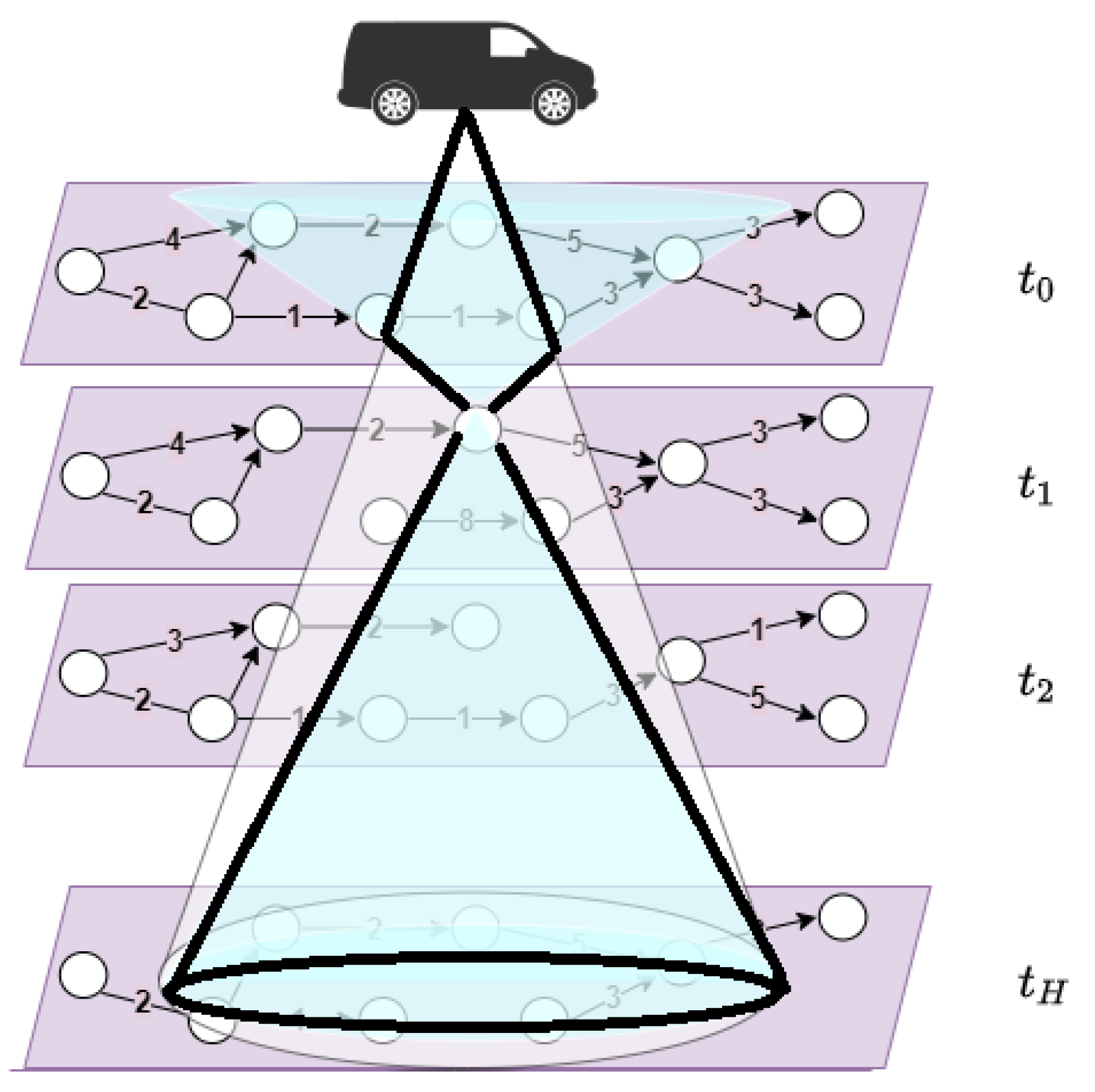
When a vehicle agent inserts a traveller into its route, it has to recalculate its action zone. Indeed, some pairs $<node,time>$ become unfeasible. In Figure 6, a new traveller is inserted into the vehicle route. The vehicle agent’s action zone after the traveller’s insertion is represented by the inside contour of the bold lines, which represent the space–time nodes that remain feasible after the insertion of the traveller.

The insertion price sent by a vehicle agent v to a traveller agent c corresponds to the hypothetical decrease in the action zone of v following the insertion of c in its route, i.e., the number of space–time nodes that would no longer be feasible. The idea is that the vehicle chosen for the insertion of a traveller is the one that keeps the maximum chance of being a candidate for the insertion of future travellers. Thus, the maximised criterion by the vehicle agents’ fleet is the sum of their action zones, i.e., the capacity of the MAS to react to the appearance of travellers without mobilizing new vehicles.

2.3.2. Coordination of Action Zones

Until now, the space–time model of the environment is used as a mental model of the agents, but it is not explicitly modelled and shared between the agents, and they do not interact with it. This method results in a better space–time coverage of the transportation network, materialised by a minimal mobilisation of vehicles with the appearance of new travellers. Each vehicle agent tries to maximise its action zone independently of the other agents with the mechanism mentioned above. However, it would be more interesting if the agents covered the network in coordination. Specifically, for a vehicle to lose space–time nodes that it alone covers should be more costly than losing nodes that the other agents cover.

To this end, we modelled the environment explicitly and associated with each node in the space–time network the list of vehicles that cover it. Each vehicle notifies the space–time nodes that it is part of its action zone, and each node continuously updates its list. Similarly, when a vehicle agent loses a node in its action zone, the node is notified, updating its list of vehicles.

When the price of inserting a traveller is calculated, each vehicle agent first determines the space–time nodes it would lose if it were to insert the new traveller. Then, it asks each of these nodes about the “price to be paid” if it were no longer covering it. This price is inversely proportional to the number of vehicles covering that node. Specifically, the price to pay is equal to

$$\frac{1}{|v_{<n,t>}|}$$

with $v_{<n,t>|}$ designating the vehicle agents covering the space–time node $<n,t>$ and $|v_{<n,t>}|$ the number of these vehicles.

This method, based on an active space–time environment, associates a higher penalty with the decision to stop covering a node less covered by others. Thus, vehicle agents have an incentive to cover the entire network in a coordinated manner.

Marius M. Solomon [18] created a set of different static problems for the VRPTW. It is now admitted that these problems are challenging and diverse enough to compare the different proposed methods with enough confidence. In Solomon’s benchmarks, six different sets of problems have been defined: C1, C2, R1, R2, RC1 and RC2. The travellers are geographically uniformly distributed in the problems of type R, clustered in the problems of type C, and a mix of uniformly distributed and clustered travellers is used in the problems of type RC. The problems of type 1 have narrow time windows (very few travellers can coexist in the same vehicle’s route) and the problems of type 2 have wide time windows. Finally, a constant service time is associated with each traveller, equal to 10 in the problems of type R and RC, and to 90 in the problems of type C. There are between 8 and 12 files containing 100 travellers in every problem set.

We chose to use Solomon benchmarks while following the modification proposed by [19] to make the problem dynamic. To this end, let $[0,T]$ the simulation time. All the time-related data (time windows, service times and travel times) are multiplied by $\frac{T}{l_0-e_0}$, with $[e_0,l_0]$ the scheduling horizon of the problem. The authors divide the travellers set into two subsets; the first subset defines the travellers known in advance, and the second is the travellers who reveal during execution. We did not make this distinction since we consider no travellers known in advance. An occurrence time is associated with each traveller, defining the moment when the system knows the traveller. Given a traveller i, the occurrence time that is associated is generated randomly between $[0,{\overline{e}}_i]$, with:

$$\begin{array}{c}\hfill {\overline{e}}_i=e_i\times \frac{T}{l_0-e_0}\end{array}$$

(1)

It is known that the behaviour of insertion heuristics is strongly sensitive to the appearance order of the travellers to the system. For this reason, we do not consider only one appearance order. We launch the process that we just described ten times with every problem file, creating ten different versions of every problem file.

We implemented two MAS with almost the same behaviour; the only difference concerns the measure used by vehicle agents to compute the insertion cost of a traveller. For the first implemented MAS, it relies on the Solomon measure (noted $\Delta$ Distance). The second relies on the space–time model (noted $\Delta$ Space–Time). We chose to run our experiments with the problems of class R and C, of type 1, which are the instances that are very constrained in time (narrow time windows).

For each problem class and type, we considered different travellers numbers to verify the behaviour of our model with respect to to the problem size. To this end, we considered the 25 first customers, the 50 first customers, and finally, all the 100 customers in each problem file.

Table 2. Results summary (criterion: fleet size).

	$\mathbf{\Delta }$ Distance	$\mathbf{\Delta }$ Space–Time
Problem	|Fleet|	|Fleet|
R1 25 customers	64	53
C1 25 customers	34	31
R1 50 customers	107	92
C1 50 customers	60	53
R1 100 customers	181	150
C1 100 customers	121	108

summarises the results. Each cell contains the best-obtained results with each problem class (the sum of all problem files). The results show, with the two classes of problems, that the use of the space–time model mobilises fewer vehicles than the traditional model ($53<64,31<34,92<107,53<60,150<181,108<121$). This result validates the intuition of the model, which consists of maximizing the future insertion possibilities for a vehicle agent.

The results show the superiority of this method, in terms of execution times and response times [20], and in terms of number of mobilised vehicles [21], compared to traditional methods.

3. Environment for Non-Spatial Interaction in Mobility Applications

The third layer in the environment models for multi-agent systems concerns the communication environment. The communication with traffic information or guidance, with a central server or with (non-local) acquaintances, belongs to this layer. This section presents an explicitly modelled multi-agent environment, which we show can have a relevant use in this context.

In dynamic transportation applications such as advanced traveller information systems or dial-a-ride systems, travellers, customers, and vehicles join the system nondeterministically and may also leave at any time. When specifying such open systems, the designer must define an architecture that allows for the integration of unknown agents. Newcomer agents must be able to find agents that have the properties, capabilities, or resources they need. To deal with this problem, known as the connection problem, the authors in [22] propose the concept of middle agents, which are the preferred interlocutors for agents seeking specific capabilities. The author in [23] presents recommendation systems, allowing the connection of distributed agents in open systems. This approach enables agents’ gradual and distributed construction of an address book. However, in dynamic transportation systems, the desired capabilities and information sources are usually known: transportation operators, vehicles, real-time traffic information providers, etc. The problem is knowing what information these sources generate is relevant to the new agents, whose context and needs are usually constantly changing. The multi-agent environment is also used for agent matching based on the properties of the agents and the exchanged objects or messages [24].

We adopted an environment-centric approach for agents’ interaction in mobility applications for these reasons: (i) it focuses on shared data; (ii) it allows selecting relevant information without having to know or maintain knowledge about the senders of this data. We propose a generic representation of the environment, shared by all agents in the system, allowing associative discovery of other agents and exchanging information between them. Agents do not maintain an address book of others and delegate the mapping of their preferences to the properties of others to the environment. They can also describe the properties of the agents they want to interact with and the messages they want to receive. The presence of a shared environment and the ability to define complex interaction constraints make this model an excellent candidate for the design of open and dynamic transportation systems.

This kind of shared spaces were initiated by Linda [25], which has known several extensions (e.g., Klaim [26], Mars [27] and Lime [28]). Linda-like models are based on the notion of a shared data repository. Agents communicate by exchanging tuples via an abstraction of an associative shared memory called the tuplespace. A tuplespace is a multiset of tuples (tuples duplication is allowed) and is accessed associatively (by contents) rather than by address. Every tuple is a sequence of one or more typed values. Communication in Linda is said to be generative: an agent generates a tuple and its life cycle is independent of the agent that created it. The model presented in this section is an extension of this model.

3.1. Model

Figure 7 illustrates the architecture of a multi-agent system following our generic model. The modelled MAS executes on a host, where (local) agents add, read and take objects to/from the environment. Every agent is either independent (like agents 1 and 2) or representing a non-modelled external system (traffic information server, for instance) or user (a traveller, for instance) in the MAS (like agents 3 and 4). The system agents interact with the environment via a shared space and don’t have to maintain an updated list of the agents and their properties and capacities.

For the specification of the system following this architecture, we adopt four primitives inspired by Linda [25] and a set of operators borrowed from Milner’s CCS [29]. A MAS adhering to the model is defined by a dynamic set of agents interacting with an environment-denoted ${\mathsf{\Omega }}_{ENV}$, which is composed of a dynamic set of objects. Agents can perceive (read-only) and/or receive (read and take) objects from the environment. Agents are defined by behaviour (a process), a state and local memory in which they store the data they perceive or receive from the environment. The primitives allowing these actions are the following [30]:

$$\mu ::=add\left(sds\right)\mid spawn(P,sds)\mid look(sd{s}_p,sd{s}_r,e)\mid update\left(sds\right)$$

The primitive $add\left(sds\right)$ adds to the environment an object described by $sds$. For instance, $add(position\leftarrow 1)$ adds the property-value pair $(position\leftarrow 1)$ to ${\mathsf{\Omega }}_{ENV}$. The primitive $spawn(P,sds)$ launches a new agent that behaves like P and which state is described by a description $sds$. For instance, $spawn(add(position\leftarrow 1),\{id\leftarrow a_1,position\leftarrow 1\})$ creates an agent that has $a_1$ as $id$ and 1 as $position$ and whose behaviour is $add(position\leftarrow 1)$. The primitive $look(sd{s}_p,sd{s}_r,e)$ allows object perception and reception (perception and removal from the environment). It blocks until a set of objects becomes present in ${\mathsf{\Omega }}_{ENV}$ such that the expression e is evaluated to $true$; the objects associated with the variables in $sd{s}_p$ are perceived and those associated with the variables in $sd{s}_r$ are received. For instance, the following instruction:

$$look\left(\right\{ticket\leftarrow t\},\{paper\leftarrow p\},t.destination=“Berlin”\wedge t.price\le budget$$

$$\wedge p.decision=“accepted”)$$

looks for two objects that will be associated with t and p. The object associated with t will be perceived, while the object associated with p will be received. After the execution of this instruction, the two objects will be present in the local memory of the caller agent. The latter will have two additional properties: $ticket$, which refers to the object associated with the variable t and $paper$, which refers to the object associated with p. The perceived $ticket$ has “Berlin” as destination and a $price$ lower than the budget of the executing agent, while the $received$ paper is “accepted” (the property $decision$ is equal to “accepted”).

The model thus proposes an environment-centric interaction for mobility applications. The advantages compared to point-to-point message exchanges or broadcasting messages to all agents are the following. On the one hand, in point-to-point message exchange, the agents (a traveller and a vehicle, for example) must be synchronised so that the transmission of a message by the first agent corresponds to its reception by the second. On the other hand, the sender must know the physical location of the receiver agent. With our approach, the communication is decoupled in time and space. Decoupling in time allows agents to communicate across time, i.e., their execution times do not have to overlap (the agents do not have to be synchronised by a rendezvous mechanism) to establish communication. The decoupling in space is related to the anonymous generation, and withdrawal of objects and messages from the shared space, i.e., agents do not have to know the location of other agents to communicate, so communication takes place independently of the location of the agents involved. Moreover, the shared space is an associative memory, i.e., data is accessed by content and not by address. In our model, the retrieval of data is not nominative but results from matching with a template, and the first data satisfying the template is returned in a non-deterministic manner.

Compared to the literature, our model provides improvements on two main aspects. On the one hand, we enrich the model with the property-values data structure instead of the tuple data structure. This enrichment results in a more powerful matching mechanism (replacing Linda-like templates). On the other hand, agents in our model have an observable state described by data. Indeed, state-of-the-art models describe what the agents do, not what they are. With agents’ states, agents can condition their interaction with their current context.

3.2. Example Application: Environment-Centred System for Traveller Information

In this section, we describe an application based on our model. We modelled and implemented a traveller information server. The purpose of the server is to inform online travellers about the status of the parts of the transportation network that concern them. Transportation Web services are represented with agents in the server, and their properties are related to the service or the information that they provide. The problem in this kind of application concerns the information flows that are dynamic and asynchronous. Indeed, each information source is hypothetically relevant. An agent cannot know a priori which information will interest him, since this depends on his context, which changes during execution [9].

The objective of this application is to ensure the information of a traveller about his ongoing trip (disturbances, alerts, alternative itinerary). This process is complex because the information sources are distributed, and the management of the follow-up assumes a comparison of all the available information. Using our environment model for this application allows designing an information server parameterised by its users (the travellers). We defined two categories of agents. The first concerns the agents representing the users (that we call PTA for Personal Travel Agent), while the second concerns the agents representing the transportation services (that we call Service Agent).

We implemented a multi-agent system running on a Web server for traveller information. Each Web service has a representation in the multi-agent environment, which is responsible for conveying messages from the server to the transportation Web service conversely. Every user is physically mobile and connects to the server via a transportation assistant app (TAA). During his connection, a PTA agent represents him inside the server, which is his interlocutor during his session. The context of the example is the following: inside the system, an agent represents a trip planning service, and an agent represents a traffic service responsible for the emission of messages related to incidents, traffic jams, etc. These agents are persistent since they are constantly associated with the service system. On the contrary, PTA agents representing the TAA in the system are volatile, created on a user’s connection and erased at the end of his session, i.e., when he/she arrives at destination.

Every stop of the network is described by a line number $line$ to which it belongs, and a number $number$ reflecting his position on the line. A user u is also described by his current position in the network (the properties $line$ and $number$). In a basic execution scenario, u has a path to follow during his trip, i.e. a sequence of tuples $\left\{\right(line,numbe{r}_{source},$$numbe{r}_{destination}{)}_i\mid i\in I\}$, with I the number of transportation means used by the traveller. Every tuple represents a part of the trip, without transfer. The TAA connects to the information server to receive his plan, and the agent u representing him is created. Then, the user is asked to specify his departure and his destination. Once this information is entered, u adds his planning demand in the environment. A demand is an object described by its properties: $emitter,subject$, etc. Afterwards, u keeps on listening to messages that are addressed to him, this way: $look(\varnothing ,\{message\leftarrow x\},x.receiver=id)$. The agent representing the trip planning service is listening to messages asking for a plan: $look(\varnothing ,\{request\leftarrow x\},x.subject=“plan”)$. As soon as he/she receives the message, he/she creates a message addressed to the trip planning Web service and awaits the response. When he/she receives the answer, a message is added to the environment addressed to u with the received plan as body: $add\left(\right\{emitter\leftarrow id,receiver\leftarrow request.emitter,body\leftarrow plan\left\}\right)$. The agent u, when he/she receives the message, analyses it and displays the result on the user’s TAA. Then, the agent u restrains his interaction to the messages concerning events coming up on his way. To do so, he/she executes the following action:

$$look(\varnothing ,\{event\leftarrow x\},\{x.subject=“alert”\},x.line=line\wedge x.number\ge number)$$

The agent u is interested in the alerts concerning his transportation plan, which are expressed by the preceding $look$ action. Let us assume that the agent representing the alert service adds an alert message concerning an accident on the way of u, resulting in a serious delay for him. The traveller, via his representing agent u, is notified concerning this alert event. Since the properties $line$ and $number$ are updated (with an $update$ action) at each move of u (each time he/she moves from stop to stop), the segment concerned by the alert messages gets gradually reduced until the end of the trip. The use of the environment, the constant update of the properties of the PTA agents, and the use of $look$ actions allowed us to maintain a continuous awareness of the traveller about problems occurring during his trip without relying on continuous requests to the server.

The proposal of an environment-centred system for traveller information shows how our model allows for the design and implementation of a dynamic and open transportation system. Agents join and leave the system freely and have complex interaction constraints. In this application, the interaction constraints concern the current positions and travellers’ itineraries.

4. Conclusions

This paper is based on the belief that multi-agent systems are an appropriate paradigm for modelling, simulating, and optimizing dynamic transportation applications [31]. It provides elements advocating that the explicit modelling of the multi-agent environment is a good choice for these applications. We proposed three layers of environment models that are interesting for designing transportation applications. The first layer concerns the spatial environment, which most approaches in the literature adopt. The second layer proposes a spatio-temporal model for interaction and is supported by a spatio-temporal representation of the environment. The third layer concerns shared spaces for general interaction between agents.

The design of the multi-agent environment as an explicit entity is often criticised for introducing centrality into systems that are supposed to be completely distributed. According to these arguments, centrality could lead to communication bottlenecks, low fault tolerance, and low scalability [32]. However, as we can see from the models and applications presented in this paper, this architecture has several advantages, and we believe there is a trade-off between the two visions. In our current work, we developed the idea that we can still benefit from an explicit representation of the multi-agent environment without losing the advantages of distribution, namely fault tolerance and scalability. To do so, we divided the design process into two phases. In the first phase, the system is designed with a conceptually centralised environment. In the second phase, the multi-agent environment is distributed [33]. We worked on environment distributions for each type of environment presented in this paper.

References

1. Bonabeau, E. Agent-based modelling: Methods and techniques for simulating human systems. Proc. Natl. Acad. Sci. USA 2002, 99, 7280–7287. [Google Scholar] [CrossRef] [PubMed] [Green Version]
2. Bazzan, A.L.; Klügl, F. A review on agent-based technology for traffic and transportation. Knowl. Eng. Rev. 2014, 29, 375–403. [Google Scholar] [CrossRef]
3. Parunak, H.V.D.; Savit, R.; Riolo, R.L. Agent-Based Modelling vs. Equation-Based Modelling: A Case Study and Users’ Guide. In Proceedings of Workshop on Modelling Agent Based Systems (MABS98), Paris, France, 4–6 July 1998. [Google Scholar]
4. Bessghaier, N.; Zargayouna, M.; Balbo, F. Management of urban parking: An agent-based approach. In Artificial Intelligence: Methodology, Systems, and Applications; Springer: Berlin/Heidelberg, Germany, 2012; pp. 276–285. [Google Scholar]
5. Bessghaier, N.; Zargayouna, M.; Balbo, F. An Agent-Based Community to Manage Urban Parking. Adv. Intell. Soft Comput. 2012, 155, 17–22. [Google Scholar]
6. Weyns, D.; Michel, F. (Eds.) Environments for Multi-Agent Systems IV, Fourth International Workshop; Lecture Notes in Computer Science; Springer: Berlin, Germany, 2015; Volume 9068. [Google Scholar]
7. Behrisch, M.; Bieker, L.; Erdmann, J.; Krajzewicz, D. SUMO-Simulation of Urban MObility—An Overview. In Proceedings of the Third International Conference on Advances in System Simulation, Barcelona, Spain, 23–29 October 2011; pp. 55–60. [Google Scholar]
8. Tatara, E.; Ozik, J. How to Build an Agent-Based Model III–Repast Simphony. In Proceedings of the Applied Agent-Based Modeling in Management Research, Academy of Management Annual Meeting, Chicago, IL, USA, 7–11 August 2009. [Google Scholar]
9. Zargayouna, M. Une repréSentation Spatio-Temporelle de l’Environnement pour le Transport À la Demande. Workshop Represent. Reason. Time Space 2005. Available online: https://basepub.dauphine.psl.eu/bitstream/handle/123456789/5925/plugin-publi288.pdf?sequence=2 (accessed on 9 February 2022).
10. Ksontini, F.; Zargayouna, M.; Scemama, G.; Leroy, B. Building a realistic data environment for multiagent mobility simulation. In Proceedings of the KES International Symposium on Agent and Multi-Agent Systems: Technologies and Applications, Tenerife, Spain, 15–17 June 2016; Springer: Cham, Switzerland, 2016; Volume 58, pp. 57–67. [Google Scholar]
11. Pyrga, E.; Schulz, F.; Wagner, D.; Zaroliagis, C. Efficient models for timetable information in public transportation systems. J. Exp. Algorithmics 2008, 12, 1–39. [Google Scholar] [CrossRef]
12. Schulz, F.; Wagner, D.; Zaroliagis, C. Using multi-level graphs for timetable information in railway systems. In Workshop on Algorithm Engineering and Experimentation; Springer: Berlin, Germany, 2002; pp. 43–59. [Google Scholar]
13. Zargayouna, M.; Othman, A.; Scemama, G.; Zeddini, B. Impact of travellers information level on disturbed transit networks: A multiagent simulation. In Proceedings of the 2015 IEEE 18th International Conference on Intelligent Transportation Systems, Gran Canaria, Spain, 15–18 September 2015; pp. 2889–2894. [Google Scholar]
14. Zargayouna, M.; Zeddini, B.; Scemama, G.; Othman, A. Simulating the impact of future internet on multimodal mobility. In Proceedings of the 2014 IEEE/ACS 11th International Conference on Computer Systems and Applications (AICCSA), Doha, Qatar, 10–13 November 2014; pp. 230–237. [Google Scholar]
15. Zargayouna, M. Multiagent simulation of real-time passenger information on transit networks. IEEE Intell. Transp. Syst. Mag. 2020, 12, 50–63. [Google Scholar] [CrossRef]
16. Nagata, Y.; Bräysy, O.; Dullaert, W. A penalty-based edge assembly memetic algorithm for the vehicle routing problem with time windows. Comput. Oper. Res. 2010, 37, 724–737. [Google Scholar] [CrossRef]
17. Friggstad, Z.; Swamy, C. Approximation algorithms for regret-bounded vehicle routing and applications to distance-constrained vehicle routing. In Proceedings of the Forty-Sixth Annual ACM Symposium on Theory of Computing, New York, NY, USA, 31 May–3 June 2014; pp. 744–753. [Google Scholar]
18. Solomon, M. Algorithms for the vehicle routing and scheduling with time window constraints. Oper. Res. 1987, 15, 254–265. [Google Scholar] [CrossRef] [Green Version]
19. Gendreau, M.; Guertin, F.; Potvin, J.Y.; Taillard, E.D. Parallel tabu search for real-time vehicle routing and dispatching. Transp. Sci. 1999, 33, 381–390. [Google Scholar] [CrossRef] [Green Version]
20. Zargayouna, M.; Zeddini, B. Dispatching Requests for Agent-Based Online Vehicle Routing Problems with Time Windows. J. Comput. Inf. Technol. 2020, 28, 59–72. [Google Scholar] [CrossRef]
21. Zargayouna, M.; Zeddini, B. Fleet organization models for online vehicle routing problems. In Transactions on Computational Collective Intelligence VII; Springer: Berlin/Heidelberg, Germany, 2012; pp. 82–102. [Google Scholar]
22. Sycara, K.; Wong, H. A Taxonomy of Middle-Agents for the Internet. In Proceedings of the Fourth International Conference on MultiAgent Systems (ICMAS-2000), Washington, DC, USA, 10–12 July 2000; pp. 465–466. [Google Scholar]
23. Vercouter, L. Conception et Mise en Oeuvre de Systèmes Multi-Agents Ouverts et Distribués. Ph.D. Thesis, Ecole Nationale Supérieure des Mines de Saint-Etienne, Université Jean Monnet-Saint-Etienne, Saint-Étienne, France, 2000. [Google Scholar]
24. Zargayouna, M.; Trassy, J.S.; Balbo, F. Property Based Coordination. In Artificial Intelligence: Methodology, Systems, Applications; Springer: Berlin/Heidelberg, Germany, 2006; Volume 4183, pp. 3–12. [Google Scholar]
25. Gelernter, D. Generative communication in linda. ACM Trans. Program. Lang. Syst. 1985, 7, 80–112. [Google Scholar] [CrossRef]
26. Nicola, R.; Ferrari, G.L.; Pugliese, R. Klaim: A Kernel Language for Agents Interaction and Mobility. IEEE Trans. Softw. Eng. 1998, 24, 315–330. [Google Scholar] [CrossRef] [Green Version]
27. Cabri, G.; Leonardi, L.; Zambonelli, F. Reactive tuple spaces for mobile agent coordination. In MA’98: Proceedings of the Second International Workshop on Mobile Agents; Springer: Berlin, Germany, London, UK, 1999; pp. 237–248. [Google Scholar]
28. Picco, G.P.; Murphy, A.L.; Roman, G.-C. LIME: Linda meets mobility. In Proceedings of the International Conference on Software Engineering, Los Angeles, CA, USA, 16–22 May 1999; pp. 368–377. [Google Scholar]
29. Milner, R. Communication and Concurrency; Prentice-Hall: Hoboken, NJ, USA, 1989. [Google Scholar]
30. Zargayouna, M.; Balbo, F.; Scemama, G. A data-oriented coordination language for distributed transportation applications. In KES International Symposium on Agent and Multi-Agent Systems: Technologies and Applications; Springer: Berlin/Heidelberg, Germany, 2009; pp. 283–292. [Google Scholar]
31. Zargayouna, M. Multiagent Environments for Dynamic Transportation Applications. In KES International Symposium on Agent and Multi-Agent Systems: Technologies and Applications; Springer: Berlin/Heidelberg, Germany, 2017; pp. 12–21. [Google Scholar]
32. Billhardt, H.; Fernández, A.; Lujak, M.; Ossowski, S.; Julián, V.; De Paz, J.F.; Hernández, J.Z. Towards Smart Open Dynamic Fleets. In Multi-Agent Systems and Agreement Technologies: 13th European Conference, EUMAS 2015, and Third International Conference, AT 2015, Athens, Greece, 17–18 December 2015; Rovatsos, M., Vouros, G., Julian, V., Eds.; Springer International Publishing: Cham, Switzerland, 2016; pp. 410–424. [Google Scholar] [CrossRef]
33. Mastio, M.; Zargayouna, M.; Scemama, G.; Rana, O. Distributed agent-based traffic simulations. IEEE Intell. Transp. Syst. Mag. 2018, 10, 145–156. [Google Scholar] [CrossRef]
Figure 1. Layers of multi-agent environment.
Futureinternet 14 00132 g001
Figure 2. Space–time network.
Futureinternet 14 00132 g002
Figure 3. Interface of SM4T.
Futureinternet 14 00132 g003
Figure 4. Architecture of the multi-agent system.
Futureinternet 14 00132 g004
Figure 5. Initial spatio-temporal action zone.
Futureinternet 14 00132 g005
Figure 6. Action zone after insertion of a traveller.
Futureinternet 14 00132 g006
Figure 7. Architecture of a Multi-agent system with general-purpose explicit environment.
Futureinternet 14 00132 g007