A Machine Learning Predictive Model to Detect Water Quality and Pollution

Abstract

The increasing prevalence of marine pollution during the past few decades motivated recent research to help ease the situation. Typical water quality assessment requires continuous monitoring of water and sediments at remote locations with labour-intensive laboratory tests to determine the degree of pollution. We propose an automated water quality assessment framework where we formalise a predictive model using machine learning to infer the water quality and level of pollution using collected water and sediments samples. Firstly, due to the sparsity of sample collection locations, the amount of sediment samples of water is limited, and the dataset is incomplete. Therefore, after an extensive investigation on various data imputation methods’ performance in water and sediment datasets with different missing data rates, we chose the best imputation method to process the missing data. Afterwards, the water sediment sample will be tagged as one of four levels of pollution based on some guidelines and then the machine learning model will use a specific technique named classification to find the relationship between the data and the final result. After that, the result of prediction can be compared to the real result so that it can be checked whether the model is good and whether the prediction is accurate. Finally, the research gave improvement advice based on the result obtained from the model building part. Empirically, we show that our best model archives an accuracy of 75% after accounting for 57% of missing data. Experimentally, we show that our model would assist in automatically assessing water quality screening based on possibly incomplete real-world data.

1. Introduction

Sediments are natural particles that develop as earth materials are broken down through weathering and erosion. Metal concentration is the standard indicator in marine water and sediments that denotes the level of pollution. Due to the rapid development of industry and global urbanisation, the pollution problem has garnered mass attention worldwide. The impact of metal on the water and sediment quality is remarkably negative. Metals in water and sediments, particularly heavy metals, are persistent sources of pollution that may cause various adverse outcomes to creatures on the earth. Containing heavy metals in marine water sediments may result in transcriptional effects on stress-responsive genes [1]. There have been many studies about the water flow and sediment from various aspects, for example, continuously monitoring heavy metal variability in highly polluted rivers [2].

Accumulation and prediction of metals in water and sediments is a complicated issue. We propose to perform an empirical investigation on a real-world dataset by utilizing predictive machine learning (ML) models. All follow-up actions of environmental policy and related restrictions can only be formulated after a clear assessment of water and sediment quality. Therefore, it is essential to evaluate the predictive capability of our model on water and sediment quality. This research is an extension of [3] which evaluated the water and sediment dataset collected in Australian ports located in six different areas. That research tested the water sediment samples and indicated the main pollutants. Several pollution indexes were calculated and pollution indexes helped to identify the water sediment quality and degree of pollution. While facing a large number of possible pollutants, it is almost impossible to monitor all metals and make regulations [4]. Those indicate that distinguishing the main pollutants will assist in pollution regulation.

In this paper, we tried to find the method to make an improvement for the previous model. Using an Artificial Intelligence learning-based approach helps to identify the essential pollutant in a data-driven approach, which helps to assist the pollution regulation. We tested the water and sediment samples and identified the primary pollutants. Several pollution indexes were used to determine the water and sediment quality and degree of pollution. We empirically combined different water and sediment sources to learn the correlation between various sediment content levels and their contribution to water pollution. Experimentally, we show that our model can achieve the state-of-the-art predictive capability to identify highly polluted ports based purely on collected data.

2. Related Works

Heavy metal pollution has brought an unpredictable threat to aquatic ecosystems as an increasing population and industrialization expanded. With the rapid change in urbanization, the concentration of heavy metals is serious in sewage wastewater, industrial wastewater discharges, and atmospheric deposition [1,5]. Heavy metal concentrations in soil, water, and sediments are becoming severe due to intensive human activities [6]. According to Sather Noor Us’, research on the comparison between heavy metal elements, excessive levels of heavy metals (such as Fe, Cu, Zn, Co, Mn, Se, and Ni) tend to be harmful to marine or marine life; other metals (such as Ag, Hg, and Pb) are fatal to marine organisms [7]. Therefore, it is particularly important to have an automatic framework that can quickly detect water quality. However, most of the current studies on water pollution assessment still use traditional methods. Traditional approaches, such as geochemical methods like inductively coupled plasma mass spectrometry (ICP-MS), require a labour-intensive process where it is time-consuming and high in cost [5,8]. Moreover, these methods are not suitable when the test scale is substantially significant [9]. In search of the ability to detect contamination in different areas, one possible approach is to combine multiple sources of contamination datasets in a meaningful way. Utilizing multiple sources of information can enhance machine learning models’ predictive capability and tackle the typical data scarcity issue with water sediment datasets. machine learning models can explore correlations between various variables more effectively and, thus, make more accurate predictions. For example, an artificial neural network (ANN) can classify images or recognize speech when conducting biological research [10,11]. When there exists a mismatch of data features between datasets, data imputation can tackle the problem of missing data [11]. Some research works have already employed machine learning models to predict marine water quality. For example, Bhagat et al. [12] have implemented a water quality prediction model using the XGBoost algorithm. BPNN, SVR, and LSTM models are applied in [13] to predict water quality which showed significant improvements. Ref. [14] proposed a water quality prediction model combining improved grey regression analysis and LSTM. Interested readers can view more on water quality prediction using machine learning in the detailed review completed by [15]. Nevertheless, these studies on water quality prediction using machine learning hardly consider how to solve the problem of typical data scarcity of water and sediment datasets.

In addition, many water quality assessment study used environmental indexes which are some of the established standards to deduce the degree of water contamination [3]. However, multiple standards exist, such as geo-accumulation index (Igeo), and enrichment factor (EF). However, none are considered the “golden standard”. Therefore, the combination of dataset and environmental indexes is a possible approach to combine the well-established environmental index with the predictive capability of machine learning.

3. Motivation

In this research, we focus on two significant challenges. The first is determining the extent of water pollution using pollution indices derived from metal sediments. Current studies centred around explaining and calculating pollution indices but do not focus on the relationship between pollution indices and water and sediment quality. Our proposed model would tackle this issue by extracting the correlation between these indices to determine water and sediment quality. The second lies in identifying a robust set of data imputation methods that can consistently perform across multiple marine water datasets. Sediment contents tend to require specific types of equipment for detection, which means studies conducted by different groups might not be complete. This difficulty can be mitigated by utilising missing data imputation methods.

The scope of this research involves assessing heavy metal pollution in the sediments of marine water. In a broad sense, this topic covers many fields, such as environmental science, biological science, oceanic science, and data science. We focus on the scope of data science. We utilise publicly available datasets to train a predictive model and then perform an extensive feasibility study on the predictive performance of an unseen private dataset. The expected outcome is to develop a machine learning model that uses heavy metals indices as input attributes and automatically outputs the condition of water and sediment quality.

4. Methodologies

Data collection: the collected dataset consists of 46 features and 271 entries. There is a high percentage (around 70%) of missing data within the dataset. There are several reasons associated with this issue. Firstly, some non-heavy elements, such as transition metal, silver, mercury, and beryllium, are usually below detection. For example, the elements in Australian ports do not typically attempt to detect such a metal. Secondly, the data collected from different resources typically do not contain the same features because there are no established standards. The set of detected materials across studies might vary due to the scope differences. Thirdly, some studies might even contain organic elements detection, while other datasets might not. Therefore, we conducted a feature selection process focusing on necessary and meaningful features. There are 25 features with 271 entries remaining in the refined dataset, and the missing rate drops to around 53%.

4.1. Data Labelling

Since we could not find the existing label suitable for this study, we first conducted an extensive investigation on various environmental indicators based on Australia’s official water quality guidelines and other research related to water pollution assessment, and preliminarily selected four most commonly used indicators whose assessment standards are different to enable a more comprehensive assessment of water quality. Then, as described in the Discussion section below, the pollution degree label generated according to the water quality assessment guidelines developed in this research is consistent with the actual situation. Therefore, we synthesized the target variable by utilising four pollution indicators: Igeo, EF, pollution load index (PLI) and potential ecological risk index (PER). The indicators are used to assess water quality based on various types of water sediment. 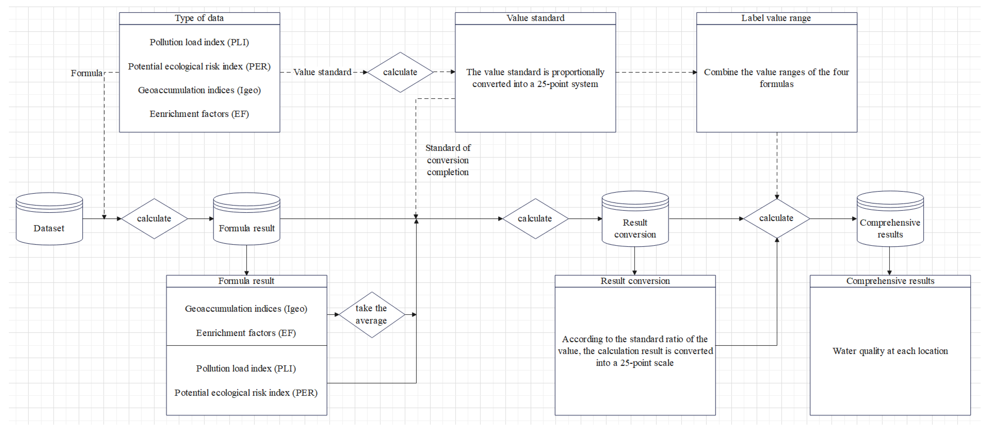Figure 1 illustrates the overall process of data labelling. Firstly, we compute the four indicators in accordance with their specifications. Among these results, Igeo and EF are calculated for each element in the water in the area, while PLI and PER are a comprehensive evaluation of all elements in the area. Because the number of levels among each indicator is not the same, it is necessary to systematically merge the label intervals among indicators.

According to standard text descriptions of Igeo, EF, PLI, and PER, we use the following formulas to transform each indicator into a 25-point scale.

For geoaccumulation indices (Igeo), the merger criteria are as follows:

$$f_{\mathrm{score}}\left(x_{\mathrm{Igeo}}\right)=\left\{\begin{array}{cc}0\hfill & \mathrm{if}{x}_{\mathrm{Igeo}}<0,\hfill \\ 5x\hfill & \mathrm{if}0\le x_{\mathrm{Igeo}}\le 5,\hfill \\ 25\hfill & \mathrm{if}{x}_{\mathrm{Igeo}}>5.\hfill \end{array}\right.$$

(1)

For the enrichment factors (EF), the merger criteria are as follows:

$$f_{\mathrm{score}}\left(x_{\mathrm{ef}}\right)=\left\{\begin{array}{cc}0\hfill & \mathrm{if}{x}_{\mathrm{ef}}<2,\hfill \\ \frac{25(x-2)}{38}\hfill & \mathrm{if}2\le x_{\mathrm{ef}}\le 40,\hfill \\ 25\hfill & \mathrm{if}{x}_{\mathrm{ef}}>40.\hfill \end{array}\right.$$

(2)

For the pollution load index (PLI), the merger criteria are as follows:

$$f_{\mathrm{score}}\left(x_{\mathrm{pli}}\right)=\left\{\begin{array}{cc}0\hfill & \mathrm{if}{x}_{\mathrm{pli}}<1,\hfill \\ \frac{25(x-1)}{4}\hfill & \mathrm{if}1\le x_{\mathrm{pli}}\le 5,\hfill \\ 25\hfill & \mathrm{if}{x}_{\mathrm{pli}}>5.\hfill \end{array}\right.$$

(3)

For the potential ecological risk index (PER), the merger criteria are as follows:

$$f_{\mathrm{score}}\left(x_{\mathrm{per}}\right)=\left\{\begin{array}{cc}0\hfill & \mathrm{if}{x}_{\mathrm{per}}<40,\hfill \\ \frac{25(x-40)}{280}\hfill & \mathrm{if}40\le x_{\mathrm{per}}\le 320,\hfill \\ 25\hfill & \mathrm{if}{x}_{\mathrm{per}}>320.\hfill \end{array}\right.$$

(4)

We add the pollution degree label to the dataset based on the total score of the above four indicators, as: score = 0 = A level (unpolluted), 0–16.8 = B level (light pollution), 16.8–54.48 = C level (moderate pollution) and >54.48 = D level (heavy pollution). The scoring ranges of the above four types of pollution degree labels are obtained based on the results of combining the original pollution assessment standards of the above four environmental indicators into four grades artificially.

In fact, after the items in the dataset are calculated, the result does not contain D level (heavy pollution) data, and there is no data source for training the model, so the C level and D level are merged. When the score is greater than 16.8, all are C level.

4.2. Data Imputation

The data we collected has a large percentage of missing data, around 53%, which is problematic for the data-driven machine learning model. Therefore, a well-performing data imputation method is necessary to standardise and clean them to enhance the performance of machine learning models. We design an experiment to examine the efficiency of different imputation models, which includes: (i) simple imputation, (ii) k-nearest neighbour (KNN) imputation, (iii) singular value decomposition (SVD) imputation, and (iv) iterative imputation.

In our experiment, we select a dataset as the target domain. Then, experimentally, we evaluated the performance of various imputation methods. We performed the imputation methods under different missing rates and repeated the experiment ten times to obtain a statistically significant result. We randomly drop values with a missing rate ranging from 0.35 to 0.65, with an increment step of 0.05. Then we compared the mean of the symmetric mean absolute value (SMAPE) between the imputed and the actual values. The highest performing imputation method is selected in this research.

Tables 2 and 3 illustrate the performance differences in-between several data imputations methods. Simple imputation refers to using the mean across each feature column to fill missing values. Data standardisation refers to rescaling the value of each feature to the same scale to let all features contribute equally to the developed model. Several ways to standardise include min and max normalisation, z-score standardisation, and centralisation. Standardisation rescales the value into zero means and one unit standard deviation. Normalisation is to rescale the value into 0 and 1. Centralisation is to rescale the value to be centred at 0.

In classification and clustering algorithms, z-score standardisation performs when the distance is calculated to measure the similarity, or dimensionality reduction technologies, such as principal component analysis (PCA), are applied. In our dataset, the models we propose to develop, such as support vector machines (SVM) and KNN, highly rely on distance calculation, so we adopt the z-score standardisation technique.

4.3. Machine Learning Model Developing

The choice of the machine learning algorithm enables this study to obtain the water quality and pollution situation of a certain place in a timely and accurate manner, and the rapid and accurate prediction of water quality is helpful to water quality regulation to a large extent. In addition, this study uses the data imputation method in combination with the machine learning algorithm to tack the typical data scarcity issue with water sediment datasets, so that our model would assist in precisely assessing water quality based on potentially incomplete real-world data.

The machine learning models we adopted in this research are Logistic Regression, Naive Bayes, Decision Tree, KNN, SVC, and MLPClassifier. Logistic regression is a linear regression plus a sigmoid function that can convert numeric prediction into categorical outcomes. The Naive Bayes classifier is a classification technique that uses Bayes’ Theorem as its underlying theory. It assumes that all the predictors are independent; that is to say, all features are unrelated and do not have any correlation. KNN is the k-nearest neighbour classifier. It calculates the distances between the data entry to be predicted and other data entries, then votes for the most frequent label among k closest number of data entries to predict the label of the target entry (k is a hyperparameter that needs to be tuned during model training). SVC stands for support vector classifier. There is no required assumption on the shape of features, and no parameters need to be tuned. It generates the ’best fit’ hyperplane that divides or categorizes the samples. MLPClassifier is a multi-layer perceptron (MLP) that trains a neural network using a backpropagation algorithm.

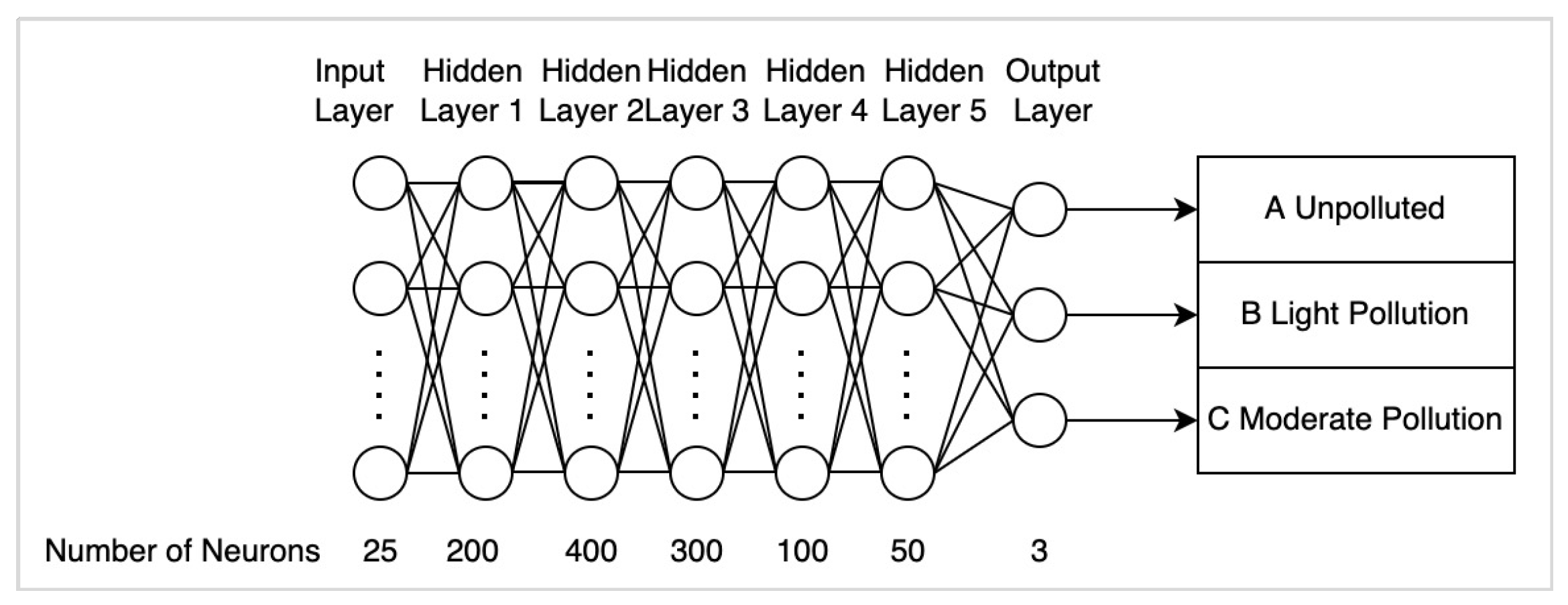
In addition to MLPClassifier, we build a fully connected deep neural network (DNN) and tune the hyperparameters to find a DNN model with the highest predicting accuracy. DNN is an artificial neural network with many hidden layers between its input and output layers. The number of neurons in the input and output layer is the same as the number of data entries and different labels in the dataset. A weighted sum plus a bias is applied to all the neurons in the previous layer. A non-linear function is used to change its linearity. Then the calculated value works as the input value of neurons in the next layer. The weight of each neuron will not be updated through the backpropagation algorithm until the loss function is minimized. Then the latest weight, together with other parameters, form the architecture of the DNN model.

Table 1. Brief description of each machine learning model.

Model	Description
Logistic Regression	A traditional statistical method to predict the classes via fitting regression curves
Naive Bayes	A model that applies Bayes’ theorem for prediction with a strong assumption of conditional independence
Decision Tree	Uses a tree-like model to divide the input into various classes via splitting the input into a series of related choices
KNN	A straightforward non-parametric approach to use distance metric for making classification based on nearby data
SVC	A support vector machine that perform classification by creating a hyperplane that separate the datapoints
MLP	A simple feed forward neural network that can be trained by back propagation

provides a brief summary of each machine learning models.

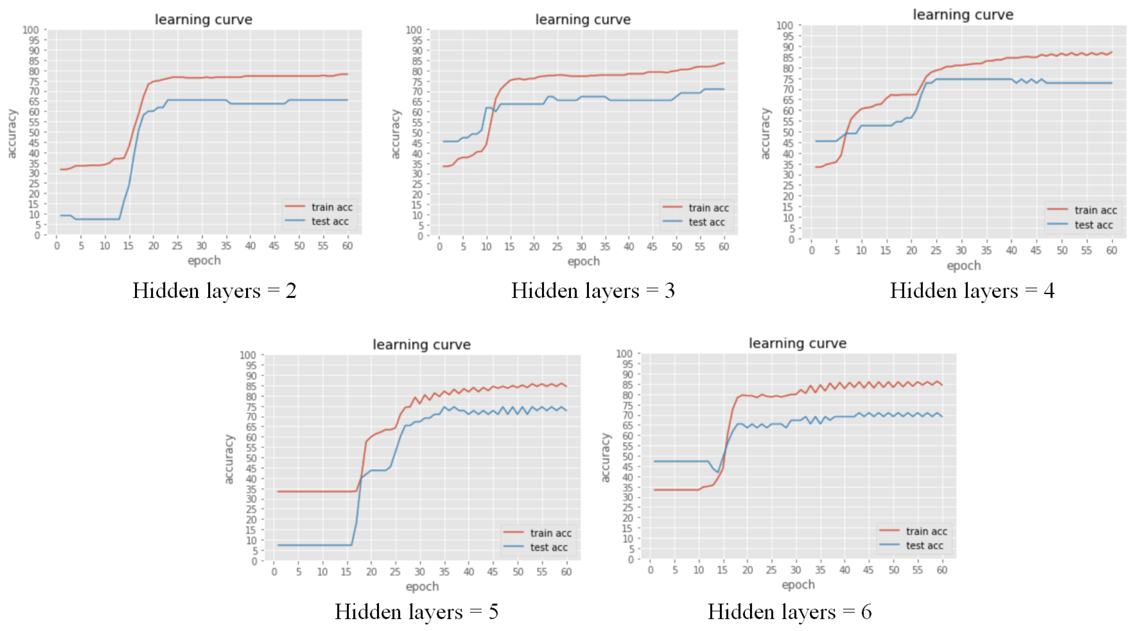
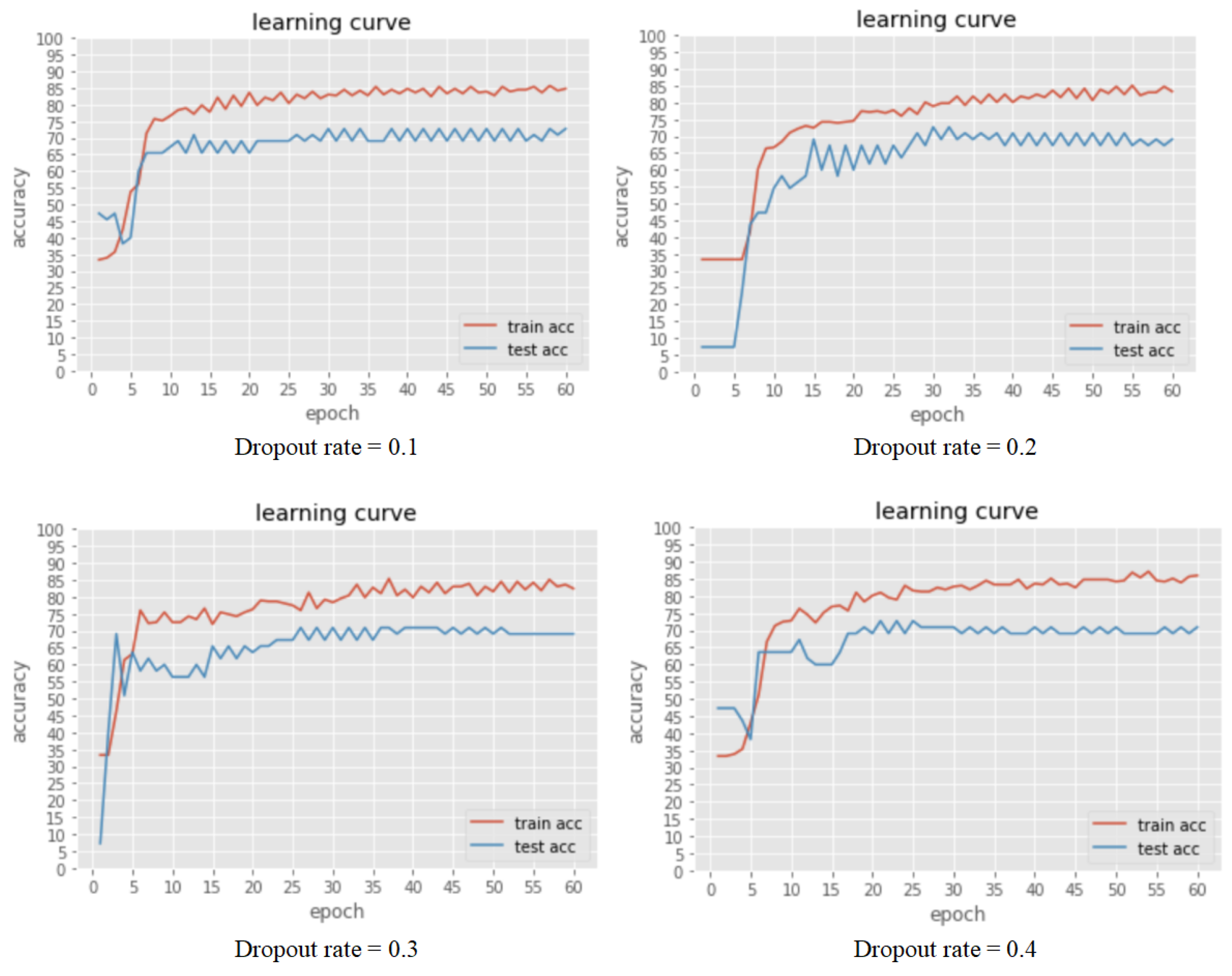
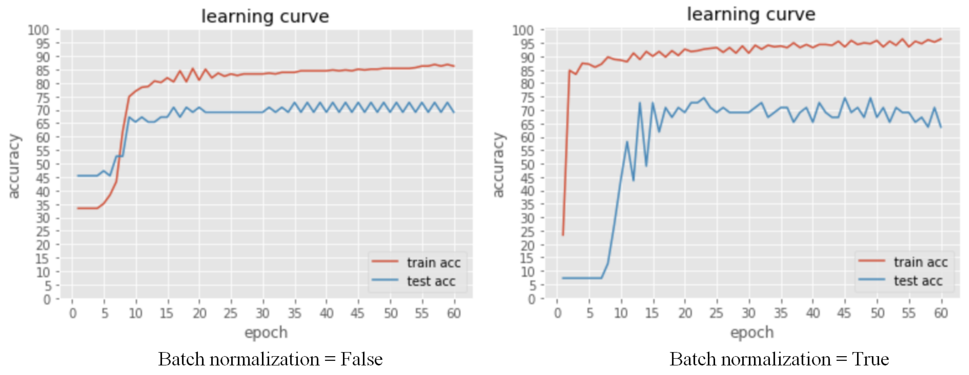
Parameter tuning is the most crucial task during DNN model development. In this project, we use predicting accuracy to examine the efficiency of different parameters. Typical parameters include the number of hidden layers, the number of neurons in each layer, the activation function, the dropout rate, the batch normalization, the epoch, and the gradient descent method. We first tune the number of hidden layers and then use the best number of hidden layers to tune the number of neurons in each layer. Then, we tune the dropout rate and evaluate batch normalization’s effectiveness.

Logistic regression is one of the straightforward and easy-to-interpret algorithms in machine learning, so it is used as the benchmark model in our comparison. Prediction accuracy and F1-score will be compared between those models. Details of machine learning model accuracy evaluation methods will be discussed in the subsequent section.

4.4. Data Collection

The dataset used in this research was collected from some authoritative websites and combined by the following six datasets from various sources.

• Dataset I was collected by Jahan and Strezov (2018). Using Ekman grab sampler, they collected sediment samples from three different locations at each of the six ports of Sydney, Jackson port, Botany port, Kembla port, Newcastle port, Yamba port, and Eden port, and obtained the content data of 42 different substances in sediments at different sampling points [3].
• Our Dataset II comes from Perumal et al. (2019), which includes surface sediments from 24 different locations in the areas affected by different anthropogenic activities in the coastal area of Thondi using Van Veen grab surface sampler, and measured the grain size, organic substance, and heavy metal concentration of surface sediment samples [15].
• Dataset III was collected by Fan et al. in 2019. Using the Bottom Sediment Grab Sampler, they collected 70 surface sediment samples in Luoyuan Bay, northeast coast of Fujian Province, China, and measured the concentrations of eight heavy metals, V, Cr, Co, Ni, Cu, Zn, Cd, and Pb, in the sediment samples [16].
• Dataset IV was collected by Constantino et al. (2019) at nine different sampling points in the Central Amazon basin. During the dry season, they collected sediment samples with a 30 by 30 cm Ekman–Birge dredger and measured the concentration of different metals in sediment samples [17].
• Dataset V was collected in a polygon along the Brazilian continental slope of the Santos Basin, known as the São Paulo Bight, in an arc area on the southern edge of Brazil, to obtain Dataset V [18].

4.5. Data Augmentation

Our labelled dataset is highly imbalanced, with label ‘A’ accounting for 43%, label ‘B’ accounting for 51%, and label ‘C’ accounting for 6%. In an imbalanced dataset, the predicting accuracy (the number of correctly predicted samples/the total number of samples) will become ineffective. This is because the positive samples in an imbalanced dataset occupy a large percentage, and the accuracy score will become high even if none of the negative samples is successfully predicted. When the ratio of two groups of samples exceeds 4:1, the imbalance problem will be severe.

There are three standard methods for dealing with an imbalanced dataset: (i) resampling, (ii) over-sampling, and (iii) under-sample. Our original data entries are small, so we choose over-sampling, synthesising data entries for the minority label classes. This process is also known as data augmentation. The most straightforward augmentation technique is picking a small number of samples at random, then making a copy and adding it to the whole sample. However, if the feature dimension of the data is small, simple extraction and replication will lead to over-fitting easily. We adopted a new augmentation method called Synthetic Minority Over-sampling Technique (SMOT). SMOT is to find K numbers of neighbours in P dimensions and then multiply each index of the K neighbours by a random number between 0 and 1 to form a new minority class sample. SMOT can introduce some noise to the synthesised samples to avoid the problem of overfitting.

4.6. Evaluation

Data imputation: evaluating the appropriate data imputation approach is an essential process to address the issue with missing data which is common among sediment data. We have selected four state-of-the-art approaches as the candidate methods. The designed experiment calculated the average accuracy of different imputation methods under different missing rates. SMAPE is used to evaluate the models’ performance. Using SMAPE instead of MAE or RMSE helps to account for the magnitude differences between features. In addition, accuracy and F1-score are used to examine the performance of the models.

5. Results

5.1. Data Imputation Results

The SMAPE value of different missing data imputation methods is shown in

Table 2. The SMAPE score (mean and standard deviation) by using mean imputation and SVD imputation.

Imputation Method	Data Missing Rate
	0.35	0.4	0.45	0.5	0.55	0.6	0.65
Mean Imputation	115.42 ± 3.45	111.44 ± 3.11	112.06 ± 4.81	111.58 ± 6.87	108.61 ± 7.24	110.51 ± 5.47	109.02 ± 6.24
SVD Imputation	112.63 ± 4.80	114.08 ± 4.08	112.91 ± 5.99	111.97 ± 4.06	114.57 ± 7.96	106.98 ± 6.61	106.30 ± 6.68

, illustrated by its mean and standard deviation.

Table 3. The SMAPE score (mean and standard deviation) by using kNN imputation and iterative imputation.

Imputation Method		Data Missing Rate
		0.35	0.4	0.45	0.5	0.55	0.6	0.65
	$k=5$	90.77 ± 7.31	98.49 ± 10.10	97.63 ± 4.98	96.74 ± 6.74	98.85 ± 4.60	102.70 ± 5.32	104.09 ± 4.83
	$k=7$	93.49 ± 5.92	96.89 ± 5.93	101.57 ± 4.79	103.57 ± 9.84	112.02 ± 6.40	109.42 ± 7.54	107.64 ± 7.20
	$k=9$	100.12 ± 8.11	100.09 ± 8.82	109.13 ± 9.04	111.02 ± 4.35	109.28 ± 3.34	108.88 ± 8.14	105.98 ± 8.01
	Bayesian Ridge	114.92 ± 7.78	116.46 ± 6.56	122.05 ± 5.15	119.76 ± 6.09	123.83 ± 5.28	123.91 ± 6.43	123.25 ± 7.18
Iterative Imp.	Decision Tree	60.11 ± 5.19	62.22 ± 3.31	64.27 ± 3.68	66.78 ± 6.40	68.75 ± 5.10	70.34 ± 9.64	80.04 ± 9.06
	$n=5$	60.25 ± 4.00	61.84 ± 2.37	58.40 ± 33.35	65.05 ± 5.44	63.36 ± 3.36	66.88 ± 3.27	70.91 ± 7.69
	$n=20$	62.46 ± 2.72	64.33 ± 5.98	64.98 ± 5.55	66.38 ± 4.25	67.52 ± 4.89	70.20 ± 3.13	77.58 ± 5.22
	$n=50$	62.13 ± 5.94	65.99 ± 6.18	65.94 ± 4.49	68.34 ± 4.50	71.76 ± 3.32	71.00 ± 5.41	76.57 ± 6.59

shows the iterative imputation using different tree algorithms with a different number of trees. Figure 2 gives a clear comparison of different imputation methods with simple imputation as the benchmark. The green line indicates that the SMAPE of simple imputation is 111.58. Any column above the green line means that the method performs better than simple imputation and vice versa.

Table 4. The mean and standard deviation of SMAPE in ExtraTree with different tree numbers.

Missing Rate (%)	0.35	0.4	0.45	0.5	0.55	0.6	0.65
Iterative Imputation with Extra Tree Estimator
n = 5	60.25 ± 4.00	61.84 ± 2.37	58.40 ± 33.35	65.05 ± 5.44	63.36 ± 3.36	66.88 ± 3.27	70.91 ± 7.69
n = 20	62.46 ± 2.72	64.33 ± 5.98	64.98 ± 5.55	66.38 ± 4.25	67.52 ± 4.89	70.20 ± 3.13	77.58 ± 5.22
n = 50	62.13 ± 5.94	65.99 ± 6.18	65.94 ± 4.49	68.34 ± 4.50	71.76 ± 3.32	71.00 ± 5.41	76.57 ± 6.59

illustrates the mean and standard deviation of SMAPE in ExtraTree with different tree numbers.

5.2. Deep Learning Model Tuning Results

5.2.1. Tuning the Number of Hidden Layers

Figure 3 illustrates the prediction accuracy of the train and test dataset under different numbers of hidden layers ranging from 2 to 6, increased by 1. The test accuracy with two hidden layers equals 0.65, increases to 0.75 when hidden layers are 4 and 5, then drops to 0.70 with six hidden layers. The training accuracy for 4 and 5 hidden layers is 0.87 and 0.85, separately. Hence, the five hidden layers prevail over four hidden layers due to less overfitting.

5.2.2. Tuning the Dropout Rate

From the previous tuning process, we find an overfitting problem during model development. We tune the dropout rate ranging from 0.1 to 0.4, which is increased by 0.1 to lessen the accuracy gap between train and test datasets. Figure 4 shows that the performance difference between different dropout rates is similar, but the 0.2 dropout rate has a slight advantage around 30 epochs, where the training accuracy is 80, and the testing accuracy is 0.75.

5.2.3. Tuning the Batch Normalization

Batch normalization is another technique used to solve the overfitting problem. The criterion is whether to adopt batch normalization after each hidden layer or not. The left-hand side graph in Figure 5 indicates not using batch normalization, and the right-hand side graph indicates using batch normalization. Using batch normalization performs worse than not to use.

Architecture of the final DNN model: from above model tuning, we finally choose the DNN model with one input layer, five hidden layers, and one output layer. The number of neurons in each layer is (25, 200, 400, 300, 100, 50, 3). There is no dropout or batch normalization in this model. The architecture is shown in Figure 6.

5.3. Model Development Results

The values of the accuracy score and F1-score corresponding to different trained models are shown in Figure 7. It can be seen that SVC, NuSVC, and DNN models have the highest performance on the metric of accuracy, and their corresponding accuracy classification score is 0.75. In contrast, it is noted that the NuSVC model has the highest performance on the metric of F1-score, and its corresponding F1-score is 0.76. As mentioned earlier, the above metrics were used to evaluate the prediction accuracy of a model. The larger the value of the above metrics, the higher the accuracy of a model.

6. Discussion

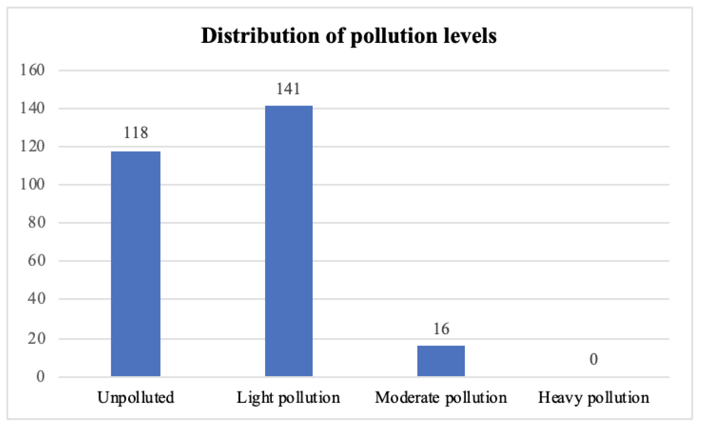
Labelling the data with the pollution level is essential in this research. The labelling standard was made for research, so it is essential to consider its reliability. This is because our research result will be meaningless if the label is unreliable. No specific performance metrics can be chosen to evaluate that process about labelling the level of pollution, but the distribution of the level of pollution is consistent with our background research. According to Figure 8, the distribution of different pollution levels mainly focuses on polluted and light pollution, which accords to real-life situations. There is no severe pollution which is reasonable since the government will control that situation. In addition, the algorithm we chose to calculate the level of pollution reflects the pollution degree values of metal concentration of sediments more.

From our research, there are a few detailed applications to various areas. Firstly, a practical system to evaluate the level of pollution is achieved. As mentioned before, it is believed that the system to estimate the level of pollution using indexes is entirely usable for a simple estimation. Although the guideline of labelling different data into four levels of pollution was created in this research, its reasonability is solid. The comprehensive evaluation of water quality is complicated, and it will consider many factors, including some compounds that were not included in this research [17]. The guideline established in this research followed the process of water quality guidelines. In many situations, the measurement of all various compounds cannot be performed due to the complexity. Our guideline, which can generate pollution labels for sediment samples by the mental concentration in water sediments, is a good choice for simple and preliminary evaluation.

6.1. Missing Data Imputation

In addition, we experimented to find the best methods for missing data imputation. The experiment result of which method will be better for imputation can be referenced by experiments with a small dataset having a large percentage of missing data. Similar situations can reference the result. In the case of this research, the rate of missing data is about 53% which is too high to take standard methods of missing data imputation, such as filling the missing data with mean, especially when the dataset is relatively small.

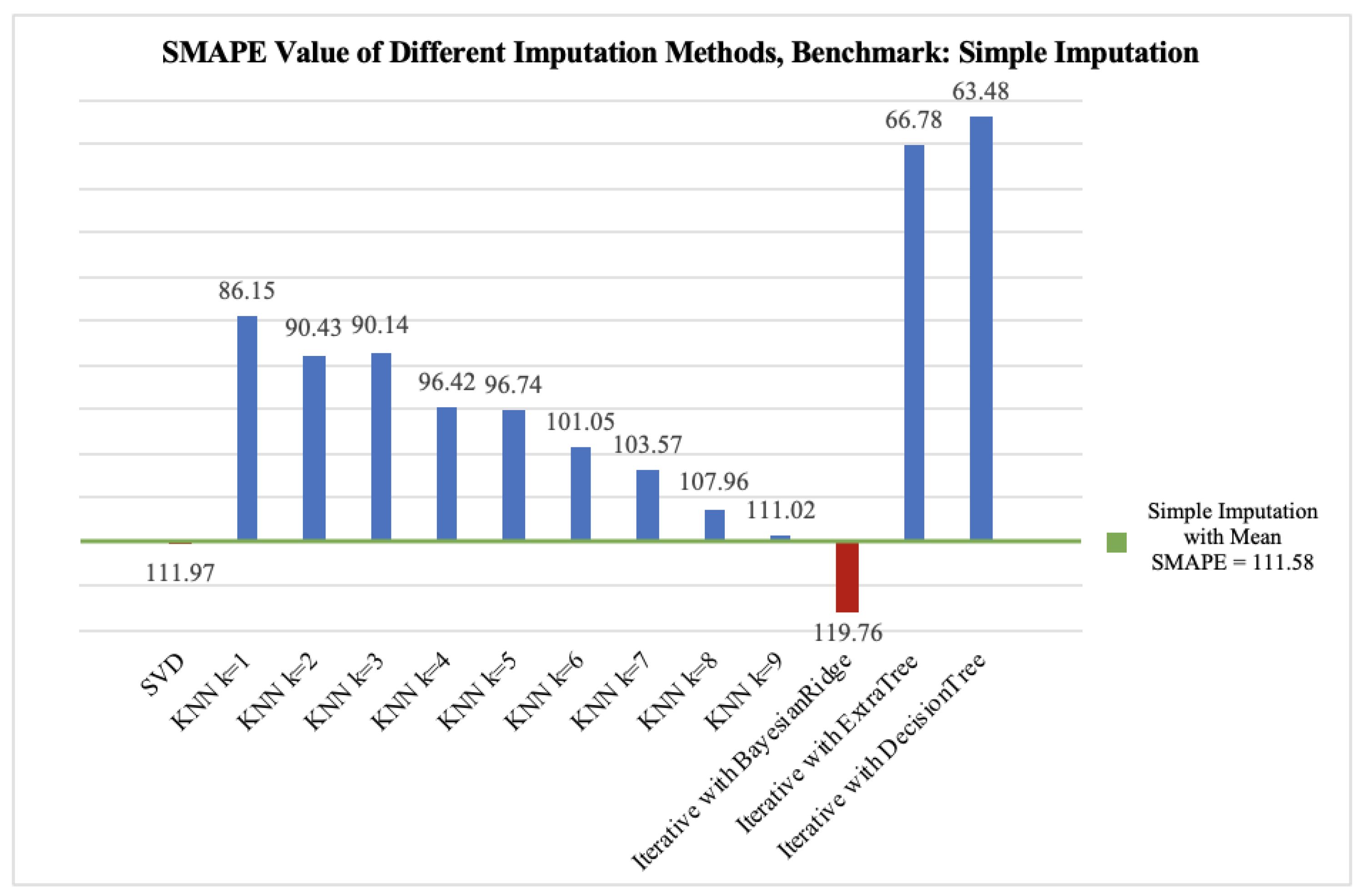
As the missing rate in our dataset is around 53%, we focus on the SMAPE values of different missing data imputation methods under the 0.50 missing data rate. A lower score in SMAPE value implies a better imputation performance. All the imputation methods perform better than simple imputation except iterative imputation with BayesianRidge and SVD. SVD performs slightly worse than simple imputation. Iterative imputation with extra trees has the best performance. Notably, the number of trees (n) in extra tree regression can be tuned as well, so we tried n equals 1, 5, 10, 20, and 50, and the outcome in Section VI-A clearly shows that the SMAPE of iterative imputation with extra trees is the lowest when n equals 10. In conclusion, the selected imputation method in this project is iterative imputation with the extra tree algorithm (n = 10) as the estimator.

6.2. Model Developing

From our result, it can be deduced from the algorithm calculating the pollution level and variable importance plot that Fe, Cu, Zn, Co, Mn, Se, and Ni are the metals that most affect the quality of sediments. The practical significance of this result is that the government will know the concentration of what kind of metals in sediment should be strictly controlled.

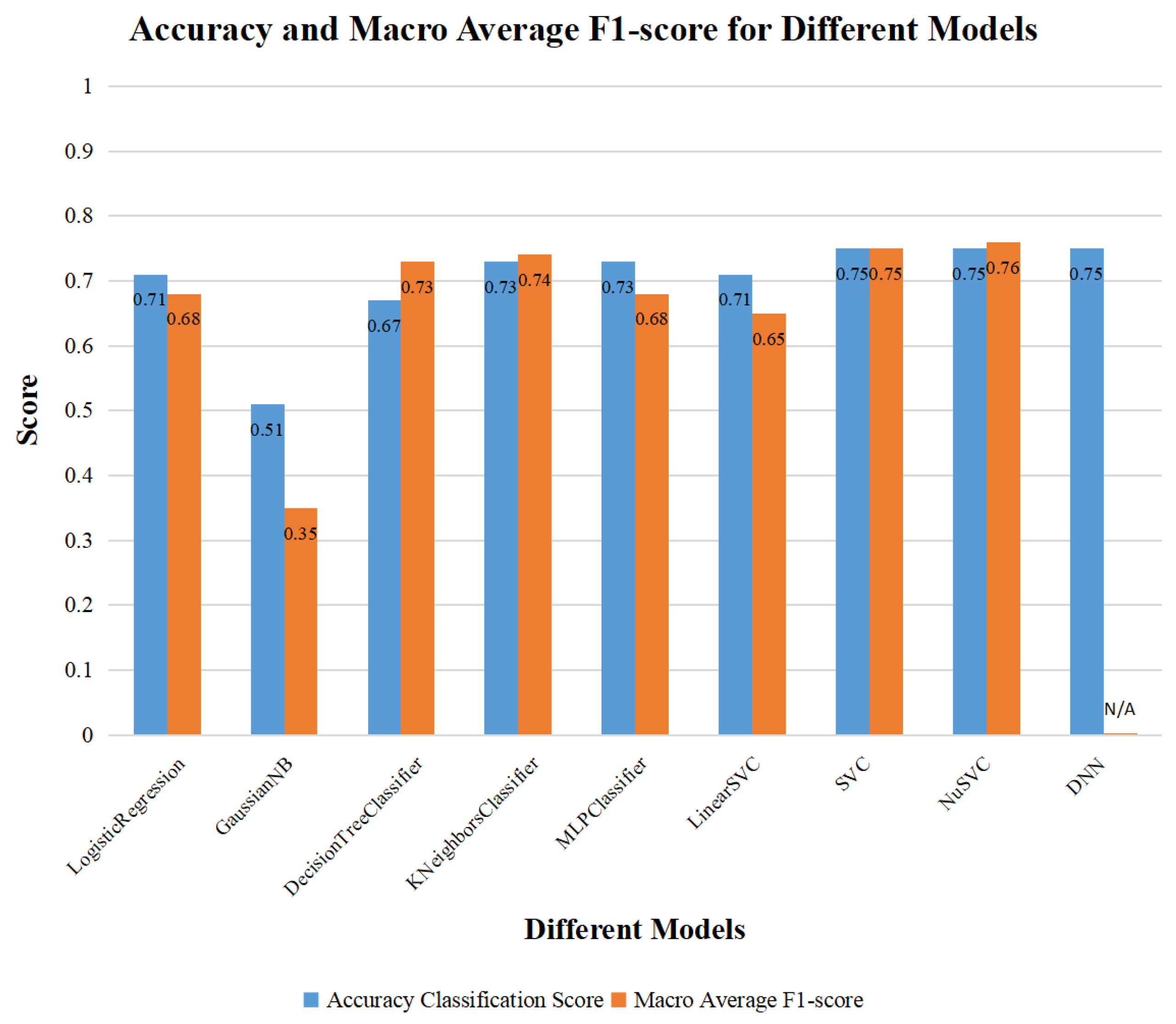
According to Section VI-C, the accuracy scores of NuSVC and DNN models are about 0.75. In other words, the percentages of correct prediction classification of NuSVC and DNN models are similar. However, the F1-score of DNN model is unavailable, as is mentioned in Section IV-D, it is difficult to compare the performance of NuSVC and DNN through that. Since the available dataset collected in this research is too tiny, the difference in training speed between NuSVC and DNN models is not apparent. In addition, there is no complex hyperparameter adjustment process in training the NuSVC model compared with DNN model.

7. Conclusions

Water sediment is an essential part of the ecological environment, and its physical and chemical properties will affect biological integrity. Therefore, investigating and studying water sediments is one of the ways to detect the quality of the water environment. This research uses machine learning technology to evaluate the quality of the water-sediment samples taken to evaluate the quality of seawater samples at different locations and depths and provide adequate information to evaluate the quality of the nearby water environment.

We propose a unified framework for introducing the predictive capability of modern machine learning techniques into water and sediment analysis. Our framework provides a systemic approach to evaluate the most appropriate data imputation methods to tackle data scarcity and missing data issues, which are typical in existing studies. Our final model archives state-of-the-art performance across other models to classify water pollution level.

Future Work

Based on the above limitations, two improvement works can be done in the future.

On the one hand, regarding the accuracy of the output results and the overfitting problem encountered in model training, the ultimate reason for the limitations is related to the dataset. Therefore, future work will focus on expanding the capacity of the dataset and improving its quality. Specific conceivable ways include:

(1)

Getting the authorisation of the data set or purchasing the relevant dataset by getting in touch with the official agency or authority.

(2)

If necessary, try to cooperate with relevant experts or research groups, hoping that they can assist us in testing more water quality data.

(3)

For the existing data, improve the quality of data pre-processing as much as possible and reduce redundant and invalid data.

On the other hand, the effectiveness of the label will be the focus of consideration since the artificially generated label may lack authority. Therefore, in future work, it is necessary to consult more relevant authoritative organisations and environmental science scholars to obtain a more mature label method.