LoRaWAN Network Downlink Routing Control Strategy Based on the SDN Framework and Improved ARIMA Model

Abstract

In order to improve the downlink communication performance of the traditional LoRa wide area network (LoRaWAN), a LoRaWAN downlink routing control strategy based on the software defined networks (SDN) framework and the improved auto-regressive integrated moving average (ARIMA) model is proposed. The SDN architecture is used to monitor the network traffic, and the link bandwidth occupancy rate is calculated based on the monitored downlink traffic. Taking into account the impact of data volatility on the accuracy of the prediction results, the Savitzky–Golay (S–G) smoothing filter and the sliding window method are introduced for data pre-processing. Stationarity processing is carried out for the time series data in the window, and the ARIMA model is developed to predict the downlink bandwidth occupancy rate. The triangle module operator is then used to incorporate multiple path parameters to finally calculate the selectivity of different paths, and the optimal path for LoRaWAN downlink communication is then provided. Simulation and experimental results show that the root mean square error of the improved ARIMA prediction model is reduced by 87% compared with the standard ARIMA model. The proposed routing control strategy effectively reduces the service transmission delay and packet loss rate. In the LoRaWAN test environment, as the downlink load rate increases, the average link bandwidth occupancy rate of this solution increases by 12% compared with the traditional method.

1. Introduction

With the development of Internet of Things (IoT) technology, low-power wide-area networks (LPWAN) technologies are able to fill the gap between short-range wireless multi-hop ad hoc networks and cellular networks [1]. Wireless sensor network technologies [2,3] have become an important research area. Currently, LPWANs are suitable for multiple IoT applications, such as smart city [4], smart energy [5,6], environmental monitoring [7] and other fields. One of the main technologies of LPWAN is long -range wide-area network (LoRaWAN) [8], which is an open standard framework that allows long-range communication between thousands of low-power-consumption battery-powered devices and a continuously online gateway with a cellular structure. Research into LoRaWAN communications can be mainly divided into two categories: uplink communication and downlink communication. Related research of uplink communication mainly includes the network access reliability of equipment, the performance optimization of frequency hopping transmission, the quality of service of the LoRa network, the physical performance of the LoRa signal, etc. In [9], the reliability of the terminal equipment network transmission mechanism and the network communication delay in LoRaWAN uplink communication are discussed. In [10,11,12], the dual key activation update method is used to ensure the security of physical devices in the LoRaWAN network. The LoRaWAN uplink communication research helps to solve the reliability problems of stable network access for terminal equipment and data collection. However, the reply and message confirmation of the network server are usually ignored in such types of research. As for downlink communication, the transmission of business information such as control instructions and interactive data is usually involved, which makes the downlink communication an important part of the LoRaWAN network. It is of great significance to develop the optimal LoRaWAN network downlink routing control strategy to construct the high-performance and high-reliability LoRaWAN network.

In the downlink communication of the LoRaWAN network, transmission delay and packet loss rate are important parameters to evaluate the downlink communication service quality. In [13,14], it is shown that the downlink communication performance is usually limited by the arrival rate, the retransmission times, and the data rate of uplink data. It is proposed to employ downlink channel monitoring, the cyclic broadcast, and the multicast method to improve the downlink communication performance. However, most of these studies try to improve the communication performance based on the optimization of the communication polling mechanism. The routing control is hardly studied.

It is known that in LoRaWAN communication, data control and forwarding are closely related. With the increase of the downlink load rate, communication congestion is very likely to be induced if the proper routing control is missing.

In recent years, software defined networks (SDN) technology has evolved into a flexible strategy for ensuring heterogeneous networks support a wide range of application requirements, as shown in Table 1.

Table 1. The related work of the SDN.

Reference	Contribution	Exiting Problem
[15]	The link delay information based on the SDN is used to select the optimal transmission route	the time series regression analysis for the data processing is not constructed
[16,17]	The resource balancing algorithm and the routing reconstruction model of SDN is discussed to reduce the delay of service data transmission
[18,19,20,21]	The SDN framework provides a new feasible solution for the routing optimization of downlink communication in LoRaWAN network

In the process of data downlink transmission, when the network is overloaded or congested, by applying the proper routing control strategy, the resource allocation mechanism in SDN offers the possibility to ensure highly efficient network communication. It is known that the bandwidth occupancy rate of the downlink communication link is a system with periodic dynamic changes [22,23]. It is needed to construct the time series regression analysis for the data processing. In this paper, the auto-regressive integrated moving average (ARIMA) time series algorithm is developed to model and analyze the LoRaWAN downlink bandwidth occupancy. Aiming to solve the problems of high packet loss rate and large transmission delay in the existing LoRaWAN network downlink communication, a LoRaWAN network downlink routing control strategy is proposed based on the SDN framework and the improved ARIMA model. The SDN framework is used to establish the downlink routing model of the LoRaWAN network to realize the monitoring of the network status in the downlink routing process. In order to improve the prediction accuracy of the existing ARIMA model, an improved ARIMA model by combining the Savitzky–Golay (S–G) filtering and the sliding window method is proposed to improve the data stationarity.

• According to the reconstructed data, an ARIMA-based link bandwidth occupancy rate prediction model (LBOP-ARIMA) is established, and the link bandwidth occupancy rate is predicted.
• Then, according to the triangular modulus operator, parameters such as the transmission delay of the network downlink communication route, and the routing bandwidth occupancy rate at time t and time t + T are integrated, and different routing degrees are calculated.
• The downlink routing control is simulated on the Mininet platform, and the communication performance of different routing control strategies is compared. On this basis, the LoRaWAN network application platform test is then built up, and the reliability of the downlink communication is verified for the proposed scheme.

The paper is organized as follows: The LoRaWAN network downlink communication is introduced in Section 2. In Section 3, the LBOP-ARIMA model is proposed. LoRaWAN downlink routing control strategy is presented. Experiment and analysis are carried out in Section 5. The conclusions are given in Section 6.

2. LoRaWAN Network Downlink Communication

2.1. Downlink Communication Mechanism Based on the SDN Framework

In this paper, a LoRaWAN downlink communication mechanism is proposed by combining the software defined network framework and the improved ARIMA model. The proposed downlink routing mechanism is shown in Figure 1. The routing mechanism is mainly composed of three parts, the host, the transport layer and the terminals. The link layer discovery protocol (LLDP) is developed for the host to enable the server to quickly and accurately set up the global topology of the downlink routing of the LoRaWAN network and the network status parameters. The SDN controller at the transport layer collects and manages the network status according to the traffic information, and then formulates the corresponding downlink communication routes. The link bandwidth occupancy rate prediction module sends out the received downlink bandwidth occupancy rate at time t into the time series ARIMA model for training, and the occupancy rate is predicted for time t + T, where T represents the sampling point. The selectivity Q of different routes are calculated from the routing calculation module based on the triangle module of fuzzy mathematics. According to the flow entries, data is transmitted to the LoRaWAN gateway by the SDN switch. Finally, the downlink data packet is transmitted to the terminal device by the LoRaWAN gateway. Routing protocols are applied between network server to SDN switches. The ARIMA link bandwidth occupancy prediction model (LBOP-ARIMA) in the SDN control layer is the core part of the routing mechanism. This mechanism takes advantage of the OpenFlow protocol to implement the real-time information exchange between the control layer and the gateway and separates the processes of data control and data forwarding, and thereby reduces the transmission delay and packet loss rate.

Figure 1. Gateway and server downlink communication protocol.

2.2. Downlink Routing Modeling Based on the SDN

The downlink routing model is developed to analyze the data packets downlink routing process of LoRaWAN based on the SDN framework. We assume the downlink routing model is represented as G = (V, L), where V = {v₁, v₂, …, v_i} is the switch node sets in the LoRaWAN downlink routing and $i$ denotes the different SDN switch numbers. The downlink route set is represented as L = {l₁, l₂, …, l_j}, where j refers to the number of each downlink route. A downlink routing model of LoRaWAN network based on the SDN framework is developed and the modeling topology is shown in Figure 2. The routing of the downlink communication is set up by the SDN controller to monitor the network operation status. The OpenFlow protocol is adopted, and the flow entries are developed for the data transmitting. The downlink communication data can only be sent and received on the port connected with the corresponding SDN switch.

Figure 2. The LoRaWAN downlink modeling topology based on the SDN framework.

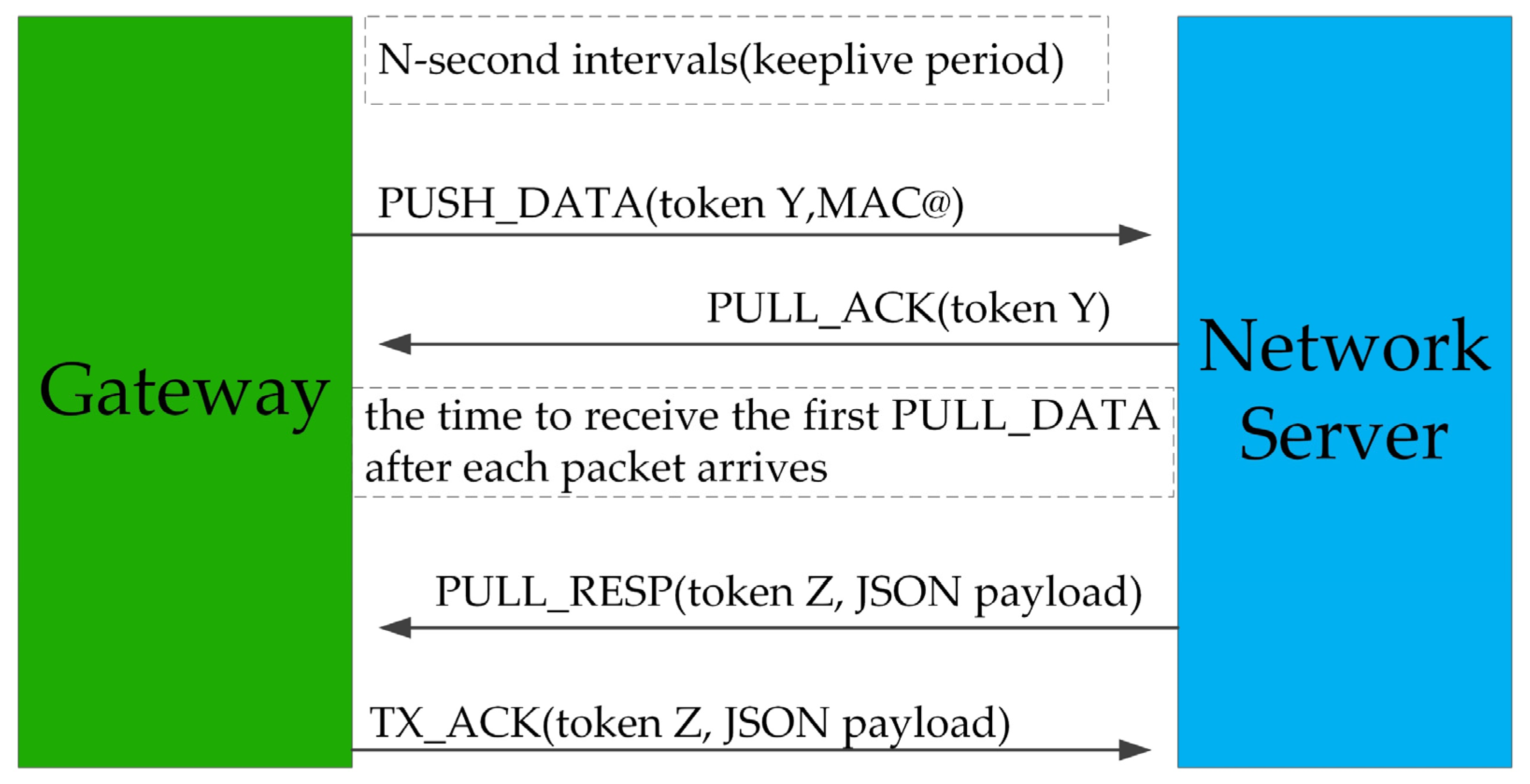
2.3. LoRaWAN Downlink Communication Protocol

The sequence interaction process of the downlink communication between the gateway and the server in the LoRaWAN network is shown in Figure 3. It is seen that the periodically transmit keepalive messages is needed to maintain the connection. PUSH_DATA messages are periodically sent out to inform the network server gateway of the UDP port number for receiving PULL_RESP data. The server responds to the PULL_DATA message with a PULL_ACK. Only after the interaction between the gateway and the network server is completed, the latest data can be delivered by the server. Application data is encapsulated in a JSON payload of PULL_RESP messages by the server. Lastly, the gateway decides whether to send a TX_ACK message to the network server according to the currently adopted LoRa gateway message protocol (GWMP) version. Before the network server sends data, it needs to confirm whether it has received the latest PUSH_DATA message. If the message is not received, a new PUSH_DATA needs to be sent out by the gateway.

Figure 3. Gateway and server downlink communication protocol.

PUSH_DATA and PULL_ACK are interactions that need to be completed before the server sends out data. The purpose is to ensure normal communication between the gateway and the service, and to keep the firewall of the gateway open. The sending period of the PULL_DATA message is set up by the gateway. In the downlink communication process, the network server calculates the modulation profiles (spreading factor, SF; code rate, CR; bandwidth, BW, etc.) of the downlink frame and the transmission timestamp in the downlink frame scheduling stage. When the internal clock reaches the downstream timestamp, the LoRaWAN gateway can only be programmed to leave one frame at a time. Therefore, downlink frames are buffered in a just-in-time queue. This hardware limitation exacerbates the problems caused by the half-duplex mode of the gateway and accelerates the duty cycle saturation process of downlink traffic, resulting in uneven link resource allocation in downlink routing and it is very likely to induce communication congestion.

2.4. Downlink Communication Status Parameters

The port parameter of the SDN switch and the status parameters of the flow entries in the LoRaWAN network are shown in Table 2. The status parameter $f_a(t)$ of the switch node $v_a$ from the flow entries and the port parameter $p_{a,q}(t)$ of the q port of the switch node $v_a$ are collected every ten seconds by the network traffic monitoring module, as shown in Table 2.

Table 2. The port parameter of the SDN switch and status parameters of the flow entries in the LoRaWAN.

Port Parameter	Sign	Explanation	Parameters of Flow Entries	Sign	Explanation
$p_{a,q}^1(t)$	rx_packets	number of packets received	$f_a^1(t)$	length	capacity of switch flow entries
$p_{a,q}^2(t)$	tx_packets	number of packets forwarded	$f_a^2(t)$	priority	matching order of flow entries
$p_{a,q}^3(t)$	rx_bytes	bytes received	$f_a^3(t)$	packet_count	number of packets forwarded
$p_{a,q}^4(t)$	tx_bytes	bytes forwarded	$f_a^4(t)$	byte_count	bytes forwarded
$p_{a,q}^5(t)$	rx_dropped	number of packets dropped while receiving	$f_a^5(t)$	duration_sec	duration of data flow
$p_{a,q}^6(t)$	tx_dropped	number of packets dropped while forwarding	$f_a^6(t)$	duration_nsec	extra time of data flow to live
$p_{a,q}^7(t)$	tx_errors	number of packets with errors while forwarding	$f_a^7(t)$	idle_ timeout	relative time to remove flow entries
$p_{a,q}^8(t)$	rx_frame_err	number of error frames when receiving	$f_a^8(t)$	hard_timeout	absolute time to remove flow entries
$p_{a,q}^9(t)$	rx_over_err	number of packets overflowed when receiving	_	_	_

In Table 2, $f_a^{\phi }(t)$ is defined as the status parameter of the $\phi$-type of $v_a$ from the flow entries at time t where $a,\phi \in N$, and $p_{a,q}^{\beta }(t)$ are defined as the status parameters of the β-type of the q port of $v_a$ from the flow entries at time t where $a,q,\beta \in N$. It can be seen from Table 2 that the status parameter $P_{a,q}(t)$ of the q port associated with node $v_a$ and the status parameter $F_a(t)$ from the flow entries can be described by the following equation.

$$\begin{gathered} P_{a,q}(t)=[p_{a,q}^1(t),p_{a,q}^2(t),\dots ,p_{a,q}^{\beta }(t)] \\ {F}_a(t)=[f_a^1(t),f_a^2(t),\dots ,f_a^{\phi }(t)] \end{gathered}$$

(1)

2.5. Downlink Communication Bandwidth Occupancy

Assuming that the link $l_j$ and the q port of the SDN switch node $v_a$ are connected to the g port of node $v_b$, the used bandwidth $b_j(t)$ of link $l_j$ at time t can be calculated as follows:

$$b_j(t)=\frac{p_{a,q}^4(t)-p_{a,q}^4(t-T)+p_{b,g}^4(t)-p_{b,g}^4(t-T)}{T}$$

(2)

In Equation (2), $p_{a,q}^4(t)$ is defined as the transmitted data of node $v_a$ at port q at time t, and $p_{b,g}^4(t)$ is defined as the transmitted data of node $v_b$ at port g at time t. Here, q, g are the port numbers of $v_a$ and $v_b$ $(q,g\in N)$.

In the process of downlink routing, $\max (B_j)$ is defined as the maximum bandwidth of the data flow that can be transmitted by link $l_j$, and the bandwidth occupancy rate of link $l_j$ at time t is calculated by the following equation:

$${\mu }_j(t)=\frac{b_j(t)}{\max (B_j)}$$

(3)

Here, Table 3 is set up to demonstrate the congestion level of the link bandwidth occupancy rate, in which $s_j(t)$ is used to represent the congestion degree of link $l_j$ at time t. The large value of s means the network tends to be congested.

Table 3. The congestion level of the link bandwidth occupancy rate.

${\mu }_j(t)$	${\mu }_j(t)$ Level	link Congestion Status	$s_j(t)$
0~0.6	1	no congestion	1
0.6~0.7	2	normal load	2
0.7~0.8	3	possible congestion	3
0.8~0.9	4	general congestion	4
>0.9	5	severe congestion	5

3. The LBOP-ARIMA Model

For the downlink communication mechanism, when the network traffic information is collected, the link bandwidth occupancy rate (LBOP) at time t can be calculated according to Equation (3). To develop the proper downlink communication routing strategy, the bandwidth occupancy rate at time t + T needs to be determined. Here, the LBOP-ARIMA model is developed to predict the occupancy rate at time t + T. The general auto-regressive integrated moving average model ARIMA model is characterized by the terms: p, d, q, where p is the order of the AR (auto-regressive) term, q is the order of the MA (moving average) term, and d is the number of differencing required to make the time series stationary. When the second-order difference sequence is used, the ARIMA (p, d, q) is described as following, in which parameter d is 2:

$$y_t={\epsilon }_t+{\displaystyle \sum _{i=1}^p{a}_i{y}_{t-i}+}{\displaystyle \sum _{i=1}^q{\beta }_i{y}_{t-i}+}c$$

(4)

where $y_t$ is defined as the time series value at time t, ${\epsilon }_t$ represents the random error at time t, $y_{t-i}$ is the observation value of the time series at time $t-i$, and $a_i$, ${\beta }_i$, and c are the regression parameters. The basic steps of establishing the ARIMA model are shown in Figure 4. Data acquisition and pre-processing is carried out in the first step. Secondly, time difference is used to check the smoothness of the time series data. Then, the p, and q terms are determined, and the model predictions are verified using the preset validation data set. The modeling process shown in Figure 4 is able to provide accurate predictions for data demonstrating periodicity and regularity. When there is data volatility involved, the process in Figure 4 may not be effective enough in providing accurate results and therefore must be improved.

Figure 4. The ARIMA modeling step.

3.1. The Savitzky–Golay Filtering

Compared with the standard ARIMA modeling process, the Savitzky–Golay smoothing filtering is proposed to be incorporated in the ARIMA model to take care of the data volatility problem. The main principle is to use a k^th order polynomial to fit the data points collected within a window of customized length. The S–G filtering is essentially a weighted average algorithm combined with a sliding window. The coefficient is obtained by fitting the data points in the sliding window with the least square method of a given high-order polynomial.

The multi-order weighting coefficient calculation is given here. The window length is set to be $n=2m+1$, and m is the integer constant (m ≥ 1). The sampling time is defined as $x=(x_1,x_2,\dots ,x_n)$, where $(x_1,x_2,\dots ,x_n)=\left(-m,-m+1,\dots ,0,\dots ,m\right)$. The objective of the (k − 1)^th degree polynomial is to fit the data points in the window. The fitting function is shown in Equation (5).

$$y={\partial }_0+{\partial }_{1}x+{\partial }_2{x}^2+\dots +{\partial }_{k-1}{x}^{(k-1)}$$

(5)

where ${\partial }_{k-1}$ is the (k − 1)^th coefficient and y represents the time series value at time x.

According to Equation (5), each measurement point is fitted to obtain n-related equations. To generate the solutions for the equations, it is necessary to set n as no less than k. Usually $n>k$ is selected, and the fitting parameter A is calculated according to the least square method, $A={[{\partial }_0,{\partial }_1,\dots ,{\partial }_{k-1}]}^T$,

$$\left[\begin{array}{c}{y}_{-m}\\ y_{-m+1}\\ ⋮\\ y_m\end{array}\right]=\left[\begin{array}{cccc}1& -m& \cdots & {(-m)}^{k-1}\\ 1& -m+1& \cdots & {(-m+1)}^{k-1}\\ ⋮& ⋮& ⋮& ⋮\\ 1& m& \cdots & m^{k-1}\end{array}\right]\left[\begin{array}{c}{\partial }_0\\ {\partial }_1\\ ⋮\\ {\partial }_{k-1}\end{array}\right]+\left[\begin{array}{c}{e}_{-m}\\ e_{-m+1}\\ ⋮\\ e_m\end{array}\right]$$

(6)

where $e_m$ represents the constant terms in the linear equations.

The least square solution $\stackrel{⏜}{A}$ of $A$ is:

$$\stackrel{⏜}{A}={\left(X^T·X\right)}^{-1}·X^T·Y$$

(7)

where $X=\left[\begin{array}{cccc}1& -m& \cdots & {(-m)}^{k-1}\\ 1& -m+1& \cdots & {(-m+1)}^{k-1}\\ ⋮& ⋮& ⋮& ⋮\\ 1& m& \cdots & m^{k-1}\end{array}\right]$, $Y={\left[y_{-m},\dots ,y_m\right]}^T$.

The model predicted or filtered value $\stackrel{⏜}{Y}$ of $Y$ is:

$$\stackrel{⏜}{Y}=X\cdot \stackrel{⏜}{A}=X\cdot {(X^T\cdot X)}^{-1}\cdot X^T\cdot Y=B\cdot Y$$

(8)

$$B=X\cdot {(X^T\cdot X)}^{-1}\cdot X^T$$

(9)

To run verifications, here the collected 12-h data set of network traffic status is trained and the time resolution is 10 s. The length of the sliding window is set when m = 5. The polynomial order is set as 3. The amount of downlink data in the specified window is calculated to obtain the sequence data of the bandwidth occupancy rate of link $l_j$. The original sequence is fitted and reconstructed. The above S–G smoothing filtering method is introduced, and the effect after processing is shown in Figure 5. It can be seen that the proposed strategy is effective at reducing the data fluctuation and thus improving the data stability.

Figure 5. Effect picture of pre-processing data by the sliding window method.

3.2. Model Parameter Selection

3.2.1. Determination of d

Before establishing the ARIMA model, the data stationarity of the original data series is checked. The autocorrelation function (ACF value) is described as follows:

$$ACF(k)={\rho }_k=\frac{Cov(y_t,y_{t-k})}{Var(y_t)}$$

(10)

Figure 6 shows the autocorrelation diagram of the bandwidth occupancy rate of link $l_j$. For a stationary sequence, there are usually two main types of autocorrelation plots: tailing and truncating. Truncation means that the autocorrelation coefficients are all 0 after a certain order delay. The tail indicates that the correlation coefficient varies not only in a non-zero state, but also shows a decaying trend. It can be seen from Figure 6 that the autocorrelation diagram of the sequence is neither tailing nor truncating. The time series downlink bandwidth occupancy rate demonstrates non-stationarity, which means the proposed ARIMA model is required to analyze and predict the link load data.

Figure 6. The autocorrelation diagram of the bandwidth occupancy rate of link $l_j$.

The difference calculation for the original sequence is used. The unit root test is adopted to verify the stationarity of the series. The test results obtained from the calculation are shown in Table 4. It can be seen from Table 4 that the absolute values of the T value of ACF of the original sequence are smaller than the absolute values corresponding with the rejection probabilities 1%, 5%, and 10%, which means the hypothesis that the sequence is non-stationary has to be accepted. The absolute values of the T value of the second-order difference series are greater than the absolute values of the 1%, 5%, and 10% levels, which means there is no single root in the second-order difference sequence, and the sequence has the characteristic of stability. Table 4 also shows that after the second-order difference, the acceptance probability is 0, which also proves that the second-order difference sequence is stable. It can be determined that in the ARIMA model, parameter d can be taken as 2.

Table 4. The ACF verification result.

	Type				Acceptance Probability (%)
	T	1%	5%	10%
Original sequence	−2.14	−3.86	−3.35	−3.21	32.56
First-order difference sequence	−3.75	−3.86	−3.35	−3.21	2.33
Second-order difference sequence	−23.68	−3.86	−3.35	−3.21	0.00

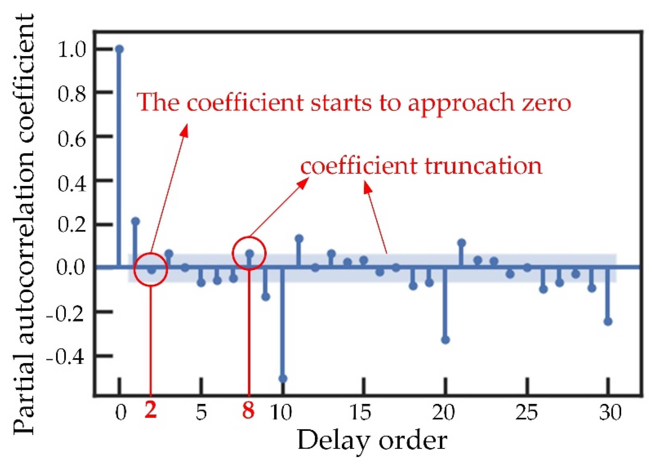
3.2.2. Determination of p, and q Value

There are typically two steps to choose p and q. The first step is to determine the approximate range of parameters which can be obtained according to the autocorrelation diagram and the partial correlation diagram of the d-order difference sequence. When the proper range is determined, the final p and q values can be obtained by comparing the modeling accuracy using different parameter combinations. The specific parameter determination method is shown in Table 5. Figure 7 and Figure 8 are the autocorrelation and partial autocorrelation diagrams of the second-order sequence of downlink traffic. It can be seen from Figure 7 that the autocorrelation coefficient truncation is observed after the second-order difference. So, q can be taken as MA (2), MA (3) or MA (4). Figure 8 shows that the partial autocorrelation coefficient truncation occurs after the eight-order difference, which means p can be taken as AR (2), AR (3), AR (4) or AR (5). The model parameters can be obtained as ARIMA (2, 2, 2)~ARIMA (5, 2, 4).

Table 5. ARIMA ($p,d,q$) order determination.

	ACF (Autocorrelation)	PACF (Partial Autocorrelation)
AR ($p$)	Attenuation tends to 0 (geometric or oscillatory)	Truncation after the p-order
MA ($q$)	Truncation after the q-order	Attenuation tends to 0
ARMA ($p,q)$	Attenuation tends to 0 after the q-order (geometric or oscillatory)	Attenuation tends to 0 after the p-order

Figure 7. The autocorrelation comparison of the original sequence and the difference sequence.

Figure 8. The partial autocorrelation diagram of the second-order difference series of downstream traffic.

According to the obtained parameters range, the final values need to be determined. The Bayesian information Criterion (BIC) is employed here to choose the proper parameter. The BIC is a well-known general approach to model selection that favors more parsimonious models over more complex models. The smaller BIC score means the better parameter selection. The BIC heat map of different model parameters is obtained as shown in Figure 9. It can be seen from Figure 9 that when p = 2, q = 2, the BIC value is the minimum. Thus, the model ARIMA (2, 2, 2) can be selected.

Figure 9. The BIC heat map of different model parameters.

4. LoRaWAN Downlink Routing Control Strategy

4.1. Bandwidth Occupancy of the Downlink Path

The link bandwidth occupancy rate of the LoRaWAN network downlink communication at different time point is shown in Figure 10. The bandwidth occupancy rate of route $R_n$ at time t is obtained according to the maximum value of the link bandwidth occupancy rate ${\mu }_j(t)$ in the routing set, as shown in Equation (11):

$$C{B}_n(t)=\max [{\mu }_j(t)]$$

(11)

where $C{B}_n(t)$ is the bandwidth occupancy rate of path $R_n$ at time t, ${\mu }_j(t)$ is the bandwidth occupancy rate of link $l_j$ at time t, and $l_j$ is the link included in path $R_n$. In Figure 10 it is seen that from node $v_a$ to $v_b$, the maximum link bandwidth occupancy rate in route $R_1$ at time t is 0.5. According to Equation (12), the bandwidth occupancy rate in route $R_1$ at time t is 0.5. Similarly, the bandwidth occupancy rate $C{B}_2$ in route $R_2$ is 0.3, and the bandwidth occupancy rate $C{B}_3$ in route $R_3$ is 0.75.

Figure 10. The path bandwidth occupancy rate at time t.

Figure 11 shows the link bandwidth occupancy rate at time t + T. The maximum link bandwidth occupancy rate score $s_j(t+T)$ in the routing set determines the routing bandwidth occupancy rate score $P{S}_n$ of the route $R_n$ at time t + T, as shown in Figure 11. $s_j(t)$ is defined in Table 3, which is used to represent the congestion degree of link $l_j$ at time t. The bandwidth occupancy score of route $R_n$ at time t + T can be described as follows:

$$P{S}_n=\max [s_j(t+T)]$$

(12)

Figure 11. The path bandwidth occupancy rate at time t + T.

In Figure 11, in the process from node $v_a$ to $v_b$, the maximum link bandwidth occupancy score $s_j(t+T)$ in route $R_1$ is 1. According to Equation (12) and Table 3, the bandwidth occupancy rate of route R₁ is $P{S}_1$ = 1 at time t + T. Similarly, the bandwidth occupancy rate of route $R_2$ is $P{S}_2$ = 1, and the bandwidth occupancy rate of route $R_3$ is $P{S}_3$ = 1.

4.2. Transmission Delay of Downlink Path

The data transmission delay of the downlink communication service of the LoRaWAN network is limited by the length of the downlink route and the routing control strategy. The sum of the transmission delay is shown in Equation (13):

$$T_n={\displaystyle \sum _{j=1}^{m-1}{d}_j/v_{data}}+m{T}_{switch}+T_{jitter}$$

(13)

where $T_n$ is defined as the total time that the LoRaWAN downlink communication data is transmitted from the root node of route $R_n$ to the destination node, $d_j$ is the length of link $l_j$, $v_{data}$ represents the transmission speed of data flow between nodes, $T_{switch}$ represents the interaction delay between different nodes, m is the total number of all nodes in the routing set $R_n$, and $T_{jitter}$ is defined as the random jitter delay.

4.3. Objective Function of the Minimum Path Selectivity Routing Control Strategy

By employing the triangle module operator [24] in fuzzy mathematics to realize the routing control of the minimum routing degree. The triangle module operator is shown in Equation (14):

$$Y(x_{1,}{x}_2)=\frac{x_1\cdot x_2}{1-x_1-x_2+2(x_1\cdot x_2)}$$

(14)

where $x_1,x_2$ represent the two parameters involved in the optimization integration, $x_1,x_2\in [0,1]$. In order to ensure the metrics consistency between different parameters, $C{B}_n,P{S}_n$ and $T_n$ are normalized here according to Equations (15)–(17):

$$C{B}_n^{\prime }=\frac{C{B}_n-C{B}_{\min }}{C{B}_{\max }-C{B}_{\min }}$$

(15)

$$P{S}_n^{\prime }=\frac{P{S}_n-P{S}_{{}_{\min }}}{P{S}_{\max }-P{S}_{{}_{\min }}}$$

(16)

$$T_n^{\prime }=\frac{T_n}{T_{\max }}$$

(17)

where $C{B}_{\min }, C{B}_{\max }$ are the minimum and maximum values of the bandwidth occupancy rate at time t in the alternative routing set, $P{S}_{\min }, P{S}_{\max }$ represent the minimum and maximum values of the predicted bandwidth occupancy rate score at time t + T in the routing set, $T_{\max }$ represents the maximum transmission delay that can be tolerated in the LoRaWAN downlink communication service. Based on the triangle module operator associative law, the path selectivity can be expressed with Equation (18).

$$Q=\min \{C{B}_n^{*},Y(P{S}_n^{*},T_n^{*})\}$$

(18)

The selectivity of multiple transmission paths between the source node and the destination node is calculated by Equation (18). When there is a downlink data packet transmission, the path with smallest Q is preferentially selected as the main transmission path. When the Q values of different paths are equal, the path with the smallest number of switches m in path $R_n$ is preferentially selected. When Q and m are still the same, the path that is preferentially selected is the path less frequently used.

5. Experimental Results and Analysis

5.1. Parameter Settings and Simulations

According to the downlink routing topology shown in Figure 2, the topology of downlink communication routing of the LoRaWAN network is established with the Mininet platform. The Ryu manager is used as the network resource analog controller for collecting, sending and receiving traffic information. The downlink data traffic is simulated by the testing software iPerf. The maximum bandwidth of each link is set as 80 Mbit/s. The distance parameters of the link are set as follows: v_data = 2 × 10⁸ m/s, T_switch = 0.1 ms, T_jitter = 0.1 ms. In the experiment, the distribution of downlink data types in the LoRaWAN network is simulated and modified by adjusting the network parameters such as the request bandwidth value of the downlink routing data packets and the data requests of different priorities in the LoRaWAN network. The minimum and maximum requested bandwidth of downlink communication, the average requested bandwidth of downlink communication data, and other communication parameters are all sent out by the host.

5.2. Results Analysis of the LBOP-ARIMA Model

The prediction accuracy of the ARIMA model is affected by the length of the training and testing data set. To investigate this influence, here we set the prediction length as 10 s and run the model prediction using different data set length and the results are shown in Figure 12, in which the length changes from 10 s to 70 s. It can be seen that changes of the residual and relative errors behave in almost the same trend. Here, we select 20 s as the sampling length of the data set. The length of prediction is set as 2, 4, 6, 8, 10, 12, 14 s here, and the residual and relative errors for different prediction lengths are shown in Figure 13. It can be seen from Figure 13 that both the residual and relative errors vary for different prediction lengths. The optimal prediction length can be taken as 6 s.

Figure 12. Prediction error vs. the data set length.

Figure 13. The residual and relative errors for different prediction lengths.

Now we have determined that the prediction model is developed as ARIMA (2,2,2). The optimal sampling length is 20 s, and the optimal prediction length is 6 s. In order to improve the prediction accuracy, we have proposed to improve the ARIMA model by combining the Savitzky–Golay filtering and the sliding window method to improve the data stationarity. To verify this improvement, the bandwidth occupancy sequence data of a randomly selected link l_j in the LoRaWAN downlink network is selected, and the prediction comparison results have been illustrated in Figure 14, in which the red solid line represents the original sequence data, the blue dash line represents the predictions with existing ARIMA model, and the black dot line represents predictions with the proposed model. The root mean square error (RMSE) is adopted to evaluate the prediction accuracy. It is seen that average value of RMSE₂ for the existing ARIMA prediction is 9.4363 and for the proposed method, the average value of RMSE₁ is 1.1883. The prediction error is 87% reduced.

Figure 14. Model prediction comparisons.

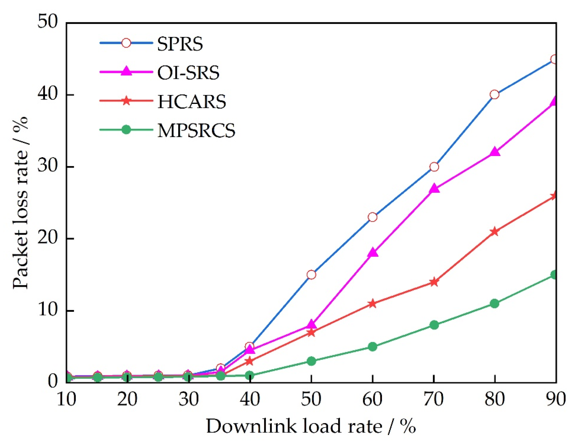
5.3. Comparison and Analysis of the Routing Control Strategy

To perform the routing control comparison, different methods have been compared including the Shortest path routing strategy (SPRS) [25], the hybrid Congestion alleviation routing strategy (HCARS) [26], the online increasing fit first segment routing strategy (OI-SRS) [27], and the proposed minimum path selectivity routing control strategy (MPSRCS). Several parameters have been employed to evaluate the comparison performance including the packet loss rate, the network transmission delay and the average bandwidth occupancy rate of downlink routing. The network parameters are set up as follows: spreading factor = 7, number of gateways is 3, number of nodes is 20; CR_min = 25, which is the minimum number of links in the network; CR_max = 35, which is the maximum number of links in the network; RB_max = 40 Mbit/s, which is the maximum link bandwidth in the network; RB_min = 0.0625 Mbit/s, which is the minimum link bandwidth in the network; RT_max = 20 s, which is the maximum link delay in the network; and RT_min = 10 s, which is the minimum link delay in the network. The average request bandwidth is gradually increased, and the network performance parameters under different routing control strategies are analyzed. Then, the downlink load rate h_m is defined as follows:

$$h_m=(\frac{h_i}{h_{\max }})\times 100\%$$

(19)

where, h_i is the current downlink traffic, and h_max is the downlink bandwidth value. Figure 15 shows the comparison of the packet loss rate under different downlink load rated.

Figure 15. Comparison of the packet loss rate under different downlink load rates.

In Figure 15, it is seen that when the downlink load rate is gradually increased, the packet loss rate of the MPSRCS is much less than those of the SPRS, HCARS and OI-SRS. The loss rate of SPRS is the largest since there is no link status detection in the process. When the load rate is relatively small, the loss rates of both the OI-SRS and HCARS are almost the same. When the load rate is further increased (exceeding 50%), the HCARS behaves relatively better than OI-SRS. It is known that the segment flow scheduling is used in the OI-SRS, and therefore the communication reliability can be ensured when the load rate is low. When the load rate exceeds 50%, it is seen that the communication reliability can be no longer guaranteed. In the HCARS, the dynamic process of route assigning is considered and therefore it is able to supply better reliability than those of the SPRS and OI-SRS. However, the bandwidth occupancy rate prediction is missing in this strategy and the dynamic response of the routing assigning in the dynamic process could be limited and this is the reason that the loss rate becomes larger when the load rate exceeds 70%. The proposed MPSRCS strategy fully considers the prediction of the link bandwidth occupancy rate. It is seen that the communication reliability of data transmission is better than the other three strategies.

Transmission delay is also an important parameter to evaluate the routing control performance. By considering the difference in the data transmission delay requirements of different downlink services in the LoRaWAN network, it is assumed that the average transmission delay of the downlink communication of the LoRaWAN network with a stable transmission in period (t, t + T) is $T\left(X\right)$. The maximum value of the transmission delay is set as $T_{\max }\left(X\right)$. The downlink data type of LoRaWAN is set as 3, and the average transmission delay $T_{delay}$ can be described as follows:

$$T_{delay}=\left[{\displaystyle \sum _{X=1}^{3}T(X)/T_{\max }(X)}\right]/3$$

(20)

Figure 16 shows the comparison of the average transmission delay of the downlink communication. It can be seen that different routing control policies demonstrate different delay regulation performances. When the load rate is small, due to the algorithmic complexity, the average transmission delay of the MPSRCS is slightly higher than those of the OI-SRS, SPRS and HCARS. When the load increases, the proposed MPSRCS demonstrates the best delay regulation performance. Time delay for the SPRS is large and this is because the segmented route assignment adds extra time in the process. Delay regulation of the HCARS is acceptable. However, this strategy is likely to fall into the local optimal route since the bandwidth occupancy rate of some certain neighboring nodes have great influence on the real-time status of the downlink. Compared with other strategies, the proposed MPSRCS strategy is more stable and less volatile.

Figure 16. Comparison of the average transmission delay of LoRaWAN downlink communication.

Figure 17 shows the comparison of the average bandwidth usage for downlink communication. As can be seen from Figure 17, due to the random nature of route assignment, the shortest route may have multiple data streams at the same time, which may cause uneven allocation of link resources and link congestion. This is the reason that the occupancy rate of the SPRS is saturated firstly in the four strategies. The occupancy rate performance of the HCARS is better than the OI-SRS. When the link is congested, the HCARS policy can adjust the downlink bandwidth occupancy rate in time, and gradually adjust the average requested bandwidth to a larger value and therefore relieve the link congestion. However, when the requested bandwidth is further increased, congestion still can be observed in the HCARS. The proposed MPSRCS strategy is able to predict the bandwidth occupancy rate in the link. The evaluation mechanism is calculated in advance for the potential future congestion situation, and the idle resources in the link are redistributed reasonably. Therefore, the average bandwidth occupancy rate is significantly higher than those of the SPRS, OI-SRS and HCARS, which makes the network resource allocation mechanism of downlink communication more effective.

Figure 17. Comparison of average bandwidth occupancy.

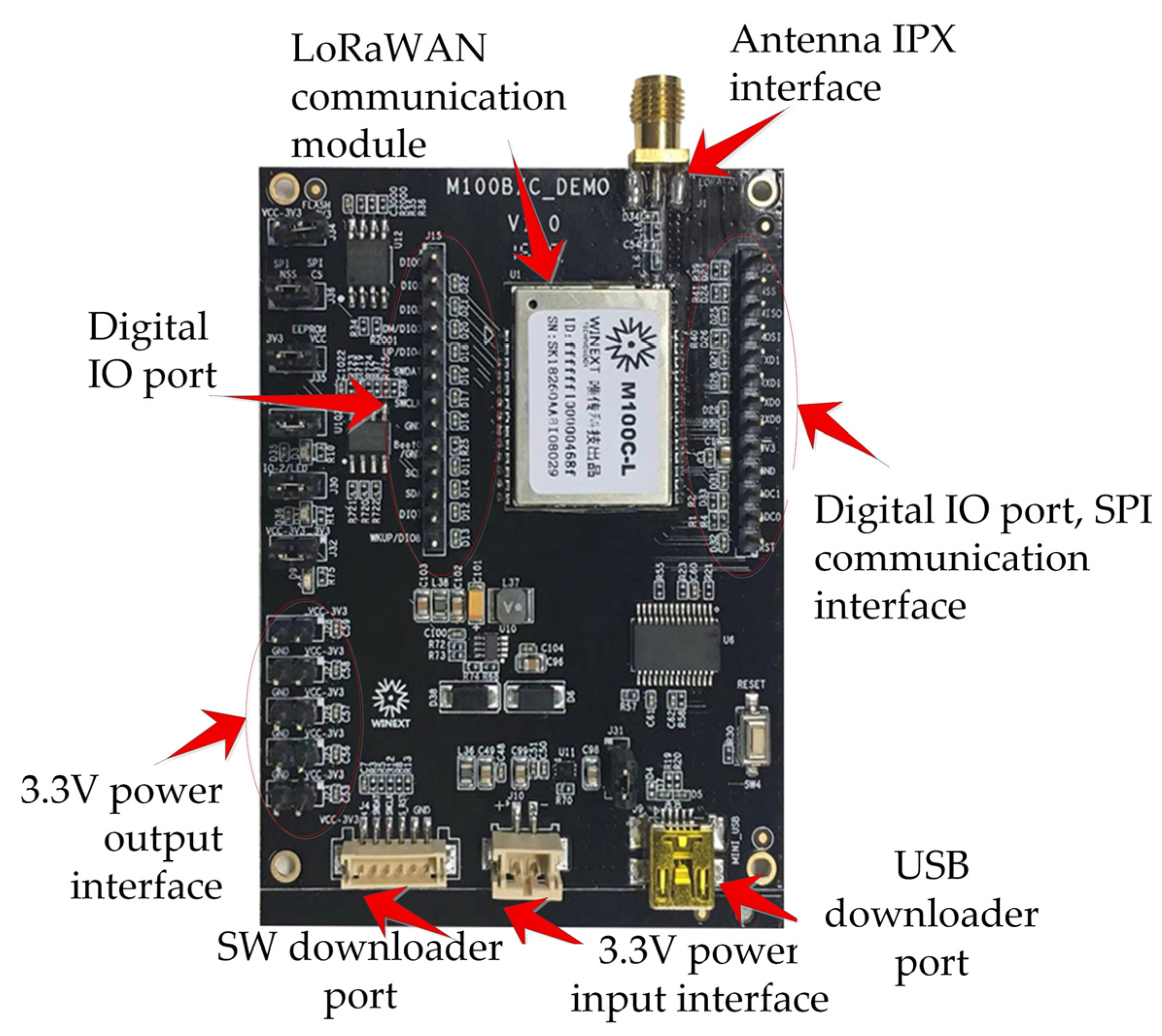
5.4. Experimental Platform

To run the experimental verifications, the middleware cloud is deployed on the Linux operating system by Docker, and the IoT LoRaWAN system architecture is used to realize service discovery and management. Here, we use the local host as the requester to simulate user requests. Figure 18 shows the successful startup of the middleware software. After the network service is started, the actual server address is configured in the LoRaWAN gateway according to the cloud middleware. The gateway hardware is shown in Figure 19 and the hardware description is listed in Table 6. The terminal module is connected to the LoRaWAN network via the gateway. The cloud platform is used to periodically send out data to the terminal nodes. the LBOP-ARIMA model proposed in this paper is applied to predict the downlink bandwidth occupancy and thereby perform the MPSRCS for the optimal downlink route selection. The optimal route to reach the best performed gateway is selected so that the downlink data packet joins the gateway data sending queue. When the terminal node receives the data sent out by the gateway, the MCU side responds in time and parses the data packet. The node data is uploaded to the platform side according to the downlink data request. Figure 20 is a prototype of the terminal node device.

Figure 18. The successful startup of the middleware software.

Figure 19. The LoRaWAN gateway hardware.

Table 6. The LoRaWAN gateway hardware description table.

Label	Name	Label	Name
1	Power indicator	11	SX1301 board power indicator
2	WI-FI indicator	12	4G module main antenna IPEX interface
3	USB indicator	13	48 V power interface
4	WAN indicator	14	Power supply 12 V ground interface
5	LAN indicator	15	12 V power input interface
6	3G/4G indicator	16	WAN interface
7	WiFi antenna SMA interface	17	LAN interface
8	LoRa antenna SMA interface	18	Hardware reset button
9	GPS antenna SMA interface	19	Factory reset button
10	LTE antenna SMA interface

Figure 20. Terminal node module prototype.

Here, the strategy performance of the HCARS and MPSRCS are compared. The link bandwidth occupancy is compared under different load rates and the results are shown in Figure 21. It is seen that when the link load rate is small, there is no significant difference. With the continuous increase of the downlink load rate, the link bandwidth occupancy rate of the MPSRCS demonstrates better performance. It is calculated that the overall average link bandwidth occupancy rate of the MPSRCS strategy is increased by 12% compared with the HCARS, which effectively improves the overall performance and reliability of the LoRaWAN network.

Figure 21. Terminal node module prototype.

6. Conclusions

The SDN framework is introduced into the traditional LoRaWAN downlink network, and a minimum routing degree routing control strategy based on the improved ARIMA algorithm is proposed in this paper. The SDN is adopted to monitor network traffic, and the link bandwidth occupancy rate is calculated based on the monitored downlink traffic. The S–G filtering algorithm is added to the ARIMA modeling process, and the time series data of the link bandwidth occupancy rate is processed for stationarity by combining the sliding window method and the high-order fitting polynomial. The triangle module operator is used for calculating the selectivity of each link to finally select the optimal route for LoRaWAN downlink communication. It is found that:

(1) Compared with the original scheme, the root mean square error of the improved ARIMA model is reduced by 87%, and the model prediction accuracy is significantly improved.

(2) Experimental results show that when applying with the proposed routing control strategy, the average bandwidth occupancy rate of the link is increased by 12%, which effectively improves the downlink communication performance and the reliability of the LoRaWAN network.

References

1. Centenaro, M.; Vangelista, L.; Zanella, A.; Zorzi, M. Long-Range Communications in Unlicensed Bands: The Rising Stars in the IoT and Smart City Scenarios. IEEE Wirel. Commun. 2016, 23, 60–67. [Google Scholar] [CrossRef] [Green Version]
2. Ramadhan, H.; Yustiawan, Y.; Kwon, J. Applying Movement Constraints to BLE RSSI-Based Indoor Positioning for Extracting Valid Semantic Trajectories. Sensors 2020, 20, 527. [Google Scholar] [CrossRef] [PubMed] [Green Version]
3. Singh, D.P.; Pant, B. An Approach to Solve the Target Coverage Problem by Efficient Deployment and Scheduling of Sensor Nodes in WSN. Int. J. Sys. Assur. Eng. Manag. 2017, 8, 493–514. [Google Scholar] [CrossRef]
4. Rizzi, M.; Ferrari, P.; Flammini, A.; Sisinni, E.; Gidlund, M. Using LoRa for Industrial Wireless Networks. In Proceedings of the 2017 IEEE 13th International Workshop on Factory Communication Systems (WFCS), Trondheim, Norway, 31 May–2 June 2017; pp. 1–4. [Google Scholar]
5. Judge, M.A.; Khan, A.; Manzoor, A.; Khattak, H.A. Overview of Smart Grid Implementation: Frameworks, Impact, Performance and Challenges. J. Energy Storage 2022, 49, 104056. [Google Scholar] [CrossRef]
6. Boccardi, F.; Heath, R.W.; Lozano, A.; Marzetta, T.L.; Popovski, P. Five Disruptive Technology Directions for 5G. IEEE Commun. Mag. 2014, 52, 74–80. [Google Scholar] [CrossRef] [Green Version]
7. Lien, S.-Y.; Chen, K.-C.; Lin, Y. Toward Ubiquitous Massive Accesses in 3GPP Machine-to-Machine Communications. IEEE Commun. Mag. 2011, 49, 66–74. [Google Scholar] [CrossRef]
8. Chen, S.; Hu, J.; Shi, Y.; Zhao, L. LTE-V: A TD-LTE-Based V2X Solution for Future Vehicular Network. IEEE Internet Things J. 2016, 3, 997–1005. [Google Scholar] [CrossRef]
9. Van den Abeele, F.; Haxhibeqiri, J.; Moerman, I.; Hoebeke, J. Scalability Analysis of Large-Scale LoRaWAN Networks in Ns-3. IEEE Internet Things J. 2017, 4, 2186–2198. [Google Scholar] [CrossRef] [Green Version]
10. Sakkari, D.S.; Basavaraju, T.G. GCCT: A Graph-Based Coverage and Connectivity Technique for Enhanced Quality of Service in WSN. Wirel. Pers. Commun. 2015, 85, 1295–1315. [Google Scholar] [CrossRef]
11. Centenaro, M.; Vangelista, L.; Kohno, R. On the Impact of Downlink Feedback on LoRa Performance. In Proceedings of the 2017 IEEE 28th Annual International Symposium on Personal, Indoor, and Mobile Radio Communications (PIMRC), Montreal, QC, Canada, 8–13 October 2017; pp. 1–6. [Google Scholar]
12. Minhas, H.I.; Ahmad, R.; Ahmed, W.; Waheed, M.; Alam, M.M.; Gul, S.T. A Reinforcement Learning Routing Protocol for UAV Aided Public Safety Networks. Sensors 2021, 21, 4121. [Google Scholar] [CrossRef]
13. Di Vincenzo, V.; Heusse, M.; Tourancheau, B. Improving Downlink Scalability in LoRaWAN. In Proceedings of the ICC 2019—2019 IEEE International Conference on Communications (ICC), Shanghai, China, 20–24 May 2019; pp. 1–7. [Google Scholar]
14. Liang, G.; Yu, H.; Guo, X.; Qin, Y. Joint Access Selection and Bandwidth Allocation Algorithm Supporting User Requirements and Preferences in Heterogeneous Wireless Networks. IEEE Access 2019, 7, 23914–23929. [Google Scholar] [CrossRef]
15. AbdelBaky, M.; Diaz-Montes, J.; Parashar, M. Software-Defined Environments for Science and Engineering. Int. J. High Perform. Comput. Appl. 2018, 32, 104–122. [Google Scholar] [CrossRef] [Green Version]
16. Tomovic, S.; Radusinovic, I. RO-RO: Routing Optimality—Reconfiguration Overhead Balance in Software-Defined ISP Networks. IEEE J. Sel. Areas Commun. 2019, 37, 997–1011. [Google Scholar] [CrossRef]
17. Aujla, G.S.; Garg, S.; Batra, S.; Kumar, N.; You, I.; Sharma, V. DROpS: A Demand Response Optimization Scheme in SDN-Enabled Smart Energy Ecosystem. Inf. Sci. 2019, 476, 453–473. [Google Scholar] [CrossRef]
18. Bastam, M.; Rahimi Zadeh, K.; Yousefpour, R. Design and Performance Evaluation of a New Traffic Engineering Technique for Software-Defined Network Datacenters. J. Netw. Syst. Manag. 2021, 29, 38. [Google Scholar] [CrossRef]
19. Tomovic, S.; Radusinovic, I. Toward a Scalable, Robust, and QoS-Aware Virtual-Link Provisioning in SDN-Based ISP Networks. IEEE Trans. Netw. Serv. Manag. 2019, 16, 1032–1045. [Google Scholar] [CrossRef]
20. Li, H.; Ota, K.; Dong, M. Virtual Network Recognition and Optimization in SDN-Enabled Cloud Environment. IEEE Trans. Cloud Comput. 2021, 9, 834–843. [Google Scholar] [CrossRef]
21. Liu, C.; Liu, C.; Shang, Y.; Chen, S.; Cheng, B.; Chen, J. An Adaptive Prediction Approach Based on Workload Pattern Discrimination in the Cloud. J. Netw. Comput. Appl. 2017, 80, 35–44. [Google Scholar] [CrossRef]
22. Yi, J.; Adnane, A.; David, S.; Parrein, B. Multipath Optimized Link State Routing for Mobile Ad Hoc Networks. Ad. Hoc. Netw. 2011, 9, 28–47. [Google Scholar] [CrossRef] [Green Version]
23. Al-Kashoash, H.A.A.; Amer, H.M.; Mihaylova, L.; Kemp, A.H. Optimization-Based Hybrid Congestion Alleviation for 6LoWPAN Networks. IEEE Internet Things J. 2017, 4, 2070–2081. [Google Scholar] [CrossRef]
24. Cao, Y.; Wu, M. RPL Based on Triangle Module Operator for AMI Networks. China Commun. 2018, 15, 162–172. [Google Scholar] [CrossRef]
25. Altın, A.; Fortz, B.; Thorup, M.; Ümit, H. Intra-Domain Traffic Engineering with Shortest Path Routing Protocols. Ann. Oper. Res. 2013, 204, 65–95. [Google Scholar] [CrossRef]
26. Al-Kashoash, H.A.A.; Kharrufa, H.; Al-Nidawi, Y.; Kemp, A.H. Congestion Control in Wireless Sensor and 6LoWPAN Networks: Toward the Internet of Things. Wirel. Netw. 2019, 25, 4493–4522. [Google Scholar] [CrossRef]
27. Cianfrani, A.; Listanti, M.; Polverini, M. Incremental Deployment of Segment Routing into an ISP Network: A Traffic Engineering Perspective. IEEE Trans. Netw. 2017, 25, 3146–3160. [Google Scholar] [CrossRef]