Information Technologies for Real-Time Mapping of Human Well-Being Indicators in an Urban Historical Garden

Abstract

The post-pandemic era has raised awareness on the importance of physical and psychological well-being for decreasing the vulnerability of both individuals and populations. Citizens in urban areas are subject to numerous stress factors which can be mitigated by green spaces such as parks and gardens. Sensor and internet technologies support nature-based solutions in various ways. In this paper, we show the results of ongoing research on the use of spatially distributed IoT sensors that collect climate data in an ~8 ha urban garden. The novelty resides in the method for merging the IoT data with a detailed 3D model created by a laser scan survey from a drone flight. The end products are 1 m resolution thermal comfort maps of user-defined scenarios, e.g., at specific times or aggregated in daily/monthly/yearly statistics that represent a thermal comfort distribution. For full replicability, the code is open source and available as an R package on Github.

1. Introduction

Among the seventeen Sustainable Development Goals (SDGs) of the United Nations, there are “good health and well-being” (SDG three) and “sustainable cities and communities” (SDG eleven). To support these goals, new technologies related to data survey can provide important information for decision makers. According to the 2014 UN-ESA report, the percentage of people living in urban areas is expected to increase from 54% up to 66% by 2050. Urban gardens play a key role in improving the living quality of citizens. Not only do urban gardens mitigate the temperatures of heat islands, but they also provide green spaces to visitors who can experience being close to a natural environment [1]. In this work, we assess the feasibility of using internet of things (IoT) sensors and a detailed and accurate three-dimensional (3D) model of a historical urban garden to map comfort indicators related to climatic variables. We foresee that these technologies will, in the near future, be replicated for better planning of parks, gardens, and visits, as well as for a better understanding of human behavior in green areas [1].

1.1. Comfort Indicators

The environmental variables and morphological characteristics of the natural and artificial environments at the urban scale influence the comfort and behaviors of the citizens. Urban parks and gardens play a key role in creating a microclimate that can bring well-being to humans. Wellness resulting from exposure to the natural environment is both physical and psychological. The latter aspect is one of the impacted factors during and after the COVID-19 pandemic, with differences depending on age [2]. Climate and environmental factors influence the human body during visits to gardens. The literature refers to the heat-balance model of the human body [3] to measure this effect. Heat-balance considers the metabolic rate, the physical work output, the net radiation of the body, the storage of heat flow or cooling, and the convective heat flow but also the heat flow to evaporation through the skin, the sweat and humidity of the air, the effective temperature (ET) [4], and the Gage two-node model. These models have been applied in the heat-balance by the Munich energy-balance model for individuals (MEMI) [5], which is the base for the calculation of the physiological equivalent temperature (PET) and the standard effective temperature (SET). PET is defined as the air temperature at which, in a typical indoor setting (without wind and solar radiation), the heat budget of the human body is balanced with the same core and skin temperature as under the complex outdoor conditions to be assessed [6]. SET considers the temperature of a hypothetical isothermal environment at 50% or relative humidity in which a human subject while wearing clothing, standardized for the activity concerned, would have the same skin wetness and heat exchange at the skin surface as he would have in the actual test environment [7]. The difference between the PET and SET is that the reference environment considers the skin and core temperatures rather than the temperature and humidity at skin level. However, the same environmental parameters are used in both formulas. The predicted mean vote (PMV) index is a thermal sensation measure with values that range from −3 to +3 which describe the feeling from too cold to too hot respectively, with zero being a neutral vote and thus maximum comfort [8].

Comfort indices consider physiological and environmental parameters. Four are environmental parameters: (i) air temperature, (ii) mean radiant temperature, (iii) wind velocity, (iv) humidity. Two are physiological factors: (i) clothing level and (ii) metabolism at 20 °C. Clothing level can have a value from zero to one, and metabolism can be expressed as energy flux, e.g., 81 W/m² for slow walking. Hence, comfort indices are normalized for clothing and metabolic activity, focusing on the four environmental parameters listed above.

Other studies have highlighted the thermo-physiological effect of short-wave and long-wave radiation fluxes in human beings under both indoor and outdoor conditions [9]. In this sense, the RayMan model estimates the direct and reflected solar radiation in the three-dimensional space that surrounds the human body under the different visible sections of the sky and canopy cover using pyranometers and hemispherical photos. However, RayMan is a stationary model influenced by the complexity of the urban environment, such as the presence of structures [10]. On the other hand, potential issues in the estimation of comfort indices are related to data collection, especially in non-stationary conditions or for long-lasting experiments. Outdoor environments are complex scenarios for comfort calculation, where tall vegetation and a mixture of buildings, vegetation, direct and diffuse solar radiation conditions that depend on atmospheric conditions, and shade from vegetation or buildings have to be accounted for.

1.2. Modelling Direct/Diffuse Solar Radiation

In an environment with tall vegetation, the influence of the spatial distribution of canopies plays a key role in calculating comfort indices at a specific position in space. A location will receive a certain fraction of direct vs. diffuse radiation from sunlight depending on the time of day, day of the year, and nearby objects. The quantification of the effect of canopy obstruction/gaps with respect to solar illumination is an important parameter that affects comfort indices as well as ecological diversity, as direct sunlight can affect the microclimate with impacts on the habitat distribution of plants and animals [11]. The estimation of the canopy cover and the amount of the leaf area is a critical process performed by terrestrial surveys, measuring the width and length of the gaps using hemispherical images or by applying remote sensing analysis [12]. None of the methods can be considered better than any others, since they are affected by bias and estimation errors [13,14], but the hemispherical photo method is the most widely used technique. For extensive areas, remote sensing analysis is preferred in contrast to a terrestrial investigation, which is time-consuming and expensive [15].

As mentioned above, indicators of people’s physiological comfort, but also psychological well-being, are calculated using the environmental variables. Those indices can give guidance for urban planning at different scales for studying the interaction of the microclimate in urban gardens and parks. Physiological comfort and psychological well-being, resulting from exposure to vegetation, are related to the canopy distribution, presence of buildings and water bodies, and variates seasonally [16]. In addition, these areas are aggregation spots that attract different types of users, from the young to the elderly, and each of these groups has different requirements regarding well-being. Data collected with sensors placed at 1.5 m above the ground between 7:00 AM and 5:00 PM have shown a high correlation between PET and solar radiation, where the feeling of comfort increases in naturally and artificially shaded areas and near water [17]. A study conducted on eight gardens in Chengdu City showed the optimal ratio between evergreen and deciduous plants to be 1:3, where the elderly need a more warm, humid, and sunlight-exposed microclimate to improve their degree of comfort [18].

In this study, we calculate and map comfort indices of the garden of Villa Revedin-Bolasco using a real-time data flow of environmental variables. We map the spatial distribution of direct solar radiation values using a 3D model from an airborne LiDAR acquisition of the entire garden. We describe the implementation of a LoRa IoT network in the garden of Villa Revedin Bolasco for collecting data from several environmental sensors. The LoRa antennas collect, in real-time, the data streams of several environmental sensors installed in the garden in a fixed position that can also be deployed on a mobile rover. The environmental variables, namely the air temperature, relative humidity, solar radiation, wind speed, wind direction, and air quality, are stored in a database management system (DBMS). The advantage of this method is the creation of an accessible, spatially distributed, temporally dense data repository of several environmental variables. Moreover, data visualization and analysis are implemented on a web application, so that comfort maps can be calculated in real-time and integrated into a geographic information stem (GIS), and/or simulations of comfort can be carried out at the scale of the urban garden.

2. Materials and Methods

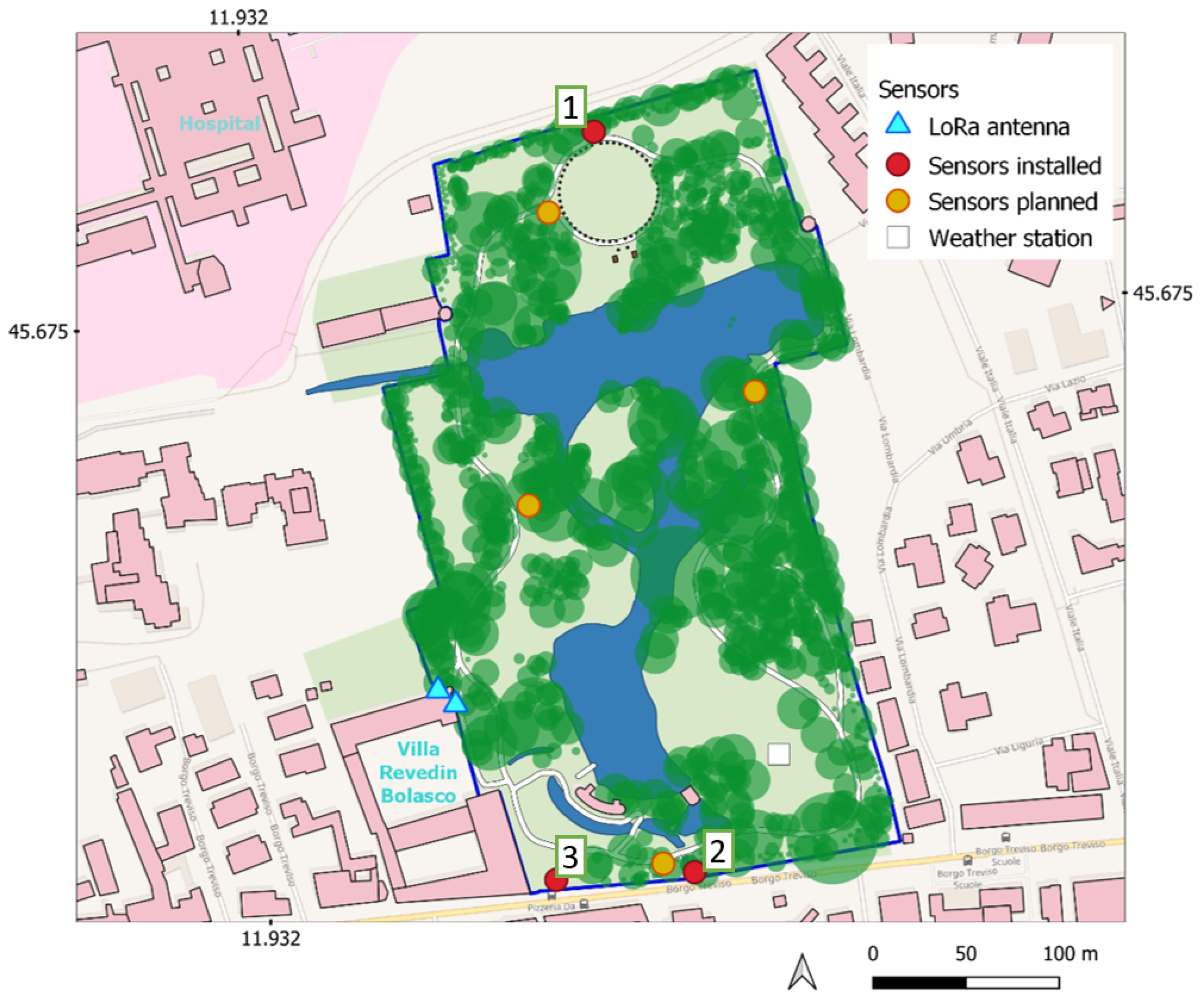
2.1. Study Area

The study area is the garden of the Villa Revedin Bolasco located in the city of Castelfranco Veneto, Northeast Italy. Villa Revedin Bolasco was built as a private residence in the middle 19th century by Count Francesco Revedin. An English garden, which extends over an area of 7.63 hectares, enriches the magnificence of the Villa. The garden has a tree count of over 1000 and it includes a lake, bridges, lawns, hillocks, and an equestrian arena, which is a man-made depression. Figure 1 provides a schematic overview with geographic coordinates in WGS-84 data. The villa is part of the European Union’s Horizon 2020 Research and Innovation programme VARCITIES, with the pilot city of Castelfranco Veneto. The project’s vision is to implement nature-based actions in cities. Investigating sustainable models for increasing the health and well-being of citizens exposed to different climatic conditions and challenges was applied to this study area by using information and surveying technologies to map comfort indices for visitors of the historical garden of Villa Revedin Bolasco. The methods section is divided into four parts that regard the following aspects: (i) the sensors that are used for collection of climatic data, (ii) the sensors’ data flow and storage solutions, (iii) the 3D model and its use for mapping direct solar radiation, and (iv) the merging of the 3D model and the climate data to map the comfort indices.

2.2. Sensors and Geopositioning

The IoT infrastructure for data collection in the garden of Villa Revedin Bolasco was implemented via a gateway with two antennas. The gateway for LoRaWAN was a WisGate Edge Max RAK7249 and the 2 antennas are 8dBi fiberglass antennas. The antennas are omnidirectional, but due to limitations regarding the cultural heritage site, they had to be positioned just outside the top floor of a building and not on the rooftop. To obtain the most coverage, the two antennas were positioned at opposite sides of a corner, thus covering all parts of the garden (see Figure 1).

To cover the area of the garden, a total of 27 IoT devices were initialized and geopositioned. A list of devices is available in

Table 1. List of sensors and models, with the number (N) installed in the garden.

Make, Model, (Abbreviation)	Sensors	N.
Synetica enLink Air-X (Syn-Air)	temperature, relative humidity, barometric pressure, ozone, oxygen, carbon dioxide, nitrogen dioxide, volatile organic compounds (VOC), and particles as PM 1, 2.5, 4, 10 (quality measurement)	3
DecentLab DL_ATM22 (DL-Atm)	temperature and wind speed and direction vectors	3
DecentLab DL_PYR (DL-Pyr)	pyranometers for measuring solar radiation	7
Iotsens Sound Level (Iot-Snd)	noise level	3
Davis Pro weather station (DP-Wst)	temperature, barometric pressure, humidity, rainfall, solar and UV radiation, wind speed, and wind direction	1
Sensedge Senstick (Sen-Stk)	temperature, humidity, and acceleration	10

. with their positions visible in Figure 1. Note the fact that there are not 27 locations because more than one sensor model can be placed in the same spot, e.g., the pyranometers with climate sensors and atmospheric sensors such as in Figure 2.

The majority of the sensors were placed on a fixed pole at 1.5 m above the ground level at specific locations of interest. The points of interest were near park benches, which are rest areas where young and elderly visitors can sit, talk, and enjoy the garden. The power source was provided by alkaline batteries that guarantee a minimum operating time of 5 months up to 11 years depending on the sensor, except for the Synetica enLink Air-X and Iotsens Sound Level, which require alternating current power supplies.

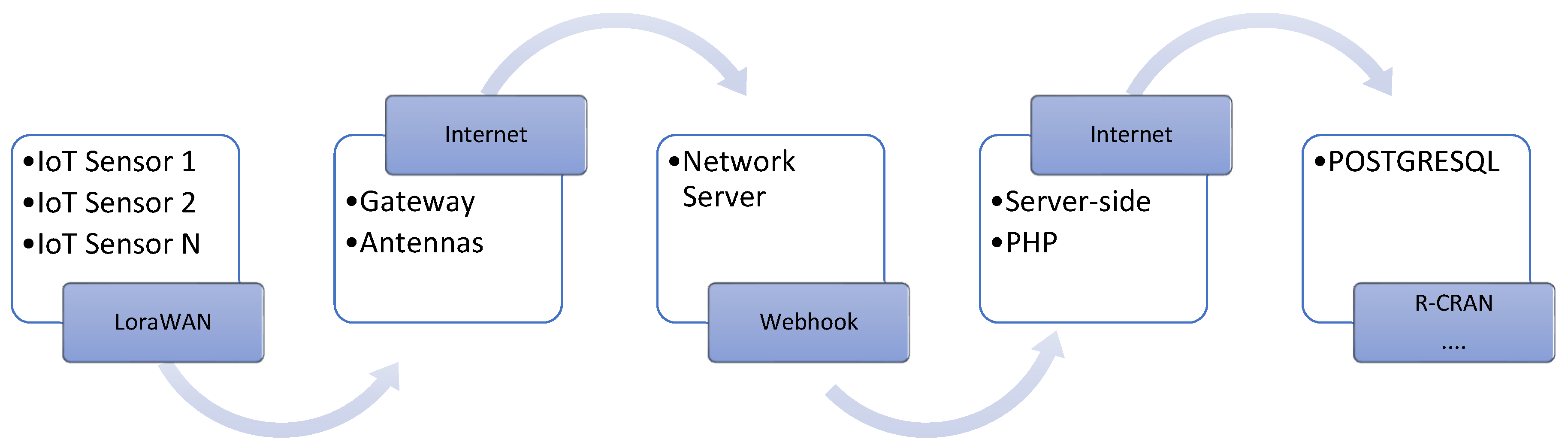
2.3. Data Flow and Storage

The data flow from the sensors to a storage solution is summarized in Figure 3. The sensor emits a payload with stored data to the gateway which is registered to a network server that manages sensors and gateways. The network server is The Things Stack, an open source LoRaWAN network server that can be hosted free of charge for small networks. All payloads are decoded to an ASCII readable format, i.e., JSON. The data are intercepted via a webhook. The webhook is a web-reachable page with a server-side script in PHP that redirects the data to a PostgreSQL database server. The data are stored in a JSON binary format (JSONB class in PostgreSQL) in a table with three columns: a timestamp column, a device id, and the JSON payload. The table does not have any indexing, triggers, or constraints in order to limit any overhead in data insertion. This table with raw data is then used to create derived tables using views and materialized views that provide the right formats and units for using them in further calculations. For example, in some sensors barometric pressure is provided in the unit of inches of Hg (mercury) and further processing requires millibars.

2.4. 3D Models

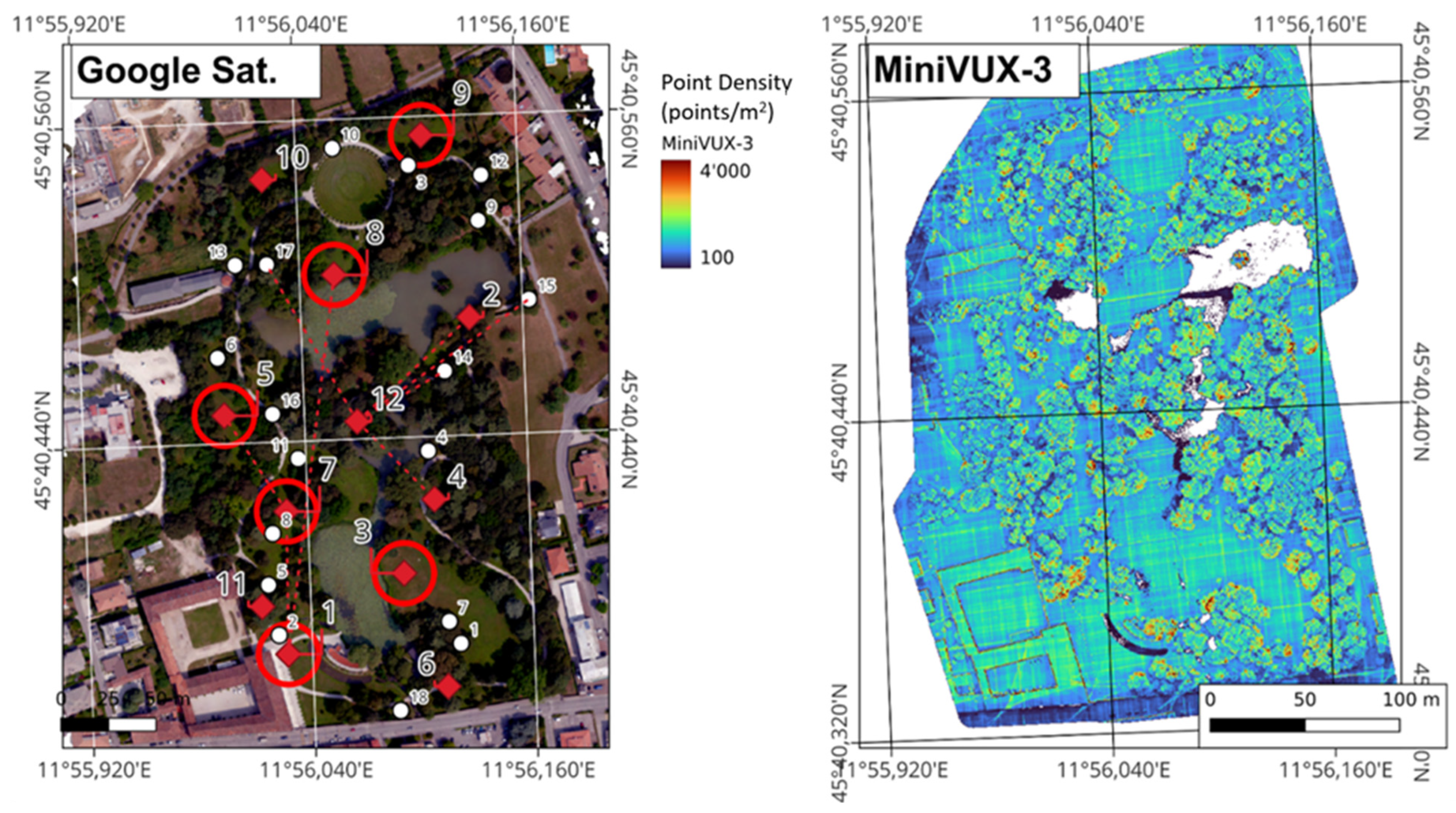
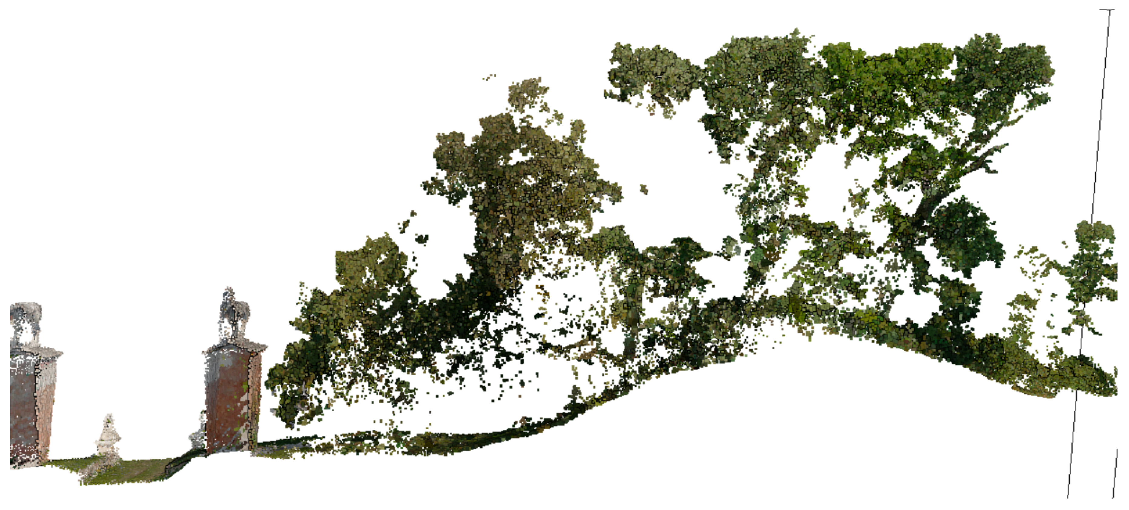
2.4.1. Laser Scanning Survey

The historical garden has a complex morphology consisting of different species of trees, small hills, a lake, and artificial depressions. Consequently, a digital terrain model (DTM) and a 3D point cloud (3DPC) representing the vertical structure of the elements above the terrain are essential in the analysis. The 3DPC was obtained through a flight with an unmanned aerial vehicle (UAV) in July 2021 using Rigel VUX-3 light detection and ranging (LiDAR) sensor. Ground control points (GCPs) and check points (CPs) were surveyed with an RTK GNSS receiver providing coordinates with an accuracy of ~0.025 m (RMSE). A comparison between different sensors from the same survey provides an overall expected absolute accuracy for each point of ~0.05 m (see the authors’ work in [19]). The LiDAR sensor has a framerate of 200,000 measurements per second that return 3D coordinates and intensity of reflective surfaces that cause diffuse reflectance of the laser pulse. This resulted in a 3DPC with an average point density of ~1000 points per square meter (Figure 4, right) and a detailed 3D representation of the vertical structure of vegetation (Figure 5).

2.4.2. Digital Terrain Model

The DTM was created by interpolating all points classified as “ground” points in the 3DPC. Ground points were extracted from the 3DPC using an adaptive iterative triangulation algorithm [20]. This method creates an initial tringle irregular network (TIN) mesh from a set of a few candidate points consisting of points with local minimum heights. The term “local” implies that the selected points are those with the lowest height values in an area that is at least as big as the smallest area that is supposed to have at least one ground point. The choice of the value of the minimum area to search for the lowest 3D point is defined by the user and it depends on the data and the location scenario. In urban areas, it consists of the footprint area of the largest building. In thick forests, this value can be larger. In our context, we chose a 10 m radius to define the minimum area, as this point density provided a high probability of ground returns under the thick canopies of the garden. From the rough TIN mesh, each remaining point from the 3DPC assigned to the TIN if it meets certain criteria, and thus the TIN is iteratively densified to a ground surface.

2.4.3. Shadow-Casting Model

Predicting the distribution of shadows in the garden is fundamental in order to calculate the mean radiant temperature of surfaces that are hit by direct solar radiation. In this case, we only considered the human body as the surface, and we ignored other surfaces because most of the other surfaces consist of vegetation, which does not significantly emit back heat that changes the perceived temperature of the person walking in the garden. In some areas of the garden, the canopy covers are packed together on a continuous surface where the shadows are projected around the canopies, but the surface from a nadiral view seems completely illuminated. However, looking at the canopy from a zenithal point of view as a hemispherical photo taken from the ground, the illumination can be diffuse, and the direct light can pass or be blocked by the leaves and branches. Therefore, the pixels of the illumination map, which are under a dense canopy cover, have been considered illuminated or shadowed relating to their gap fraction values. A simulated shadow map every 15 min is available as an animation in the Supplementary Material (S1), which is part of the R CRAN package available for replicability of the method proposed in this article.

2.5. Comfort Indices Calculation

The calculation of comfort indicators considers the environmental and physiological variables reported in the introduction. The details of the PET equation are reported in the work of [21]. The procedure was implemented in R in the rPET package that is available for replicability of the method (https://github.com/fpirotti/rPET, accessed on 20 September 2022). Several climatic variables are measured and available from the IoT sensors, i.e., air temperature, wind velocity, barometric pressure, and humidity. An important variable, the mean radiant temperature (Tmr), is the factor that changes in different shade situations and affects the values and relative comfort indicator significantly when other factors are constant. As defined by [22,23], the mean radiant temperature is what changes when the human body is exposed to full sunlight or the sunlight is partially obstructed (shadow). One formula used for calculating Tmr is the following:

$$Tmr={\left[{\left(Tg+273.15\right)}^4+2.5\times {10}^{-8} · W{V}^{0.6}·\left(Tg-Ta\right)\right]}^{0.25}-273.15$$

(1)

where Tg is globe temperature in degrees Celsius, WV is wind velocity in m⋅s⁻¹, and Ta is air temperature in degrees Celsius. Globe temperature can be measured using specific instrumentation, but in this case, it has to be estimated. We use the following equations from [24,25] to estimate Tg:

First, we calculate atmospheric vapour pressure and then the thermal emissivity.

$$Ea=\left[\exp \left(\frac{17.67·\left(Td-Ta\right)}{Td+243.5}\right)·\left(1.0007+0.00000346·P\right)·6.112·\exp \left(\frac{17.502·Ta}{Ta+240.97}\right)\right]$$

(2)

$${\epsilon }_a=0.575·E{a}^{1/7}$$

(3)

where Ea is atmospheric vapour pressure, Ta is air temperature, Td is dew point temperature (°C), and ε_a is the thermal emissivity. We then calculate two arguments B and C as follows:

$$B=S·\left(\frac{f_{db}}{4·\sigma ·\cos \left(\mathrm{z}\right)}+\frac{1.2}{\sigma }·f_{dif}\right)+{\epsilon }_a·T{a}^4$$

(4)

where σ is the Stephen–Boltzmann constant and is equal to 5.67 × 10⁻⁸ (W⋅m⁻²⋅K⁻⁴) and S is solar irradiance (W⋅m⁻²), and f_db and f_diff are the fraction of direct-beam and diffuse sun radiation respectively.

$$C=\frac{0.315·u^{0.58}}{5.3865·{10}^{-8}}$$

(5)

where u is wind speed in meters per hour (WV m⋅s⁻¹ * 3600 s⋅h⁻¹). Finally, by combining C, B, and Ta the globe temperature can be calculated:

$$g=\frac{B+C·Ta+\mathrm{7,680,000}}{C+\mathrm{256,000}}$$

(6)

Once Tg is estimated, Equation (1) is used to extract mean radiant temperature that is used in the calculation of the comfort indices. It is worth noting that mapping these values implies that there are different values of mean radiant temperature depending on the position in space. The different values of mean radiant temperature are due to different proportions of direct beam illumination, which is the factor that changes significantly depending on how much shadow is cast in the area. Comfort indices also require other information, such as if the person is male or female, the clothing level, and the metabolic rate. Below are some values of possible metabolic rates (met) where 1 met = 58.2 W/m².

• Sleeping: 0.7 met, (41 W/m²)
• Reclining: 0.8 met, (47 W/m²)
• Seated, quiet, reading, writing: 1.0 (58.2 W/m²)
• Typing: 1.1 met, (64 W/m²)
• Standing, relaxed, seated: 1.2 (70 W/m²)
• Walking slowly: 1.4 met, (81 W/m²)
• Driving a car: 1.5 met, (87 W/m²)
• Walking at a medium speed: 1.7 met, (99 W/m²)
• Walking at 2 mph (3.2 km/h): 2.0 met, (116 W/m²)
• Light machine work: 2.2 met, (128 W/m²)
• Walking at 3 mph (4.8 km/h): 2.6 met, (151 W/m²)
• House cleaning: 2.7 met, (157 W/m²)
• Driving, heavy vehicle: 3.2 met, (186 W/m²)
• Dancing: 3.4 met, (198 W/m²)
• Walking at 4 mph (6.4 km/h): 3.8 met, (221 W/m²)
• Heavy machine work: 4.0 met, (233 W/m²)

2.6. Shadow-Casting Estimation

Mapping light and shadow as described in Section 2.4.3 is fundamental for Equation (4). Here is where the 3D model is used. First, we create a grid with nodes spaced at 1 m distance. Each node represents the position of a person standing on the surface of the study area. To find this information, the DTM nodes are used, which represent the height above sea level of the bare ground without trees or buildings. The height values are raised 1.5 m above the ground to simulate the chest height of an average person standing on the terrain of the historical garden, i.e., visiting the premises. This value can be changed by the user, using the webapp to simulate light and shadow fractions. Using a ray-casting approach, we calculate the fraction of direct solar illumination (f_db) arriving at each cell, as required by Equation (4).

2.7. R Package and Webapp

All methods described above are wrapped in a R CRAN package called rPET. R is a well-known programming environment that started out for statistical analysis and has now expanded to provide processing tools for a very wide variety of applications, many of which take the spatial domain into account [26]. A new package developed in R, such as in this case, can include dependencies from existing packages, i.e., it can make use of functions and objects that are already implemented in another package in order not to “reinvent the wheel”. In our implementation, the following packages are used either directly as dependences or indirectly as forked code: (i) lidR [27] for 3D point cloud data processing, i.e., it was used to convert a file in LAS/LAZ format [28] to a matrix with 3D coordinates that represent the point cloud of the study area (see Figure 5) and is used as example data; (ii) the terra [29] package for processing all 2D raster data, such as the DTM and the creation of the final comfort maps; (iii) rayshader [30], from which the basic rayshade code was forked from and modified to enable actual 3D rayshading. The latter code is what maps the sun radiation considering the shadow effect from elements above the ground. The original rayshader code only considers a 3D surface and not a 3D point cloud. The main workload is related to mapping shadows over a 2D regular matrix that represents the positions of people at each node, as reported in Section 2.4.3.

To wrap all the processing in an interactive webapp, a function called “solarApp” is available to launch a web interface that allows the user to map the three comfort indices over the study area and change climate and physiological variables interactively. By forking the rPET package, a user can also tweak the code to define a different study area by just changing two input elements: (i) the DTM and (ii) the 3D point cloud source data. The solar angle is determined by the user or by the time of day and centroid position of the area in geographic coordinates.

The code is available at https://github.com/fpirotti/rPET (accessed on 20 September 2022) with some examples from [25]. This package is for research and is not expected to be included in the official R repository, but it can be installed directly in any recent R environment by following the directions contained in the readme file of the Github page.

3. Results

At this point in the research, the results are partly visual and obtained by means of cross-validation between three main sensors: the weather station and two locations in which multiple sensors providing environmental variables are installed (see Table 1 and Figure 1. sensor 1 and 2). In particular, the pyranometers provide the solar radiance and the temperature recorded by devices.

3.1. Webapp

Figure 6 shows an overview of the webapp that is deployable from the R package that can be installed following the directions in https://github.com/fpirotti/rPET (accessed on 20 September 2022). The rPET::solarApp() function runs a webapp where the user can insert environmental and physiological variables and calculate comfort indices on the fly. The DTM and 3D point cloud used in this paper are included in the package but not directly. They are downloaded automatically and added to the package environment the first time that the app is launched. This requires about 50 s and can also be performed preventively using a script called “preparedata.R”. This script can be tweaked for users to deploy their own DTM and point cloud data. The app will automatically center the geographic information system (GIS) in the right panel in the user area if the data are georeferenced correctly.

Figure 7 provides several outputs that can be obtained by calculating the comfort index at different times and days as well as calculating daily aggregation statistics such as the average, maximum, and standard deviation values of the comfort index. The statistics shown in the figure are related to which parts of the garden have an overall better value on average. Considering that July is a very hot month, the average comfort vote is higher than 0 (ideal) and towards a feeling of hotness, as seen in Figure 7f. The comfort index is only on average close to zero underneath the trees. A video of shadow degrees and comfort index variation over a single day every 15 min is available in the Supplementary Materials as S1 and S2, respectively. The ability to model maps of comfort indices with user-defined or sensor-derived inputs allows to provide cumulated statistics that can be used to assess overall comfort of an area. Considering that one of the independent climatic variables is the radiant temperature and that this depends on the 3D structure of the site, users can theoretically provide different virtual 3D models (e.g., different infrastructure plans) and map overall comfort of the different scenarios and assess the impact of each one. As can be seen in Figure 7e, some spots are with very little variation of comfort index, and this also has an impact on certain vegetation and animal species and is of interest for collating to biodiversity.

3.2. Sensors Comparison

To check the effect of shadow on climatic data collection, several sensors were compared: the weather station and three locations (Figure 1) with multiple sensors (Figure 2). It must be noted that the weather station records air temperature, whereas the two air-quality measurement devices record the temperature of the device itself, as, at this time, the sensor is not shielded. Therefore, it can be said that the air-quality sensors show the global temperature values (Equation (4)). The air-quality measurement devices are in shadow to differing levels, and this can be observed in Figure 8: at 8:00 a.m., the temperature of the 4815 device increases more than the reference temperature of the weather station. The same happens later, around 2:00 p.m. for the other device, 4816. These sensors are positioned in location 1 and 2 in Figure 1, respectively.

We extracted the predicted mean vote comfort index every 15 min for the 27th of July 2022 (Figure 9) to compare the relative relation of comfort values with recorded temperature values. The specific day was chosen from days belonging to the hot season (summer) and non-rainy days. A day with high temperatures and strong illumination provides a more variable daily comfort index and can thus help discriminate sensor and model behavior. It is expected that the shadow-casting prediction from the 3D model will mirror the temporal distribution of Figure 8. As matter of fact, we can see in Figure 9 that the two sensors predict the same comfort index around 14:00 (2:00 PM) which matches the distribution that we see in Figure 8.

A final cross-validation was performed directly using the solar radiation from pyranometers and the shade fraction from ray-casting illumination, at the coordinates of the pyranometers, using the 3D model. Figure 10 below shows how the values measured by the pyranometers every 15 min and the illumination fraction modelled at identical timestamps are highly correlated. A quantification by a simple linear model provides a coefficient of determination (R-squared) of 0.83 and 0.86 respectively for sensor 4815 and 4816.

4. Discussion

The webapp is an interactive tool that is very useful to promote awareness of how vegetation can be a valid support for improving comfort for visitors of the garden. It can act both as a simulation tool and for real-time mapping of comfort indices in the garden. Using weather forecasting tools, which are quite accurate at predicting weekly values of the climatic factors together with the model, can map comfort indices and thus support visits. In particular, elderly people or persons that have issues that limit or modify perception, e.g., Alzheimer’s disease, can make sure to visit the garden at dates and times when the comfort indices are ideal. To our knowledge, this is the first time that such a combination of IoT devices and 3D models are used together to provide an accurate geospatial map of comfort indices. Scientific literature at the regional and urban scale are common. The former is exemplified by the work of authors in [22], where satellite data is used to provide a global map of mean radiant temperature, which is an input in functions for comfort indices (see Equations (1)–(4)). The same authors provide a global mapping of comfort indices in [23]. At the urban scale, much work has been performed for energy efficiency modelling using 3D models [31]. At the urban scale, [32] used geographic information systems (GIS) to map bioclimatic comfort. The work of [33] maps comfort levels at an urban scale by considering streets in the city. Authors in [34] have used GIS at the scale of an urban park, also mapping visitor behavior with a significant dataset, with similarities to [1].

The main point of sensor data is to estimate the mean radiant temperature. As mentioned in [6], this can be estimated by cloud cover, time of the year, and type of surface cover. In this work, we estimate it by integrating sensors and a 3D point cloud model. Cloud cover is integrated into the model when directly using data sensors. Cloud cover is a factor that indirectly is considered by solar radiation sensors, e.g., pyranometers.

A network of low-cost sensors can directly measure sunlight/shadow and temperature, thus providing comfort indices that are not based on a model, but on direct measures. This solution would provide accurate indices, but only for the specific location where the sensors are placed. Light/shadow characteristics can vary greatly within a small distance, especially in complex scenarios with trees and buildings. This variability would require a large number of sensors to represent the study area. For example, in a summer day at the latitude of the study area, a person positioned in direct sunlight will feel too hot, whereas moving even one meter to where the vegetation can provide shadow and result in a much increased comfort. To catch this variability, sensors would have to be very dense, and this would increase maintenance costs. Additionally, to cover the entire area, data should also be spatially interpolated, thus adding uncertainty to the final values. Our proposed solution, being based on sensor data, but also on a physical model that defines the ratio of direct light beam and diffuse light only (shadow), provides a continuous cover of comfort values of the study area.

Cross-checking the hourly temperature distribution statistics from the two pyranometers and the weather station (Figure 9 and Figure 10) shows that the comfort indices reflect the temperature readings. This is an important validation as it means that the mapping of the comfort index accounts correctly for the spatial distribution of radiation. The spatial distribution of radiation influences the mean radiant temperature (Tmr) by modulating the arguments in Equation (4) i.e., the fraction of direct-beam radiation vs. diffuse radiation.

Another package in R, the comf package [35], also provides comfort indices, but not the PET index. It must be noted that it provides information related to room comfort and not for open environments. It does not include variables related to sun illumination. These variables can be determined by the shadow-casting map and Equation (4). In our application, this package was used for SET and PMV index by providing a mean radiant temperature factor calculated with the outdoor prediction of solar radiation. A similar approach has been used by other authors to map a single point-in-space comfort index [9,17].

It is worth noting that most comfort indices include solving a non-linear system of equations using iterations, and this results in computational effort. Innovative solutions to improve calculation speed, such as using a neural network as proposed in [36], can provide great benefits by speeding up the process, even if care must be used on the training and testing of the model.

A potential use of maps of comfort indices can be related to energy efficiency. Both indoors and outdoors, a human being tries to be as comfortable as possible, using energy to modify the environment that she/he is living in. The ability to predict the areas where comfort is highest can allow for better planning of urban environments [31,37].

It is worth noting that the model requires the accurate 3D representation of the environment through the point cloud model. It is reasonable to think that over the years the environment might change. For example, trees or branches might be removed, and, over a longer period of time, vegetation will grow and other trees might be planted or buildings might be built. In this case, of course the model must be updated. Removing points from the model is quite straight forward and can be executed by any operator using open-source software (e.g., Cloud Compare). More complex changes require more complex editing and further surveying using laser scanners or photogrammetric methods, depending on the characteristics of the area that have changed. The new survey can substitute the old one if complete, or the two surveys (point clouds) can be merged and updated.

This work does not consider some aspects that will be the focus of future developments. One aspect is the resolution of the point cloud, that must have a minimum amount of point density to provide an accurate shadow representation. If points are too sparse, the model will over-estimate the amount of light reaching the reference grid. Another aspect is the difference between vegetation and buildings with respect to the behaviour of light. Building elements, walls and roofs, block light completely and this should therefore be taken into consideration. If the point cloud model is dense and well distributed, the building walls will be represented well by the necessary points and thus the model that predicts shadow casting will operate correctly. The best solution would be to classify the points to discriminate above-ground points further in vegetation and buildings. Having such information allows differential treatment of points depending on the class and improves the shadow-casting model.

5. Conclusions

In this paper, we have shown how networking IoT sensors and streaming data together with a spatial model can provide valid maps of comfort indices in a historical garden. These technologies can provide a valid support to planning visits, planning modifications of the seating arrangements in the garden and other aspects related to planning and decision support.

Adding an accurate 3D point cloud model from surveying with geomatics tools, i.e., drones and laser scanners, allows to map the direct-beam vs. diffuse solar radiation in the urban garden, and thus provide a real-time map of comfort indices. This map can be used to understand what areas are ideal for people to visit, in particular for people with limitations related to health or other factors.

Future developments are listed below:

• vectorize the R code to provide better performance for PET calculation. PET calculation iterates to find the optimal energy balance, but this requires an average of 20 iterations for each process;
• use PostgreSQL libraries optimized for big data, such as TimescaleDB. Up to now, we have data from three months and in a single historical garden, but to foresee storage of data from more IoT devices to replicate this process in other gardens, it must be noted that better solutions based on sharding and distributed data have to be implemented;
• continue ongoing collaboration with research teams that study human well-being, which will foster new applications across disciplines.

References

1. Pirotti, F.; Piragnolo, M.; Guarnieri, A.; Boscaro, M.; Cavalli, R. Analysis of Geospatial Behaviour of Visitors of Urban Gardens: Is Positioning via Smartphones a Valid Solution? In Geomatics and Geospatial Technologies; Borgogno-Mondino, E., Zamperlin, P., Eds.; Springer International Publishing: Cham, Switzerland, 2022; pp. 351–365. ISBN 978-3-030-94426-1. [Google Scholar]
2. Carbone, E.; Palumbo, R.; Sella, E.; Lenti, G.; Di Domenico, A.; Borella, E. Emotional, Psychological, and Cognitive Changes Throughout the COVID-19 Pandemic in Italy: Is There an Advantage of Being an Older Adult? Front. Aging Neurosci. 2021, 13, 712369. [Google Scholar] [CrossRef] [PubMed]
3. Höppe, P. Temperatures of expired air under varying climatic conditions. Int. J. Biometeorol. 1981, 25, 127–132. [Google Scholar] [CrossRef] [PubMed]
4. Gagge, A.P.; Stolwijk, J.A.J.; Nishi, Y. An Effective Temperature Scale Based on a Simple Model of Human Physiological Regulatiry Response. SHRAE Trans. 1971, 77, 247–257. [Google Scholar]
5. Höppe, P.R. Heat balance modelling. Experientia 1993, 49, 741–746. [Google Scholar] [CrossRef]
6. Höppe, P. The physiological equivalent temperature—A universal index for the biometeorological assessment of the thermal environment. Int. J. Biometeorol. 1999, 43, 71–75. [Google Scholar] [CrossRef]
7. Gagge, A.P.; Fobelets, A.P.; Berglund, L.G. A standard predictive Index of human reponse to thermal enviroment. Am. Soc. Heat. Refrig. Air-Cond. Eng. 1986, 92, 709–731. [Google Scholar]
8. Fanger, P.O. Thermal Comfort. Analysis and Applications in Environmental Engineering; Danish Technical Press: København, Denmark, 1970. [Google Scholar]
9. Matzarakis, A.; Rutz, F.; Mayer, H. Modelling radiation fluxes in simple and complex environments—Application of the RayMan model. Int. J. Biometeorol. 2007, 51, 323–334. [Google Scholar] [CrossRef]
10. Matzarakis, A.; Rutz, F.; Mayer, H. Modelling radiation fluxes in simple and complex environments: Basics of the RayMan model. Int. J. Biometeorol. 2010, 54, 131–139. [Google Scholar] [CrossRef]
11. Nyamgeroh, B.B.; Groen, T.A.; Weir, M.J.C.; Dimov, P.; Zlatanov, T. Detection of forest canopy gaps from very high resolution aerial images. Ecol. Indic. 2018, 95, 629–636. [Google Scholar] [CrossRef]
12. Smith, M.-L.; Anderson, J.; Fladeland, M. Forest Canopy Structural Properties. In Field Measurements for Forest Carbon Monitoring: A Landscape-Scale Approach; Hoover, C.M., Ed.; Springer: Dordrecht, The Netherlands, 2008; pp. 179–196. ISBN 978-1-4020-8506-2. [Google Scholar]
13. Kuusk, A.; Pisek, J.; Lang, M.; Märdla, S. Estimation of gap fraction and foliage clumping in forest canopies. Remote Sens. 2018, 10, 1153. [Google Scholar] [CrossRef]
14. Glatthorn, J.; Beckschäfer, P. Standardizing the protocol for hemispherical photographs: Accuracy assessment of binarization algorithms. PLoS ONE 2014, 9, e111924. [Google Scholar] [CrossRef] [PubMed]
15. Pereira, R.; Zweede, J.; Asner, G.P.; Keller, M. Forest canopy damage and recovery in reduced-impact and conventional selective logging in eastern Para, Brazil. For. Ecol. Manag. 2002, 168, 77–89. [Google Scholar] [CrossRef]
16. Xiong, Y.; Zhang, J.; Xu, X.; Yan, Y.; Sun, S.; Liu, S. Strategies for improving the microclimate and thermal comfort of a classical Chinese garden in the hot-summer and cold-winter zone. Energy Build. 2020, 215, 109914. [Google Scholar] [CrossRef]
17. Xue, S.; Xiao, Y. Study on the Outdoor Thermal Comfort Threshold of Lingnan Garden in Summer. Procedia Eng. 2016, 169, 422–430. [Google Scholar] [CrossRef]
18. Zong, H.; Liu, Y.; Wang, Q.; Liu, M.L.; Chen, H. Usage patterns and comfort of gardens: A seasonal survey of internal garden microclimate in the aged care homes of Chengdu City. Int. J. Biometeorol. 2019, 63, 1181–1192. [Google Scholar] [CrossRef] [PubMed]
19. Pirotti, F.; Piragnolo, M.; Vettore, A.; Guarnieri, A. Comparing accuracy of ultra-dense laser scanner and photogrammetry point clouds. Int. Arch. Photogramm. Remote Sens. Spat. Inf. Sci. 2022, 43, 353–359. [Google Scholar] [CrossRef]
20. Axelsson, P. DEM Generation from laser scanner data using adaptive TIN models. Int. Arch. Photogramm. Remote Sens. Spat. Inf. Sci. 2000, 33, 110–117. [Google Scholar]
21. Walther, E.; Goestchel, Q. The P.E.T. comfort index: Questioning the model. Build. Environ. 2018, 137, 1–10. [Google Scholar] [CrossRef]
22. Di Napoli, C.; Hogan, R.J.; Pappenberger, F. Mean radiant temperature from global-scale numerical weather prediction models. Int. J. Biometeorol. 2020, 64, 1233–1245. [Google Scholar] [CrossRef]
23. Di Napoli, C.; Barnard, C.; Prudhomme, C.; Cloke, H.L.; Pappenberger, F. ERA5-HEAT: A global gridded historical dataset of human thermal comfort indices from climate reanalysis. Geosci. Data J. 2021, 8, 2–10. [Google Scholar] [CrossRef]
24. Dimiceli, V.E.; Piltz, S.F.; Amburn, S.A. Black globe temperature estimate for the WBGT index. In IAENG Transactions on Engineering Technologies; Springer: Berlin/Heidelberg, Germany, 2013; pp. 323–334. [Google Scholar]
25. Dimiceli, V.E.; Piltz, S.F.; Amburn, S.A. Estimation of Black Globe Temperature for Calculation of the Wet Bulb Globe Temperature Index. In Proceedings of the World Congress on Engineering and Computer Science, San Francisco, CA, USA, 19–21 October 2011; Volume II. [Google Scholar]
26. Pebesma, E.J.; Bivand, R.S. Classes and Methods for Spatial Data in R. Available online: https://geobgu.xyz/r-2019/resources/Rnews_2005-2.pdf (accessed on 20 September 2022).
27. Pirotti, F.; Kobal, M.; Roussel, J.R. A Comparison of Tree Segmentation Methods Using Very High Density Airborne Laser Scanner Data. Int. Arch. Photogramm. Remote Sens. Spat. Inf. Sci. 2017, XLII-2/W7, 285–290. [Google Scholar] [CrossRef]
28. The Imaging and Geospatial Information Society. ASPRS The American Society for Photogrammetry & Remote Sensing LAS Specification Version 1.4-R13. Available online: Ttps://www.asprs.org/wp-content/uploads/2010/12/LAS_1_4_r13.pdf (accessed on 22 September 2021).
29. Hijmans, R.J. Terra: Spatial Data Analysis 2022. Available online: https://cran.r-project.org/web/packages/terra/index.html (accessed on 22 September 2021).
30. Morgan-Wall, T. rayshader: Create Maps and Visualize Data in 2D and 3D 2022. Available online: https://cran.r-project.org/web/packages/rayshader/index.html (accessed on 22 September 2021).
31. Prataviera, E.; Romano, P.; Carnieletto, L.; Pirotti, F.; Vivian, J.; Zarrella, A. EUReCA: An open-source Urban Building Energy Modeling tool for the efficient evaluation of cities energy demand. Renew. Energy 2021, 173, 544–560. [Google Scholar] [CrossRef]
32. Cetin, M.; Adiguzel, F.; Kaya, O.; Sahap, A. Mapping of bioclimatic comfort for potential planning using GIS in Aydin. Environ. Dev. Sustain. 2018, 20, 361–375. [Google Scholar] [CrossRef]
33. Oka, M. The Influence of Urban Street Characteristics on Pedestrian Heat Comfort Levels in Philadelphia. Trans. GIS 2011, 15, 109–123. [Google Scholar] [CrossRef]
34. Kántor, N.; Unger, J. The most problematic variable in the course of human-biometeorological comfort assessment—The mean radiant temperature. Cent. Eur. J. Geosci. 2011, 3, 90–100. [Google Scholar] [CrossRef]
35. Schweiker, M.; Mueller, S. comf: Models and Equations for Human Comfort Research 2022. Available online: https://search.r-project.org/CRAN/refmans/comf/html/comf-package.html (accessed on 22 September 2021).
36. Dyvia, H.A.; Arif, C. Analysis of thermal comfort with predicted mean vote (PMV) index using artificial neural network. IOP Conf. Ser. Earth Environ. Sci. 2021, 622, 012019. [Google Scholar] [CrossRef]
37. Freitas, S.; Catita, C.; Redweik, P.; Brito, M.C. Modelling solar potential in the urban environment: State-of-the-art review. Renew. Sustain. Energy Rev. 2015, 41, 915–931. [Google Scholar] [CrossRef]
Figure 1. Study area (Villa Revedin Bolasco) with locations of the devices with climate, weather, noise, and air quality sensors and LoRaWAN antennas. Multiple sensors have been installed in the locations labelled 1, 2 and 3. Green circles are the tree canopies.
Futureinternet 14 00280 g001
Figure 2. Three sensors positioned at 1.5 m with reference to Table 1 from left to right: Sen-Stk, DL-Pyr, DL-Atm. Circles define the specific position of each sensor model.
Futureinternet 14 00280 g002
Figure 3. Schematic diagram of the flow of data from the sensor to storage and availability for further processing via R-CRAN or other programming environments.
Futureinternet 14 00280 g003
Figure 4. Left is the birds-eye view of the garden of Villa Revedin Bolasco with ground control points (red double circle) and check points (white circle); right is the density map of points.
Futureinternet 14 00280 g004
Figure 5. Vertical profile of the 3D point cloud illustrating the vertical profile of thick vegetation and the terrain.
Futureinternet 14 00280 g005
Figure 6. The interface of the webapp: in the left panel, from top to bottom, we have information about the time of day and geographic coordinates used to calculate the sun position (zenith and azimuth). The “height” is the height above the ground for which to calculate the comfort indices. The zenith and azimuth can be changed by the user or changed automatically if the date or geographic coordinates are changed. The four environmental variables can also be changed by the user or they are extracted from the sensors in the park. The metabolic rate and clothing can be selected, as well as the index to be calculated. The update extracts all information from the current time and date. The Greyscale option applies a grey color-scale mapping to the shadow map. The Lambertian option applies perfectly diffuse backscatter behavior of light. The bottom-left diagram is the sun position and track for the position and day of the year chosen in the top row of the input. The right panel is the mapped comfort values over a web-gis interface that allows navigating over Microsoft Bing imagery (API key required if implementing on your own).
Futureinternet 14 00280 g006
Figure 7. (a) overview of the historical garden from the LiDAR point cloud and photogrammetry for color information, (b) shadow simulation from the day 27 July 2022 at 09:56 a.m. local time, (c) map of comfort index values in 10 May 11:00 a.m.; (d) map of PET comfort index values 27 July 2022 at 09:56 a.m. local time, (e) standard deviation and average (f) of comfort index over the whole day of 27 July 2022 only during the daytime. All images are oriented to the geographic north.
Futureinternet 14 00280 g007
Figure 8. Hourly statistics over the period from 1 June to 27 July for the weather station and the air-quality sensors.
Futureinternet 14 00280 g008
Figure 9. Time distribution of comfort index and radiation values (27 July 2022): comfort index at the position of device 4815 (green color), 4816 (blue color), and solar radiation (red) from the weather station. The black line is ideal comfort.
Futureinternet 14 00280 g009
Figure 10. Time distribution (27 July 2022) of the fraction of direct-beam/diffuse-only radiation (i.e., light vs. shadow) and corresponding solar radiation values from the pyranometers. All data are normalized between 0 and 1.
Futureinternet 14 00280 g010